Adaptive financial networks with static and dynamic thresholds

Abstract

Based on the daily data of American and Chinese stock markets, the dynamic behavior of a financial network with static and dynamic thresholds is investigated. Compared with the static threshold, the dynamic threshold suppresses the large fluctuation induced by the cross-correlation of individual stock prices, and leads to a stable topological structure in the dynamic evolution. Long-range time-correlations are revealed for the average clustering coefficient, average degree and cross-correlation of degrees. The dynamic network shows a two-peak behavior in the degree distribution.

1 Introduction

A financial market is a complex system composed of many interacting units, which exhibits various collective behaviors [1, 2, 3, 4, 5, 6, 7]. How to extract its structure information has attracted much attention of physicists, and remains challenging. For example, the hierarchical structure of financial markets has been investigated with the minimal spanning tree and its variants [8, 9, 10, 11, 12]. With the random matrix theory, business sectors and unusual sectors can be clarified, and topology communities are also revealed [13, 14, 15, 16, 17, 18].

The complexity theory provides a powerful tool to understand complex networks. In recent years much progress has been achieved on the fields from biology to sociology [19, 20, 21, 22]. Different models and theoretical approaches have been developed to investigate the formation of network topologies, the functions emerging from networks, the combined mechanism of topologies and functions, etc [23, 24, 25, 26, 27]. Most efforts of these schemes focus on the collective properties of the system in a steady state. However, complex systems such as the financial markets are essentially nonstationary in time. For each time step, the system shows a particular topology, induced by the cross-correlations of individual stock prices. The topology dynamics is important for the full understanding of the network structure. However, it is rarely touched or elaborated in detail, to the best of our knowledge.

So far, static topological properties of financial markets from the view of complex networks have been widely investigated [28, 29, 30, 31, 32, 33]. An ordinary way to construct a financial network is to take individual stocks as nodes, and set a threshold to create edges. If the cross-correlation between two stocks is larger (smaller) than the threshold, then link (cut) an edge. A number of contributions have adopted an artificially given threshold for static cross-correlations. However, it does not extract the dynamic characteristics of the stock markets [29, 32, 33]. For example, an outstanding company with a great number of correlated companies is driven bankrupt by an extreme event, and all its linkages are then cut down. This may lead to a temporal variation of the topological structure of the market. Therefore, a real financial network should be dynamic, to capture the dynamic evolution of the topological structure. On the other hand, as is well known, the volatilities of the stock prices exhibit a fat-tailed probability distribution. Large fluctuations of the volatilities may greatly influence the network structure and network stability, and therefore should be taken into account in understanding the topology dynamics.

In this article, we examine a dynamic financial network based on the American and Chinese stock markets. For a comparative study, both static and dynamic thresholds are respectively adopted in the network construction. Our purpose is to study the statistical properties of the dynamic network, and more importantly, to investigate the temporal correlations of the topology time series, such as the time series of the average clustering coefficient, the average degree and the cross-correlation of degrees, by applying the detrended fluctuation analysis (DFA). Special attention is put on the dynamic effect of the thresholds on the network structure and network stability.

In section II, we present the data analyzed and construct the dynamic network with static and dynamic thresholds. In section III, we investigate the time-correlations of the average clustering coe cient, the average degree and the cross-correlation of degrees, and examine the degree distribution of the network. Finally, the conclusion comes in section IV.

2 Dynamic financial network

For a comprehensive understanding, we analyze two different stock markets, the New York Stock Exchange (NYSE) and the Chinese Stock Market (CSM), representing the mature and the emerging markets, respectively. For both markets, we investigate the daily data of 259 individual stocks, with 2981 data points from the year 1997 to 2008 for the NYSE, and 2633 data points from the year 1997 to 2007 for the CSM.

We define the price return

$$R_{i}(t,\Delta{t})=\ln{P_{i}(t+\Delta t)}-\ln{P_{i}(t)},$$ (1)

where $P_{i}(t)$ is the price of stock $i$ at time $t$, and the time interval is set to $\Delta{t}=1$ day in this article. For comparison of different stocks, we normalize the price return to

$$r_{i}(t)=\frac{R_{i}-<R_{i}>}{\sigma_{i}},$$ (2)

where $\sigma_{i}=\sqrt{<R_{i}^{2}>-<R_{i}>^{2}}$ is the standard deviation of $R_{i}$, and $<\ldots>$ is the time average over $t$. We define an instantaneous equal-time cross-correlation between two stocks by

$$G_{ij}(t)=r_{i}(t)r_{j}(t),$$ (3)

Our financial network is constructed in the following way: take individual stocks as nodes and set a threshold $\zeta$ to create edges. At each time step, if the cross-correlation $G_{ij}(t)>\zeta$, then add an edge between stocks $i$ and $j$; otherwise, cut the edge. Due to the dynamic evolution of $G_{ij}(t)$, the connections between stocks vary with time, regardless of the static or the dynamic threshold. This results in a dynamic topology of the financial network. To understand the robustness and stability of the network structure, introducing a proper threshold is very important. We first consider a static threshold $\zeta\sim Q_{s}$,

$$Q_{s}=\frac{2}{N(N-1)T}\sum_{i=1}^{N}\sum_{j=i+1}^{N}\sum_{t=1}^{T}G_{ij}(t),$$ (4)

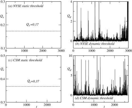
Figure 1: $Q_{s}$ and $Q_{d}(t)$ for the NYSE and CSM are shown in (a), (b), (c) and (d).

where $T$ is the total time interval, and $N$ is the total stock number. Since $Q_{s}$ is the average cross-correlation over the total time and all stocks, the static threshold is reasonable in the sense of providing a uniform standard for cross-correlations of all stocks. As shown in figure 1(a) and (c), $Q_{s}$ takes rather small values, 0.17 for the NYSE and 0.37 for the CSM. However, the cross-correlation $G_{ij}(t)$ is defined by the individual price returns, and fluctuate according to the price dynamics. The static threshold may suffer from the large fluctuation of the cross-correlation $G_{ij}(t)$. Hence, we introduce a dynamic threshold $\zeta\sim Q_{d}(t)$,

$$Q_{d}(t)=\frac{2}{N(N-1)}\sum_{i=1}^{N}\sum_{j=i+1}^{N}G_{ij}(t),$$ (5)

$Q_{d}(t)$ takes only the average over all stocks in a single time step, and therefore fluctuates synchronously with the cross-correlations $G_{ij}(t)$. As shown in figure 1(b) and (d), large values of $Q_{d}(t)$ are observed for both the NYSE and the CSM, in addition to the small values for most time steps. Therefore, the dynamic threshold may suppress the large fluctuation induced by $G_{ij}(t)$, and accordingly creates a stable network structure. In this paper, we consider the static threshold from $\zeta=0.25Q_{s}$ to $4Q_{s}$, and the dynamic threshold from $\zeta=0.25Q_{d}$ to $6Q_{d}$.

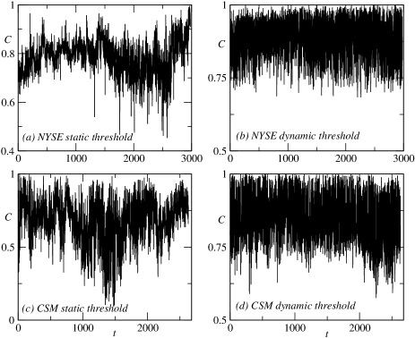
Figure 2: The average clustering coefficients $C(t)$ corresponding to $Q_{s}$ and $Q_{d}(t)$ for the NYSE and CSM are displayed in (a), (b), (c) and (d). The time-averaging values of $C(t)$ are $0.78$, $0.88$, $0.68$ and $0.85$ respectively.

In figure 2, the average clustering coefficient $C(t)$ is displayed for $\zeta=Q_{s}$ and $\zeta=Q_{d}(t)$. The average clustering coefficient $C(t)$ is defined as

$$C(t)=\frac{1}{N}\sum_{i=1}^{N}c_{i}(t),$$ (6)

where $c_{i}(t)$ is the clustering coefficient of node $i$ [24], denoting the ratio of the triangle-connection number of node $i$ to the maximum possible triangle-connection number of the node. It is observed in figure 2 that the average clustering coefficient $C(t)$ of $\zeta=Q_{d}(t)$ is apparently more stable than that of $\zeta=Q_{s}$ for both the NYSE and the CSM. The common characteristic shared by $\zeta=Q_{s}$ and $\zeta=Q_{d}(t)$ is that their average clustering coefficients are large. Especially for the dynamic threshold $\zeta=Q_{d}(t)$, the average clustering coefficient $C(t)$ keeps its values around 0.88 and 0.85 respectively for the NYSE and the CSM at a highly clustering level, implying a close relationship of stocks in the financial markets.

3 Topology dynamics

Topological properties of a complex network are usually described by the average clustering coefficient, the average degree and the cross-correlation of degrees. We investigate the topology dynamics by computing the time-correlations. The autocorrelation function is widely adopted to measure the time-correlation. However, it shows large fluctuations for nonstationary time series. Therefore, we apply the DFA method [34, 35].

For a time series $A(t^{\prime})$, we eliminate the average trend from the time series by introducing $B(t^{\prime})=\sum\limits_{t^{\prime\prime}=1}^{t^{\prime}}[A(t^{\prime\prime})-A_{ave}]$, where $A_{ave}$ is the average of $A(t^{\prime})$ in the total time interval $[1,T]$. Uniformly dividing $[1,T]$ into windows of size $t$, and fitting $B(t^{\prime})$ to a linear function $B_{t}(t^{\prime})$ in each window, we define the DFA function as

$$F(t)=\sqrt{\frac{1}{T}\sum\limits_{t^{\prime}=1}^{T}{[B(t^{\prime})-B_{t}(t^{\prime})]}^{2}},$$ (7)

In general, $F(t)$ will obey a power-law scaling behavior $F(t)\sim t^{\theta}$. The exponent $\theta>1.0$, $0.5<\theta<1.0$ and $0<\theta<0.5$ indicate an unstable, long-range correlating and anti-correlating time series, respectively. $\theta=0.5$ corresponds to the Gaussian white noise, while $\theta=1.0$ represents the $1/f$ noise.

3.1 Average clustering coefficient

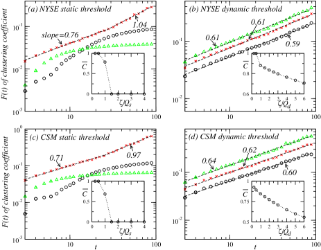
Figure 3: The DFA function of the average clustering coefficient $C(t)$ is plotted on a log-log scale. The inner panel shows the time-averaging clustering coefficient for different threshold values. Dashed lines are the power-law fits. (a) and (c) are of the static thresholds for the NYSE and the CSM. Circles, crosses and triangles are for $\zeta=0.5Q_{s}$, $Q_{s}$ and 2$Q_{s}$, respectively. (b) and (d) are of the dynamic thresholds for the NYSE and the CSM. Circles, crosses and triangles are for $\zeta=Q_{d}(t)$, 2$Q_{d}(t)$ and 3$Q_{d}(t)$, respectively.

The DFA function of the average clustering coefficient $C(t)$ is shown in figure 3. For the static threshold $\zeta=Q_{s}$, a two-stage scaling behavior is observed with a crossover phenomenon in between. For the NYSE, the exponent $\theta$ takes the values $\theta=0.76$ for $t<t_{c}$ and $\theta=1.04$ for $t>t_{c}$. For the CSM, $\theta=0.71$ for $t<t_{c}$ and $\theta=0.97$ for $t>t_{c}$. The crossover time $t_{c}\sim 25$ days. This result indicates that the average clustering coefficients are temporally correlated for $t<t_{c}$, then transit to the $1/f$ noise for $t>t_{c}$. In contrast to that of $\zeta=Q_{s}$, the DFA function of $\zeta=Q_{d}(t)$ shows a clean power-law behavior, with the exponent $\theta=0.59$ for the NYSE and $0.60$ for the CSM, indicating the long-range time correlation.

To investigate the robustness of the above results, and the stability of the network structure during the dynamic evolution, we may adjust the level of the thresholds. For the static threshold, we consider two alternatives $\zeta=0.5Q_{s}$ and $\zeta=2Q_{s}$. As shown in figure 3(a) and (c), one does not find any power-law behavior. In other words, the network structure is rather sensitive to the specific value of the static threshold. For the dynamic threshold, we observe that the DFA function of $C(t)$ remains qualitatively the same for $\zeta\geq Q_{d}(t)$. In figure 3 (b) and (d), for example, the results of $\zeta=2Q_{d}$ and $3Q_{d}$ are displayed. A clean power-law behavior is detected with the exponent $\theta=0.61$ and $0.61$ for the NYSE, and $\theta=0.62$ and $0.64$ for the CSM. Higher dynamic thresholds yield stronger time correlations (i.e., larger values of $\theta$). This implies that the edges created by large $G_{ij}(t)$ are rather stable.

To further understand the topological pattern, we calculate the time-averaging clustering coefficient $\overline{C}$ for different thresholds,

$$\overline{C}=\frac{1}{T}\sum_{t=1}^{T}C(t),$$ (8)

As shown in the inner panel of figure 3(a) and (c), $\overline{C}$ of the static threshold $\zeta\leq 0.5Q_{s}$ is close to 1, but as the threshold increases to 1.5$Q_{s}$, $\overline{C}$ sharply drops to 0. As shown in the inner panel of figure 3(b) and (d), the time-averaging clustering coefficient $\overline{C}$ shows a mild decay for the dynamic threshold, and presents still rather high clustering even for the threshold $\zeta=6Q_{d}(t)$ for both the NYSE and the CSM.

3.2 Average degree

The average degree $K(t)$ of the network is defined as

$$K(t)=\frac{1}{N}\sum_{i=1}^{N}k_{i}(t),$$ (9)

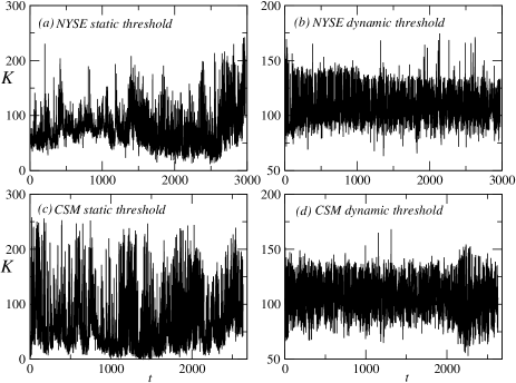
Figure 4: The average degree $K(t)$ is displayed. (a) and (c) are of the static threshold $\zeta=Q_{s}$ for the NYSE and the CSM. (b) and (d) are of the dynamic threshold $\zeta=Q_{d}(t)$ for the NYSE and the CSM.

where $k_{i}(t)$ is the degree of node $i$, denoting the number of the nodes directly connected with it. For $\zeta=Q_{s}$, $K(t)$ exhibits large fluctuations between $0$ and $N-1$, as shown in figure 4(a) and (c). ${K(t)}=N-1$ indicates that every node directly connects to all other nodes in the network, while ${K(t)}=0$ corresponds a set of isolated nodes. The fluctuation of the CSM is obviously stronger, and $K(t)$ often comes rather close to $0$ and $N-1$. For $\zeta=Q_{d}(t)$, $K(t)$ is almost bounded by two envelope curves, as shown in figure 4(b) and (d). The upper envelope is around $K(t)\sim 130$ to $140$, indicating that one node is directly connected to about one half of the nodes on average, while the lower envelope is around $K(t)\sim 70$ to $80$, indicating that one node is directly connected to about one quarter of the nodes on average. The upper envelope implies a high-low symmetric distribution of the cross-correlations $G_{ij}(t)$, with one half of the data points below the average and the other half of the data points above the average. The upper envelope sounds reasonable, for the larger $G_{ij}(t)$ are usually well above the average. However, the lower envelope suggests a high-low asymmetric distribution of the cross-correlations $G_{ij}(t)$. Why there is such a lower envelope remains to be understood.

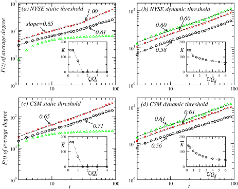
Figure 5: The DFA function of the average degree $K(t)$ is plotted on a log-log scale. Inner panels show the time-averaging degrees for different threshold values. Dashed lines are the power-law fits. (a) and (c) are of the static thresholds for the NYSE and the CSM. Circles, crosses and triangles are for $\zeta=0.5Q_{s}$, $Q_{s}$ and 2$Q_{s}$, respectively. (b) and (d) are of the dynamic thresholds for the NYSE and the CSM. Circles, crosses and triangles are for $\zeta=Q{{}_{d}}(t)$, 2$Q{{}_{d}}(t)$ and 3$Q_{d}(t)$, respectively.

We then compute the DFA function of the average degree $K(t)$. Similar as that of the average clustering coefficient, unstable behavior is detected for the static threshold, whereas stable network structure is observed for the dynamic threshold, as shown in figure 5. For the static threshold, the DFA function for the NYSE shows a power-law behavior with the exponent $\theta=0.61$ for $\zeta=0.5Q_{s}$, a two-stage scaling for $\zeta=Q_{s}$, and no power-law behavior for $\zeta=2Q_{s}$. The DFA function for the CSM shows a power-law behavior with the exponent $\theta=0.65$ and 0.71 for $\zeta=0.5Q_{s}$ and $Q_{s}$, and no power-law behavior for $\zeta=2Q_{s}$. These results can also be understood from the time-averaging degree

$$\overline{K}=\frac{1}{T}\sum_{t=1}^{T}K(t),$$ (10)

As shown in the inner panel of figure 5(a) and (c), the network has a large number of edges for lower static thresholds, however, the number of edges sharply falls off to nearly zero as the threshold increases up to 1.5$Q_{s}$.

For the dynamic threshold, a robust power-law behavior is observed. The exponent $\theta$ of $\zeta=Q_{d}(t)$ is measured to be 0.58 for the NYSE and 0.56 for the CSM respectively, somewhat close to $\theta=1/2$ of the Gaussian white noises. But as $\zeta$ increase, the network structure stabilizes, with the exponent $\theta=0.60$ for the NYSE and 0.61 for the CSM. The time-averaging degree $\overline{K}$ is also found to decay slowly as the dynamic threshold increases, and the network shows significant connections for a high threshold as 6$Q_{d}(t)$, as shown in the inner panel of figure 5(b) and (d).

Why is the dynamic threshold crucial in the analysis of the network structure of financial markets? One important reason is that the volatilities fluctuate strongly in the dynamic evolution. It induces large temporal fluctuations of the cross-correlations of price returns, as is characterized by $Q_{d}(t)$ in figure 1. Thus the static threshold leads to dramatic changes in the topological structure of the network. However, the dynamic threshold proportional to $Q_{d}(t)$ suppresses such a kind of fluctuations, and results in a stable topological structure of the network. For example, we have calculated the time-averaging degree in two typical periods of time for the CSM, i.e., $t=1550$ to $1650$ with small volatilities and $t=2530$ to $2630$ with large volatilities. For the static threshold $\zeta=Q_{s}$, the time-averaging degree is $39$ and $98$ respectively, far away from the time-averaging degree $\overline{K}=68$ in the total time interval. For the dynamic threshold $\zeta=Q_{d}(t)$, however, it is $107$ and $104$ respectively, both around $\overline{K}=107$. Similar results are obtained for the NYSE, and also for the clustering coefficient $C(t)$.

3.3 Degree distribution

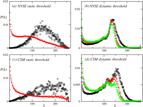
Figure 6: The degree distribution $P(k)$ is displayed on a log-log scale. (a) and (c) are of the static thresholds for the NYSE and the CSM. Circles and crosses are for $\zeta=0.5Q{{}_{s}}$ and $Q{{}_{s}}$ respectively. (b) and (d) are of the dynamic thresholds for the NYSE and the CSM. Circles, crosses and triangles are for $\zeta=Q{{}_{d}}(t)$, 2$Q{{}_{d}}(t)$ and 3$Q_{d}(t)$, respectively.

The degree distribution function $P(k)$ describes the heterogeneous properties of nodes. To obtain a better statistics, we take the degrees of all time steps as an ensemble. Figure 6 shows the degree distribution of the static and dynamic thresholds for the NYSE and the CSM. For both thresholds, it is observed that the degree distribution is different not only from the Poisson distribution, but also from the power-law distribution of a scale-free network. For the static threshold, the degree distribution is rather sensitive to the threshold value, and the form of the degree distribution changes dramatically. For the dynamic threshold, a two-peak behavior is observed with one peak around $k=0$ and the other peak around $k=140\sim 150$ for both the NYSE and CSM. The peak at $k=0$ simply tells that there are a large number of isolated nodes in the network. The peak at $k=140\sim 150$ indicates that one node is directly connected to about one half of the nodes in the network, i.e., the cross-correlation distribution is hight-low symmetric for the dynamic threshold.

The two-peak structure of the degree distribution for the dynamic threshold explains the upper envelope of the average degree $K(t)$ in figure 4. Moreover, the features of the degree distribution is rather robust for different dynamic threshold values. It indicates that the large cross-correlations are much bigger than the average cross-correlation, so that certain increase of $\zeta$ does not alter the network topology.

3.4 Cross-correlation of degrees

The so-called assortative or disassortative mixing on the degrees refers to the cross-correlation of degrees [36, 37]. The ”assortative mixing” means that high-degree nodes tend to directly connect with high-degree nodes, while the ”disassortative mixing” indicates that high-degree nodes prefer to directly connect with low-degree nodes. The cross-correlation of degrees is defined as

$$r(t)=\frac{M^{-1}\sum_{\alpha}{j_{\alpha}k_{\alpha}}-[M^{-1}\sum_{\alpha}{\frac{1}{2}(j_{\alpha}+k_{\alpha})}]^{2}}{M^{-1}\sum_{\alpha}{\frac{1}{2}(j_{\alpha}^{2}+k_{\alpha}^{2})}-[M^{-1}\sum_{\alpha}{\frac{1}{2}(j_{\alpha}+k_{\alpha})}]^{2}},$$ (11)

where $j_{\alpha}$, $k_{\alpha}$ are the degrees of the nodes at both ends of the $\alpha_{th}$ edge, with $\alpha$=1,…,$M$. At a certain time, $r>0$, $r=0$ and $r<0$ represent the assortative mixing, no assortative mixing and disassortative mixing, respectively.

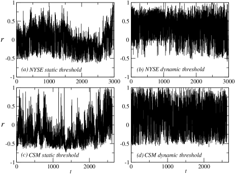
Figure 7: The cross-correlation $r(t)$ of degrees is displayed. (a) and (c) are of the static threshold $\zeta=Q_{s}$ for the NYSE and the CSM. (b) and (d) are of the dynamic threshold $\zeta=Q_{d}(t)$ for the NYSE and the CSM. The time-averaging values of $r(t)$ are $0.00$, $0.36$, $-0.20$ and $0.22$ respectively in (a), (b), (c) and (d).

In figure 7, $r(t)$ of $\zeta=Q_{s}$ and $Q_{d}(t)$ is shown for the NYSE and the CSM. $r(t)$ fluctuates between the interval $[-1,1]$, flipping between the assortative mixing and disassortative mixing during the time evolution. Defining the time-averaging cross-correlation of the degrees,

$$\overline{r}=\frac{1}{T}\sum_{t=1}^{T}r(t),$$ (12)

we obtain $\overline{r}=0.00$ and $-0.20$ of the static threshold for the NYSE and the CSM, $\overline{r}=0.36$ and $0.22$ of the dynamic threshold for the NYSE and the CSM. In other words, the cross-correlation of the static threshold shows no assortative mixing or the disassortative mixing, while that of the dynamic threshold exhibits the assortative mixing.

To study the memory effect, we again compute the DFA function of $r(t)$. As shown in figure 8, the DFA function of $\zeta=Q_{s}$ shows a power-law behavior with the exponent $\theta=0.73$ for the NYSE and 0.77 for the CSM. For $\zeta=0.5Q_{s}$, no power-law behavior is observed. It further confirms the unstable network structure for the static threshold. For the dynamic threshold, the DFA function of $r(t)$ shows nearly a same power-law behavior for $\zeta=Q_{d}(t)$, 2$Q_{d}(t)$ and 3$Q_{d}(t)$, with the exponent $\theta=0.60$ for the NYSE and 0.63 for the CSM.

The community or sector structure identifies different interconnected subsets of networks [13, 14, 15, 38, 39]. To further understand the topological structure of the financial networks, we may investigate the dynamic effect of economic sectors. The random matrix theory is a representative approach to such a problem, e.g., one may analyze the eigenvalues and eigenvectors of the cross-correlation matrix of price returns [13, 14, 15]. With a similar procedure, we first introduce the normalized individual degrees $\widetilde{k}_{i}(t)=(k_{i}-<k_{i}>)/\sigma_{k_{i}}$, with $\sigma_{k_{i}}$ being the standard deviation of $k_{i}$. We then construct the cross-correlation matrix $\mathbf{F}$ of individual degrees $\widetilde{k}_{i}(t)$, whose elements

$$F_{ij}=\frac{1}{T}\sum^{T}_{t=1}\widetilde{k}_{i}(t)\widetilde{k}_{j}(t),$$ (13)

and compute its eigenvalues and eigenvectors. For the network of the NYSE, we do observe that the largest eigenvalue $\lambda_{0}$ corresponds to the market mode, while other large eigenvalues $\lambda_{i}$ typically represent different economic sectors, as shown in figure 9. For the dynamic threshold, the results are robust when $\zeta$ changes from $Q_{d}(t)$ to $6Q_{d}(t)$. For the static threshold, however, reasonable results are obtained only around $\zeta=Q_{s}$. For the CSM, the dynamic effect of the standard economic sectors is weak, and we need a careful analysis to reveal its unusual sectors as reported in Refs. [14].

4 Conclusion

We investigate the topology dynamics of a financial network by a comparative study with static and dynamic thresholds, based on the daily data of the American and Chinese stock markets. For both stock markets, the dynamic threshold properly suppresses the large fluctuation induced by the cross-correlations of individual stock prices, and creates a rather robust and stable network structure during the dynamic evolution, in comparison to the static threshold. Long-range time-correlations are revealed for the average clustering coefficient, the average degree and the cross-correlation of degrees.

The average clustering coefficient and average degree for both static and dynamic thresholds are large, indicating the strong interactions between stocks in financial markets. A two-peak behavior is observed in the degree distribution for the dynamic threshold, very different from the power-law behavior of a scale-free network.

References

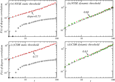
Figure 8: The DFA function of the cross-correlation of degrees is plotted on a log-log scale. Dashed lines are the power-law fits. (a) and (c) are of the static thresholds for the NYSE and the CSM. Circles and triangles are for $\zeta=0.5Q_{s}$ and $Q_{s}$ respectively. (b) and (d) are of the dynamic thresholds for the NYSE and the CSM. Circles, crosses and triangles are for $\zeta=Q{{}_{d}}(t)$, 2$Q{{}_{d}}(t)$ and 3$Q_{d}(t)$, respectively.

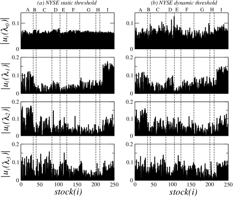
Figure 9: The absolute values of the components $u_{i}$ of stock $i$ for the first four largest eigenvalues of the cross-correlation matrix $\mathbf{F}$ are displayed for the NYSE. Stocks are arranged according to economic sectors separated by dashed lines. A: Basic Materials; B: Conglomerates; C: Consumer Goods; D: Finance; E: Healthcare; F: Industrial Goods; G: Services; H: Technology; I: Utilities. (a) is of the static threshold $\zeta=Q_{s}$, and (b) is of the dynamic threshold $\zeta=Q{{}_{d}}(t)$.

References

- [1] Mantegna R N and Stanley H E 1995 Nature 376 46
- [2] Gopikrishnan P, Plerou V, Amaral L A N and Stanley H E 1999 Phys. Rev. E 60 5305
- [3] Lux T and Marchesi M 1999 Nature 397 498
- [4] Giardina I, Bouchaud J P and Mézard M 2001 Physica A 299 28
- [5] Ren F, Zheng B, Qiu T and Trimper S 2006 Phys. Rev. E 74 041111
- [6] Qiu T, Zheng B, Ren F and Trimper S 2006 Phys. Rev. E 73 065103(R)
- [7] Shen J and Zheng B 2009 Europhys. Lett. 88 28003
- [8] Mantegna R N 1999 Eur. Phys. J. B 11 193
- [9] Bonanno G, Caldarelli G, Lillo F and Mantegna R N 2003 Phys. Rev. E 68 046130
- [10] Micciche S, Bonanno G, Lillo F and Mantegna R N 2003 Physica A 324 66
- [11] Tumminello M, Aste T, Di Matteo T and Mantegna R N 2005 Proc. Natl. Acad. Sci. USA 102 10421
- [12] Tumminello M, Di Matteo T, Aste T and Mantegna R N 2007 Eur. Phys. J. B 55 209
- [13] Plerou V, Gopikrishnan P, Rosenow B, Amaral L A N, Guhr T and Stanley H E 2002 Phys. Rev. E 65 066126
- [14] Shen J and Zheng B 2009 Europhys. Lett. 86 48005
- [15] Coronnello C, Tumminello M, Lillo F, Micciche S and Mantegna R N 2005 Acta Phys. Pol. B 36 2653
- [16] Pan R K and Sinha S 2007 Phys. Rev. E 76 046116
- [17] Utsugi A, Ino K and Oshikawa M 2004 Phys. Rev. E 70 026110
- [18] Garas A, Argyrakis P and Havlin S 2008 Eur. Phys. J. B 63 265
- [19] Albert R, Jeong H and Barabási A L 1999 Nature 401 130
- [20] Albert R and Barabási A L 2002 Rev. Mod. Phys. 74 47
- [21] Caldarelli G, Marchetti R and Pietronero L 2000 Europhys. Lett. 52 386
- [22] Pastor-Satorras R, Vázquez A and Vespignani A 2001 Phys. Rev. Lett. 87 258701
- [23] Barabási A L and Albert R 1999 Science 286 509
- [24] Watts D J and Strogatz S H 1998 Nature 393 440
- [25] May R M and Lloyd A L 2001 Phys. Rev. E 64 066112
- [26] Zhu C P, Zhou T, Yang H J, Xiong S J, Gu Z M, Shi D N, He D R and Wang B H 2008 New J. Phys. 10 023006
- [27] Gross T and Blasius B 2008 J. R. Soc. Interface 5 259
- [28] Onnela J P, Kaski K and Kertész J 2004 Eur. Phys. J. B 38 353
- [29] Huang W Q, Zhuang X T and Yao S 2009 Physica A 388 2956
- [30] Kim H J, Kim I M, Lee Y and Kahng B 2002 J. Korean Phys. Soc. 40 1105
- [31] Song D M, Jiang Z Q and Zhou W X 2009 Physica A 388 2450
- [32] Yang Y and Yang H J 2008 Physica A 387 1381
- [33] Kim K, Kim S Y and Ha D H 2007 Comput. Phys. Commun. 177 184
- [34] Peng C K, Buldyrev S V, Havlin S, Simons M, Stanley H E and Goldberger A L 1994 Phys. Rev. E 49 1685
- [35] Peng C K, Havlin S, Stanley H E and Goldberger A L 1995 Chaos 5 82
- [36] Newman M E J 2002 Phys. Rev. Lett. 89 208701
- [37] Newman M E J and Park J 2003 Phys. Rev. E 68 036122
- [38] Palla G, Derenyi I, Farkas I and Vicsek T 2005 Nature 435 814
- [39] Palla G, Barabási A L and Vicsek T 2007 Nature 446 664