The dark matter halo shape of edge-on disk galaxies

This is the first paper of a series in which we will attempt to put constraints on the flattening of dark halos in disk galaxies. We observe for this purpose the HI in edge-on galaxies, where it is in principle possible to measure the force field in the halo vertically and radially from gas layer flaring and rotation curve decomposition respectively. In this paper, we define a sample of 8 HI rich late-type galaxies suitable for this purpose and present the HI observations.

1 Introduction

Since the 1970’s, it has been known that the curvature of the universe is remarkably flat. This implies that the ratio of the total density to critical density is $\Omega_{tot}\approx 1$. At this time, it was also known from measurements of stars and gas that the mass density of luminous matter is $\Omega_{lum}\lower 2.15277pt\hbox{$\;\buildrel<\over{\sim}\;$}0.005$ — less than $0.5\%$ of that required for a flat $\Omega_{tot}\sim$1 universe. Indeed, the missing matter controversy had begun in the 1930’s when Oort (1932), following Kapteyn (1922), and Zwicky (1937) independently found evidence for vast amounts of unseen matter on different scales. Oort’s analysis of the spatial and velocity distribution of stars in the Solar neighbourhood concluded that luminous stars comprised approximately half the total mass indicated by their motion, assuming gravititational equilibrium. Zwicky’s analysis of the velocity dispersions of rich clusters found that approximately $90-99\%$ of the mass was unseen, if the systems were gravitationally bound. Later on, the inventory of the mass in the Solar neighbourhood showed that the dark matter in the galactic disk at the solar galactocentric radius was mostly fainter stars and interstellar gas (e.g. Holmberg & Flynn, 2000). Zwicky’s value of the velocity dispersion in the Coma cluster is close to the current one (e.g. Colless & Dunn, 1996), and, despite the presence of hot X-ray emitting gas, there must be dark matter to cause $\Omega_{matter}\sim 0.2-0.3$.

Table 1: HI observations

Galaxy	Other	Date	Telescope	Array	Project	Observer	Integration
	name				ID		time (hr)
ESO074-G015	IC5052	11-12 FEB 2001	ATCA	375	C934	Ryan	1.67
ESO074-G015	IC5052	13-14 APR 2001	ATCA	750D	C934	Ryan	2.21
ESO074-G015	IC5052	24-25 FEB 2002	ATCA	1.5A	C894	O’Brien	10.23
ESO074-G015	IC5052	01 DEC 2002	ATCA	6.0A	C894	O’Brien	10.63
ESO074-G015	IC5052	17 OCT 1992	ATCA	6.0C	C212	Carignan	10.05
ESO109-G021	IC5249	20-22 MAR 2003	ATCA	EW352	CX043	Dahlem	8.54
ESO109-G021	IC5249	03-04 FEB 2003	ATCA	750D	C894	O’Brien	8.01
ESO109-G021	IC5249	28 NOV 2002	ATCA	6.0A	C894	O’Brien	13.43
ESO109-G021	IC5249	18 OCT 1992	ATCA	6.0C	C212	Carignan	11.11
ESO115-G021		09 FEB 2005	ATCA	EW352	C1341	Koribalski	10.09
ESO115-G021		06 JAN 2005	ATCA	750B	C1012	Hoegaarden	11.17
ESO115-G021		23 JUN 1995	ATCA	750B	C073	Walsh	7.57
ESO115-G021		08 SEP 2002	ATCA	6.0C	C894	O’Brien	6.51
ESO115-G021		03 DEC 2002	ATCA	6.0A	C894	O’Brien	10.05
ESO115-G021		13 DEC 2002	ATCA	6.0A	C894	O’Brien	5.72
ESO138-G014		08-09 NOV 2002	ATCA	1.5A	C894	O’Brien	10.43
ESO138-G014		29-30 NOV 2002	ATCA	6.0A	C894	O’Brien	9.79
ESO146-G014		17 JAN 2002	ATCA	750A	C894	O’Brien	1.37
ESO146-G014		27-29 DEC 2000	ATCA	750C	C894	O’Brien	10.70
ESO146-G014		11 JAN 2001	ATCA	750C	C894	O’Brien	1.67
ESO146-G014		31 JUL 2001	ATCA	1.5A	C894	O’Brien	7.78
ESO146-G014		14-15 APR 2002	ATCA	6.0A	C894	O’Brien	10.19
ESO146-G014		27-28 JAN 2002	ATCA	6.0B	C894	O’Brien	10.51
ESO274-G001		29 AUG 1993	ATCA	1.5B	C073	Walsh	6.07
ESO274-G001		07 OCT 1993	ATCA	1.5D	C073	Walsh	6.80
ESO274-G001		28-29 NOV 2002	ATCA	6.0A	C894	O’Brien	9.63
ESO435-G025	IC2531	12 JAN 2002	ATCA	750A	C894	O’Brien	9.63
ESO435-G025	IC2531	17 JAN 2002	ATCA	750A	C894	O’Brien	2.02
ESO435-G025	IC2531	07 MAR 1997	ATCA	1.5D	C529	Bureau	9.07
ESO435-G025	IC2531	06 APR 1996	ATCA	6.0A	C529	Bureau	9.94
ESO435-G025	IC2531	13-14 SEP 1996	ATCA	6.0B	C529	Bureau	9.96
ESO435-G025	IC2531	17-18 OCT 1992	ATCA	6.0C	C212	Carignan	7.45
UGC07321		26,30 MAY 2000	VLA	C	AM649	Matthews	16.00
UGC07321		01 NOV 2000	ATCA	1.5D	C894	O’Brien	2.49

Modern dark matter research began in 1970 with several papers which found that galaxies contain more gravitating matter than can be accounted for by the stars. Freeman (1970) noted that the atomic hydrogen (HI) rotation curves of the late-type disk galaxies NGC300 and M33 peaked at a larger radius than expected from the stellar light distribution. This implied that the dark matter was more extended than the stellar distribution and that its mass was at least as great as the luminous mass. However, these data were of poor angular resolution. At the same time Rubin & Ford (1970) published a rotation curve of M31 based on optical data, which did not seem to decline in the outer parts. In the 1970s radio observations of increasingly better angular resolution and better sensitivity showed that flat rotation curves are typical in spiral galaxies (Shostak, 1971; Rogstad & Shostak, 1972; Roberts & Rots, 1973; Bosma, 1978) and that the HI extent of a spiral galaxy can be far greater than the extent of the optical image. This, combined with surface photometry, leads to very high mass-to-light ratios in the outer parts, as shown clearly for several galaxies in Bosma (1978) and Bosma & van der Kruit (1979).

In 1974, dark matter halos were found to extend even further, when Ostriker et al. (1974) and Einasto et al. (1974) tabulated galaxy masses as a function of radius and found that galaxy mass increased linearly out to at least $100$ kpc and $10^{12}$ M_⊙ for normal spirals and ellipticals. Despite this large dark matter fraction inferred in galaxies, it was still not sufficient to reach the critical $\Omega_{tot}\sim$1 value of a flat universe. See e.g. Sofue & Rubin (2001) and Roberts (2008) for a brief history of dark matter in galaxies.

Around the same time, application of nuclear physics to Big Bang theory showed that big bang nucleosynthesis (BBNS) in the early universe produced specific abundances of the light elements, and predicted the total baryon density was $\Omega_{b}\approx 0.044$. In the last decade, the combined observations of high redshift SNIa, (Reiss et al., 1998; Perlmutter et al., 1999), the 2-Degree Field Galaxy Redshift Survey (2dFGRS) (Percival et al., 2001) and WMAP microwave background measurements (Spergel et al., 2003) confirmed the baryonic mass density $\Omega_{b}$ found by BBNS and established that dark energy comprises about $75\%$ of the critical density. Consequently, the scale of the missing dark matter is now reduced. The mass density $\Omega_{m}$ is now only $0.25$, but the problem remains: the measured baryonic mass density is still only $\sim$18% of the total mass density $\Omega_{m}$. Thus, dark matter accounts for $82\%$ of mass in the universe, and baryonic matter is only 4.5% of the total content of the universe.

More than 1000 galactic rotation curves have now been measured, and very few display a Keplerian decline with radius. HI and H$\alpha$ rotation curves of spiral galaxies show that the total-mass-to-light ratios are typically M/L = 10-20 M_⊙/L_⊙, and the luminous matter therefore accounts for only $5-10\%$ of the total mass inferred from the rotation curves. For low surface brightness (LSB) disk galaxies (de Blok, 1997) and dwarf irregular (dI) galaxies (Swaters, 1999), the M/L values increase to 10-100 M_⊙/L_⊙, with an extreme of $220$ for ESO215-G009, a gas-rich LSB galaxy with a very high gas mass to light ratio of $M_{\rm HI}/L_{B}=21$ and low recent star formation (Warren et al., 2004).

Dwarf spheroidal (dSph) galaxies, with typical total masses of only $\sim$10⁷ M_⊙ within radii of a few hundred parsecs, are even more extreme: several have very large dark matter fractions with mass-to-light ratios in the range $200-1000$ M_⊙/L_⊙. In these faint, small galaxies, the dynamical mass is estimated from the line-of-sight velocities of individual stars. The Ursa Major dSph (Willman et al., 2005), is one of the most dark matter dominated galaxies known to date with a central mass-to-light ratio $M/L\sim$500 M_⊙/L_⊙, which is believed to increase further at larger radii (Kleyna et al., 2005). These systems appear to have only very small baryonic mass fractions.

The rotation curves of disk galaxies are important probes of the equatorial halo potential gradient. By decomposing the observed rotation curve into contributions from the visible mass components, the radial potential gradient of the halo can be measured, assuming the system is in centrifugal equilibrium. The dark halo mass component is typically fitted by a pseudo-isothermal halo model with density

$$\rho(R)=\rho_{0}\left[1+\left(\frac{R}{R_{c}}\right)^{2}\right]^{-1},$$ (1)

where the halo is characterised by its central density $\rho_{0}$ and core radius $R_{c}$. Pseudo-isothermal halos have an asymptotic density $\rho\propto R^{-2}$ at large radii which is consistent with commonly flat rotation curves.

Kormendy & Freeman (2004) compiled the published dark halo density distributions for a large sample of Sc-Im and dSph galaxies, and found well-defined scaling relationships for the dark halo parameters for galaxies spanning a range of 6 decades of luminosity. They found that halos of less luminous and massive dwarf spheroidals have higher central densities, up to $\sim$1 M_⊙ pc^-3 and core radii of $\sim$0.1 kpc, compared to $\sim 10^{-3}$ M_⊙ pc^-3 and $\sim$30-100 kpc respectively, for large bright Sc galaxies. The observed correlations suggest a continuous physical sequence of dark halo population in which the properties of the underlying dark halo scale with the baryon luminosity (Kormendy & Freeman, 2004).

We now consider the flattening of the dark halo density distribution, defined by $q=c/a$, where $c$ is the halo polar axis and $a$ is the major axis in the galactic plane. The vertical distribution of the halo is much more difficult to measure than the radial distribution in the equatorial plane, as most luminous tracers of the galaxy potential gradient lie in the plane of the galaxy and offer little indication of the vertical gradient of the potential. Past measurements that were obtained with a variety of different methods gave a large range of $q$ from $0.1$ to $1.37$, with no concentration on any particular value. For our Galaxy, the halo shape has been measured more than ten times by four different methods, that yielded $q-$values ranging from $0.45$ to $1.37$.

In this series of papers, we will use the flaring of the HI gas layer to measure the vertical flattening of the dark halo, because we believe this method to be the most promising for late-type disk galaxies. Like all steady state mass components of a galaxy, the gaseous disk of an isolated disk galaxy can be assumed to be in hydrostatic equilibrium in the gravitational potential of the galaxy, unless there are visible signs from the gas distribution and kinematics that the HI layer is disturbed (e.g. by mergers or local starbursts). In the vertical direction, the gradient of gas pressure is balanced by the gravitation force (ignoring any contribution from a magnetic pressure gradient). From the observed distribution of the gas velocity dispersion and the gas density distribution, we can in principle measure the total vertical gravitational force.

Table 2: Resolution of HI observations

	Spatial		Spectral
Galaxy	resolution		resolution
	(arcsec)	(kpc)	(km s-1)
ESO074-G015	9.0 $\times$ 9.0	0.292 $\times$ 0.292	3.298
ESO109-G021	8.0 $\times$ 8.0	1.179 $\times$ 1.179	3.298
ESO115-G021	8.9 $\times$ 8.9	0.194 $\times$ 0.194	3.298
ESO138-G014	10.7 $\times$ 10.7	0.965 $\times$ 0.965	3.298
ESO146-G014	7.6 $\times$ 7.6	0.793 $\times$ 0.793	3.298
ESO274-G001	9.8 $\times$ 9.8	0.162 $\times$ 0.162	3.298
ESO435-G025	9.0 $\times$ 9.0	1.305 $\times$ 1.305	3.298
UGC07321	15.0 $\times$ 15.0	0.727 $\times$ 0.727	5.152

Euler’s equation for a steady-state fluid of density $\rho$, velocity $\mathbf{v}$ and pressure $p$ in a gravitational potential $\Phi$ is $-\mathbf{(v.\nabla)v}=\rho^{-1}\mathbf{\nabla}p+\mathbf{\nabla}\Phi$. In the case of a vertically Gaussian gas density distribution with a vertically isothermal gas velocity dispersion, the gradient of the total vertical force $K_{z}$ in the $z$-direction can be calculated directly from the gas velocity dispersion $\sigma_{v,g}(R)$ and the gas layer thickness FWHM${}_{z,g}(R)$, each of which are functions of radius:

$$\frac{\partial K_{z}}{\partial z}=-\frac{\sigma_{v,g}^{2}}{({\rm FWHM}_{z,g}/2.35)^{2}}.$$ (2)

It is possible to measure the halo shape over the entire HI extent of the luminous disk using the flaring of the HI distribution, which typically extends in radius to $2-3R_{25}$, and by measuring the density distribution of the gas and stellar distributions. For a given vertical gas velocity dispersion, a more flattened dark halo requires decreased flaring and increased gas surface density. The relatively high gas content of late-type galaxies allows measurement of both the halo vertical force field from the gas layer flaring and the halo radial force field from rotation curve decomposition. In this series of papers we will attempt to measure the halo flattening using the flaring of HI disk in eight small late-type disk galaxies.

Table 3: Noise of HI channel maps

Galaxy	Noise			Max Signal-
	(Jy/beam)	(atoms cm-2)	(K)	to-noise
ESO074-G015	0.00135	1.8348 $10^{19}$	10.0	14.5
ESO109-G021	0.00125	2.1464 $10^{19}$	11.7	10.1
ESO115-G021	0.00113	1.5774 $10^{19}$	8.6	18.6
ESO138-G014	0.00197	1.9008 $10^{19}$	10.4	15.2
ESO146-G014	0.00143	2.7190 $10^{19}$	14.9	11.3
ESO274-G001	0.00151	1.7209 $10^{19}$	9.4	14.6
ESO435-G025	0.00123	1.6789 $10^{19}$	9.2	10.9
UGC07321	0.00038	1.8579 $10^{18}$	1.0	93.0

The main advantage of this method is that it can be used for all gas-rich spiral galaxies inclined sufficiently to measure accurate kinematics, unlike some methods which are applicable only to specific kinds of galaxies like polar ring galaxies. This minimum inclination was determined to be $i\lower 2.15277pt\hbox{$\;\buildrel>\over{\sim}\;$}60^{\circ}$ by Olling (1995). This method was first tried by Celnik et al. (1979) on the Galaxy, and early development was undertaken by van der Kruit (1981), who applied it to low resolution observations of NGC891 and concluded that the halo was not as flattened as the stellar disk. It was then used for several galaxies in the 1990’s, most notably the careful study of the very nearby Sc galaxy NGC4244 which was found to have a highly flattened halo with $q=0.2^{+0.3}_{-0.1}$ out to radii of $\approx 2R_{25}$ (Olling, 1996).

All applications of the HI flaring method to date have derived highly flattened halo distributions ($q\leq 0.5$). With the exclusion of NGC4244, we suspect that the assumption of a radially-constant gas velocity dispersion led to errors in the measured total vertical force, and thereby to the derived flattening of the halo. The other difficulty for all these galaxies except NGC4244 is that they are large galaxies with peak rotation speeds $>170$ km s^-1. Given that (i) spiral galaxies typically have HI velocity dispersions in the relatively small range $6-10$ km s^-1(Tamburro et al., 2009) and (ii) the halo shape $q$ is roughly proportional to the gradient of the vertical force, we see from Eqn. 2 that the HI thickness is to first order inversely proportional to the peak rotation speed. Consequently, the HI flaring method should work best for small disk galaxies with relatively low rotation speeds, as these galaxies should exhibit more HI flaring. Bosma (1994) already showed by calculations that flaring is relatively more important in galaxies with low circular velocity.

The flaring method has also been applied to the Galaxy by Olling & Merrifield (2000). However, uncertainty in the position and rotation speed of the Sun resulted in a large uncertainty of the measured halo shape $0.5\leq q\leq 1.25$.

Table 4: HI measurements

Galaxy	RA	Dec	PA	Dist	$v_{sys}$	$v_{max}$
			(∘)	(Mpc)	(km s-1)	(km s-1)
ESO074-G015	20 52 05.57	–69 12 05.9	141.3	6.70	590.7	93.4
ESO109-G021	22 47 06.07	–64 50 00.6	14.9	30.40	2360.1	112.4
ESO115-G021	02 37 47.28	–61 20 12.1	43.4	4.93	512.2	64.4
ESO138-G014	17 06 59.22	–62 04 58.3	134.4	18.57	1508.4	120.4
ESO146-G014	22 13 00.08	–62 04 05.5	47.3	21.45	1691.1	70.2
ESO274-G001	15 14 13.84	–46 48 28.6	36.9	3.40	522.8	89.4
ESO435-G025	09 59 55.77	–29 37 01.1	74.5	29.89	2477.0	236.3
UGC07321	12 17 34.56	+22 32 26.4	81.8	10.00	401.9	112.1
Galaxy	$W_{20}$	$W_{50}$	FI	$M_{\rm HI}$	Diam.
	(km s-1)	(km s-1)	(Jy km s-1)	(M⊙)	(arcmin)	(kpc)
ESO074-G015	160.8	186.8	37.9	4.0 108	9.350	18.2
ESO109-G021	211.4	224.8	10.9	2.4 109	5.020	44.4
ESO115-G021	112.2	128.9	72.0	3.4 108	13.600	19.5
ESO138-G014	226.3	240.8	51.0	4.2 109	9.210	49.8
ESO146-G014	127.7	140.4	8.4	9.1 108	3.840	24.0
ESO274-G001	167.7	178.8	152.6	4.2 108	16.550	16.4
ESO435-G025	460.9	472.7	13.1	2.8 109	7.300	63.5
UGC07321	209.1	224.2	38.3	9.0 108	9.580	27.9

In this first paper we discuss the selection of our sample and present HI observations. In paper II we will review methods to derive the information we need for our analysis from these data, namely the rotation curves and the HI distributions, HI velocity dispersion and the flaring of the HI layer, all as a function of radius in the deprojected galaxy plane. Paper III will be devoted to applying this to our data and presenting the results for each individual galaxy. In paper IV will analyse the data of one galaxy in our sample, namely UCG7321 and we will set limits on the flattening of its dark halo.

2 Observations

2.1 Sample selection

We selected a sample of southern disk galaxies, for observation with the Australia Telescope Compact Array (ATCA), that were small, HI-rich and late-type, in order to maximise the expected flaring and the likelihood that the HI brightness would be sufficient to probe the low surface densities needed to measure the vertical structure of disk galaxies.

The galaxies were chosen to be edge-on (optical major-to-minor axis ratio $a/b\geq 10$) to simplify HI modelling and increase the accuracy of the measured HI density and kinematics. We avoided galaxies at Galactic latitude $|b|<10^{\circ}$ to reduce Galactic extinction in the optical bands. To minimise uncertainties in the stellar mass distribution we chose relatively bulgeless galaxies with Hubble type Scd-Sd. The galaxies were chosen to be nearer than $30$ Mpc to enable the flaring of the HI to be resolved with the $6$″ ATCA synthesised beam. At $30$ Mpc the FWHM of the ATCA beam is $\sim$1 kpc. The vicinity of each galaxy was searched in NED for nearby neighbours to ensure that it was isolated. The HI masses of all galaxies satisfying these criteria were measured from the HI Parkes All-Sky survey (HIPASS) online data release. With a minimum HI flux integral of $15$ Jy km s^-1, this limited our sample to only 5 galaxies.

The nearest isolated thin edge-on galaxy, ESO274-G001, was added to the sample. Although it had a Galactic latitude of $9.3^{\circ}$, it is exceptionally close at $3.4$ Mpc in the Centaurus A galaxy group, allowing the HI disk to be measured at a resolution of $\sim$150 pc. A search of HI observations in the VLA archive revealed the superthin northern Sd galaxy UGC7321 which we also added to our sample. We also added the Sb galaxy IC2531 to our sample, since it has an extended HI disk and a large quantity of archival observations available. The range of maximum rotation velocity of our sample galaxies in shown in column 7 of Table 4. With the inclusion of IC2531, a galaxy with a box/peanut bulge, and hence barred (Bureau & Freeman, 1999), we attempt to measure the halo shape of galaxies spanning different mass scales and stages of secular evolution.

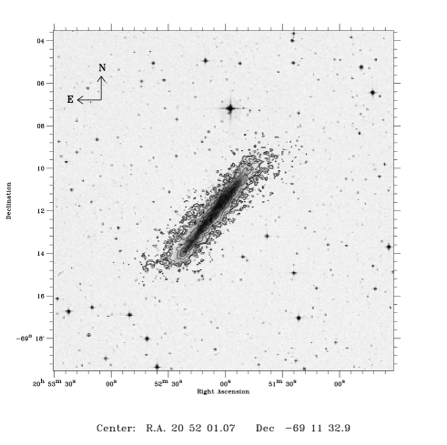
Figure 1: ESO074-G015 (IC5052). HI column density map overlaid on the DSS image. Contours are plotted in $(3,5,10,25,50,80)\times\sigma$, where the rms noise $\sigma=2.05$ mJy beam^-1or $2.79\times 10^{19}$ atoms cm^-2. The FWHM synthesised beam has dimensions $9.0\arcsec\times 9.0\arcsec$, and is displayed as a cross-hatched symbol in the lower left.

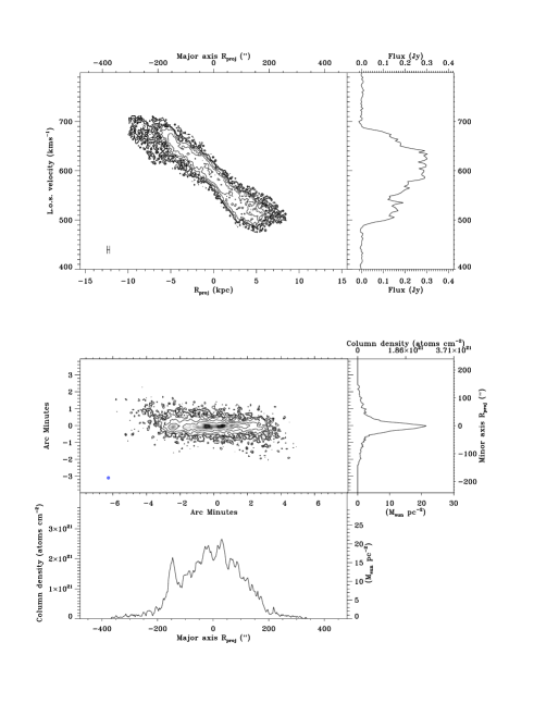
Figure 2: ESO074-G015 (IC5052). Top left: XV map. XV contours are $(3,5,10,25,50,100)\times\sigma$, where the rms noise $\sigma=1.90$ mJy beam^-1or $2.58\times 10^{19}$ atoms cm^-2. The half power beam extent over the major axis is shown in the lower left corner. Top right: Integrated spectrum. Middle left: HI column density map rotated with the galaxy major axis aligned with the X axis. Column density map contours are $(3,5,10,25,50,100)\times\sigma$, where the rms noise $\sigma=1.65$ mJy beam^-1 or $2.24\times 10^{19}$ atoms cm^-2. The synthesised beam has dimensions $9.0\arcsec\times 9.0\arcsec$, and is displayed as a cross-hatched symbol in the lower left. Middle right: Minor axis profile. Bottom left: Major axis profile.

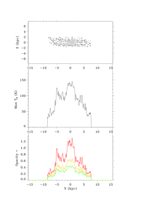
Figure 4: ESO074-G015 (IC5052). Top : Peak brightness temperature map. Contours are plotted in $(35,75,120)\times\sigma$, where the rms noise is $10.0$ K. The FWHM synthesised beam has dimensions $9.0\arcsec\times 9.0\arcsec$. Middle: Major axis peak brightness temperature profile. Bottom: Inferred HI opacity calculated assuming constant HI spin temperatures. The resulting maximum opacities along each line of sight column through the galaxy disk are plotted for $T_{spin}$ = 200, 300 and 400 K (bottom to top).

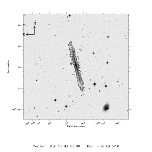
Figure 5: ESO109-G021 (IC5249). HI column density map overlaid on the DSS image. Contours are plotted in $(3,5,10,25,50)\times\sigma$, where the rms noise $\sigma=1.81$ mJy beam^-1or $3.11\times 10^{19}$ atoms cm^-2. The FWHM synthesised beam has dimensions $8.0\arcsec\times 8.0\arcsec$, and is displayed as a cross-hatched symbol in the lower left.

Figure 5: ESO109-G021 (IC5249). Top left: XV map. XV contours are $(3,5,10,20,40)\times\sigma$, where the rms noise $\sigma=1.76$ mJy beam^-1or $3.03\times 10^{19}$ atoms cm^-2. The half power beam extent over the major axis is shown in the lower left corner. Top right: Integrated spectrum. Middle left: HI column density map rotated with the galaxy major axis aligned with the X axis. Column density map contours are $(3,5,10,25,50)\times\sigma$, where the rms noise $\sigma=1.62$ mJy beam^-1or $2.79\times 10^{19}$ atoms cm^-2. The FWHM synthesised beam has dimensions $8.0\arcsec\times 8.0\arcsec$, and is displayed as a cross-hatched symbol in the lower left. Middle right: Minor axis profile. Bottom left: Major axis profile.

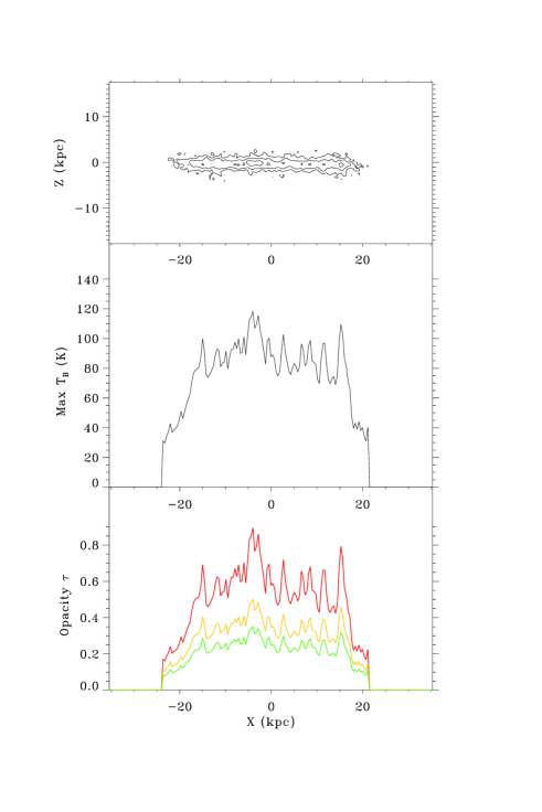
Figure 6: ESO109-G021 (IC5249). Top : Peak brightness temperature map. Contours are plotted in $(35,58,93)\times\sigma$, where the rms noise is $11.7$ K. The FWHM synthesised beam has dimensions $8.0\arcsec\times 8.0\arcsec$. Middle: Major axis peak brightness temperature profile. Bottom: Inferred HI opacity calculated assuming constant HI spin temperatures. The resulting maximum opacities along each line of sight column through the galaxy disk are plotted for $T_{spin}$ = 200, 300 and 400 K (bottom to top).

2.2 Observing modes and method

Galaxies were observed with the ATCA in a range of array configurations to obtain high spatial resolution across each galaxy. In addition, available observations from the ATCA and VLA archives were also used. The list of observations is shown in Table 1. Column 8 shows the integration time in hours of each observation. The resulting resolution and sensitivity of the HI observations are shown in Table 2 and Table 3, respectively. We have smoothed the data in Right Ascension to match that in Declination, providing the smallest circular beam possible. The spatial resolutions shown in Table 2 correspond to the FWHM of the resulting beams.

At the ATCA the XX and YY polarisations were used, with a spectral channel width of $3.3$ km s^-1. At the VLA the RR and LL polarizations were used, and the channel width was $5.2$ km s^-1. Due to the narrow bandwidth available with the VLA correlator at the time of observations, multiple overlapping bandpasses were observed to fully span the velocity width of the target galaxies. For those observations, each bandpass was calibrated and imaged separately, and the resulting subcubes glued together along the spectral axis.

3 Data reduction and imaging

A detailed account and discussion of the data reduction and imaging procedures is given in the online appendix. Here we restrict ourselves to a brief synopsis.

The reduction of the HI data was performed with the radio interferometry data reduction package miriad. The data were calibrated in the usual manner, using primary and secondary flux calibrators. Solar and terrestrial interference peaks in the calibrator scans were inspected, and flagged if necessary. The bandpass calibration was done using either the primary or, in case of sufficient signal-to-noise ratio, the secondary calibrator. After calibration, the target data were inspected for interference, and flagged appropriately. The radio continuum contribution to each channel map was removed in the uv-plane, by using a suitable average of line-free channel maps.

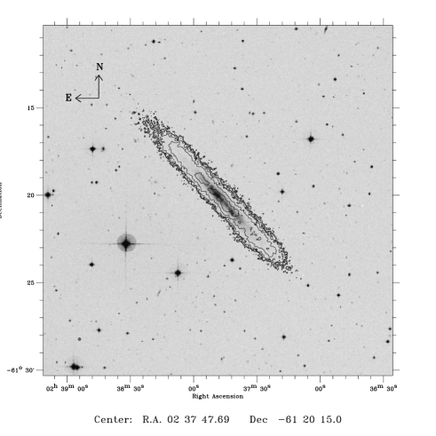
Figure 7: ESO115-G021. HI column density map overlaid on the DSS image. Contours are plotted in $(3,5,10,25,50)\times\sigma$, where the rms noise $\sigma=1.76$ mJy beam^-1or $2.44\times 10^{19}$ atoms cm^-2. The FWHM synthesised beam has dimensions $8.9\arcsec\times 8.9\arcsec$, and is displayed as a cross-hatched symbol in the lower left.

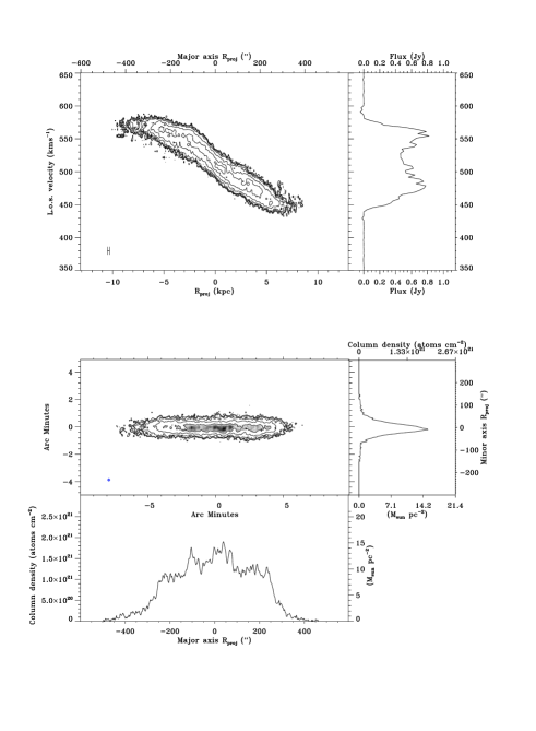
Figure 6: ESO115-G021. Top left: XV map. XV contours are $(3,5,10,20,50,100,150)\times\sigma$, where the rms noise $\sigma=1.55$ mJy beam^-1or $2.16\times 10^{19}$ atoms cm^-2. The half power beam extent over the major axis is shown in the lower left corner. Top right: Integrated spectrum. Middle left: HI column density map rotated with the galaxy major axis aligned with the X axis. Column density map contours are $(3,5,10,25,50)\times\sigma$, where the rms noise $\sigma=1.47$ mJy beam^-1 or $2.04\times 10^{19}$ atoms cm^-2. The FWHM synthesised beam has dimensions $8.9\arcsec\times 8.9\arcsec$, and is displayed as a cross-hatched symbol in the lower left. Middle right: Minor axis profile. Bottom left: Major axis profile.

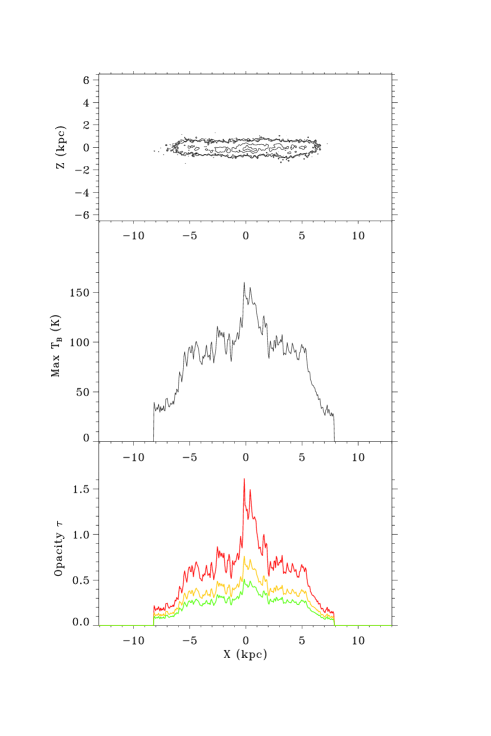
Figure 6: ESO115-G021. Top : Peak brightness temperature map. Contours are plotted in $(35,42,86,129)\times\sigma$, where the rms noise is $8.6$ K. The FWHM synthesised beam has dimensions $8.9\arcsec\times 8.9\arcsec$. Middle: Major axis peak brightness temperature profile. Bottom: Inferred HI opacity calculated assuming constant HI spin temperatures. The resulting maximum opacities along each line of sight column through the galaxy disk are plotted for $T_{spin}$ = 200, 300 and 400 K (bottom to top).

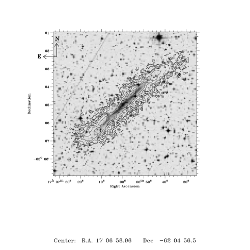
Figure 7: ESO138-G014. HI column density map overlaid on the DSS image. Contours are plotted in $(3,5,10,25,50,100)\times\sigma$, where the rms noise $\sigma=2.84$ mJy beam^-1or $2.73\times 10^{19}$ atoms cm^-2. The FWHM synthesised beam has dimensions $10.7\arcsec\times 10.7\arcsec$, and is displayed as a cross-hatched symbol in the lower left.

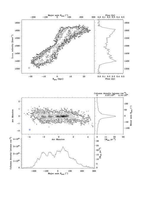
Figure 5: ESO138-G014. Top left: XV map. XV contours are $(3,5,10,20,50)\times\sigma$, where the rms noise $\sigma=2.74$ mJy beam^-1 or $2.64\times 10^{19}$ atoms cm^-2. The half power beam extent over the major axis is shown in the lower left corner. Top right: Integrated spectrum. Middle left: HI column density map rotated with the galaxy major axis aligned with the X axis. Column density map contours are $(3,5,10,25,50,75,100)\times\sigma$, where the rms noise $\sigma=2.38$ mJy beam^-1 or $2.29\times 10^{19}$ atoms cm^-2. The FWHM synthesised beam has dimensions $10.7\arcsec\times 10.7\arcsec$, and is displayed as a cross-hatched symbol in the lower left. Middle right: Minor axis profile. Bottom left: Major axis profile.

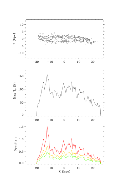
Figure 4: ESO138-G014. Top : Peak brightness temperture map. Countours are plotted in $(41,51,83,124)\times\sigma$, where the rms noise is $10.4$ K. The FWHM synthesised beam has dimensions $10.7\arcsec\times 10.7\arcsec$r. Middle: Major axis peak brightness temperature profile. Bottom: Inferred HI opacity calculated assuming constant HI spin temperatures. The resulting maximum opacities along each line of sight column through the galaxy disk are plotted for $T_{spin}$ = 200, 300 and 400 K (bottom to top).

4 HI emission

4.1 The HI distribution

To make the HI column density map, the intensity of each channel map was first converted from flux density $I(x,y)$ in units of Jy beam^-1 to HI column density $N_{\rm HI}$ in atoms cm^-2 using

$$N_{\rm HI}(v)=\left(\frac{1.101974351\times 10^{24}}{\theta_{maj}\,\theta_{min}}\right)I(x,y),$$ (3)

where $\theta_{maj}$ and $\theta_{min}$ are the major and minor axis FWHM of the synthesised beam in arcsec. The HI column density maps were made by taking the zeroth moment of masked channel maps (with $v$ in km s^-1):

$$N_{\rm HI}=\int N_{\rm HI}(v)dv.$$ (4)

To exclude any residual sidelobes, a loose region mask was defined interactively for each channel map and then all pixels with flux density above a nominal clip level of 2-3$\sigma$ in each masked channel map were integrated. This procedure ignores faint, low-level HI emission and the resulting integrated HI maps will not contain any extended, low surface brightness component in the gas distribution. However, this does not have an effect on the general distribution of HI as determined by our method. The maps in this paper have been produced to show the general distribution of the gas in the disk in order to judge the suitability of the galaxies for further study. We will only be able to analyse the flaring and velocity dispersion as long as we can obtain high signal-to-noise profiles. A search for extended HI is beyond the scope of our present analysis of the data. As the number of channels integrated to form the column density map varies as a function of position, the noise in the HI column density map also varies accordingly. In order to approximate the noise of the HI column density map, a noise map was also constructed. The noise at each position in the map was calculated as

$$\sigma_{total}=\sqrt{n_{\rm ch}}\times\langle\sigma_{\rm ch}(v)\rangle,$$ (5)

where $\langle\sigma_{\rm ch}(v)\rangle$ is the mean rms noise of all channel maps integrated at that position. By dividing the column density map by the noise map a signal-to-noise ratio map was formed. Following the method of Kregel et al. (2004), the rms noise of the column density map was calculated from the average flux density of all pixels with a signal-to-noise ratio between 2.75 and 3.25.

4.2 Global properties

The integrated HI spectrum was measured from the HI data cube using the HI column density map to mask the cube, and integrating over the area of the galaxy mask. This flux density spectrum was converted to units of Jy by dividing by the synthesised beam area

$$S(v)=\frac{1}{1.133\,\theta_{maj}\,\theta_{min}}\int I(x,y)dxdy.$$ (6)

As the flux was integrated over an equal area in each channel map, the noise of each channel is

$$\sigma_{tot}=\sqrt{{\rm Area}_{\rm HI}}\times\sigma_{\rm ch},$$ (7)

where Area_HI is the area of HI column density emission, and $\sigma_{\rm ch}$ is the rms noise of each channel map. For HI cubes with a constant rms noise in each channel, the noise of the spectrum was fitted from the line-free channels in the spectrum. The velocity widths at the $20\%$- and $50\%$-levels ($W_{20}$, $W_{50}$, respectively) were measured from the spectrum, and the spectrum was integrated over the velocity range spanned by $W_{20}$ to get the integrated flux, FI:

$${\rm FI}=\int^{W_{20,high}}_{W_{20,low}}S(v)dv.$$ (8)

The restriction of the integration to the velocity range $W_{20}$ introduces a small but systematic error in the total flux, underestimating it by no more than a few %. However, for our present purposes it is important to examine the integrated profile in order to identify major asymmetries that would make the galaxy unsuitable for our purposes.

The total HI mass, $M_{\rm HI}$ was then measured from the flux integral using the formula

$$M_{\rm HI}=2.35D^{2}\times{\rm FI},$$ (9)

where the adopted distance $D$ is given in Mpc. These HI measurements are shown in Table 4. These total masses are also underestimated by a few %.

The centre of each galaxy was obtained from the HI column density map by rotating the image by $180^{\circ}$ and finding the optimal pixel offset of the rotated image relative to the original image by maximising the correlation function of the two images using the IDL Astronomy User’s Library function correl_optimize. Formally this gives the center of the HI disk rather than the galactic rotational center. Comparison to the coordinates given in the NASA/IPAC Extragalactic Database NED, which are derived from the Two Micron All Sky Survey 2MASS, show differences of on average only 4 arcsec per coordinate, except for ESO074-G015, where it is about 20 arcsec in RA and 30 arcsec in Dec. However, this galaxy shows some deviations from symmetry, both in optical appearance as well as in the HI distribution. The position adopted fits the symmetry of the XV map very well (see Fig. 2) and is also closer to centers listed in NED that are derived from photographic and IRAS data.

The position angle of the galaxy was found by a similar method. First a wide range of position angles were trialed around the estimated position angle. The HI column density map was reflected over each test position angle about the galaxy center and the residual of the two maps was calculated. The position angle that yielded the lowest summed residual was then adopted as the next position angle estimate. Subsequent rounds spanned smaller and smaller ranges of the position angle until the position angle was determined to less than $0.1\deg$ or until the total residual dropped below $1\%$ of the summed flux of the HI column density map. Both methods worked very well for observations with a near circular synthesised beam, achieving an accuracy of $\sim$1 pixel in the centre position and $0.1-0.2\deg$ in position angle. However, observations with a highly elongated beam were poorly fitted, as the distortion of the image caused by the beam shape biased the derived PA towards the PA of the synthesised beam. For such observations the uncertainty of the measured centre and position angle were larger.

The xzv cube was constructed by rotating the HI data cube about the galaxy center to align the galaxy major axis with the X axis. In Sect. 5 we show the rotated channel maps to allow the flaring to be viewed directly from the observations. We also present the HI column density map with the projected major and minor axis profiles as measured from the HI column density map. The HI diameter and maximum vertical extent were measured at the $3\sigma$ level of the projected profiles.

An XV cube was also produced by reordering the cube axes to form a xvz cube. This cube was then integrated over the $z$ axis to make an XV map using the same method as was used to make the HI column density map. Both the XV map and the HI column density map are shown with their respective noise levels in Sect. 5. The systemic velocity of the galaxy was measured from the XV map by shifting the XV distribution flipped in V with respect to the actual XV map to maximise the correlation function.

Peak brightness temperature maps were also made for each galaxy, where the peak brightness temperature is the maximum brightness temperature over all channel maps at each spatial position. The brightness temperature $T_{B}$ was derived from the HI column density $N_{\rm HI}$ in each channel map using

$$T_{B}=\frac{N_{\rm HI}}{1.83\times 10^{18}}.$$ (10)

The major axis profile of the peak brightness map is also shown for each galaxy in Sect. 5. These plots are useful indicators of possible HI self-absorption that could be obscuring the intrinsic HI surface distribution. Sect. 5 also shows the inferred HI opacity of the brightest HI emission at each major axis position, assuming three different values of the HI spin temperature ($200,300,400$ K).

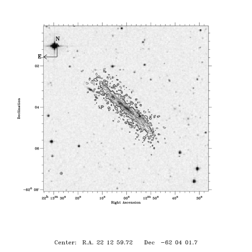
Figure 5: ESO146-G014. HI column density map overlaid on the DSS image. Contours are plotted in $(3,5,10,25,50)\times\sigma$, where the rms noise $\sigma=1.53$ mJy beam^-1 or $2.92\times 10^{19}$ atoms cm^-2. The FWHM synthesised beam has dimensions $7.6\arcsec\times 7.6\arcsec$, and is displayed as a cross-hatched symbol in the lower left.

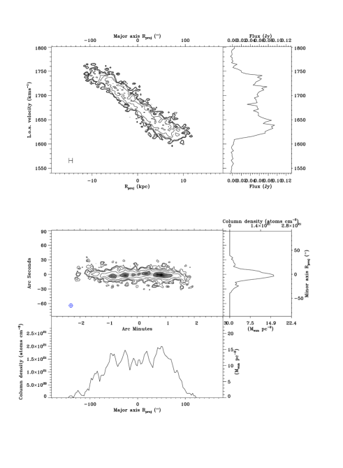
Figure 2: ESO146-G014. Top left: XV map. XV contours are $(3,5,10,25,50)\times\sigma$, where the rms noise $\sigma=1.45$ mJy beam^-1 or $2.76\times 10^{19}$ atoms cm^-2. The half power beam extent over the major axis is shown in the lower left corner. Top right: Integrated spectrum. Middle left: HI column density map rotated with the galaxy major axis aligned with the X axis. Column density map contours are $(3,5,10,25,50)\times\sigma$, where the rms noise $\sigma=1.40$ mJy beam^-1 or $2.67\times 10^{19}$ atoms cm^-2. The FWHM synthesised beam has dimensions $7.6\arcsec\times 7.6\arcsec$, and is displayed as a cross-hatched symbol in the lower left. Middle right: Minor axis profile. Bottom left: Major axis profile.

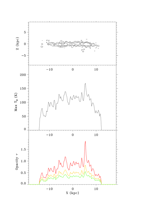
Figure 0: ESO146-G014. Top : Peak brightness temperature map. Contours are plotted in $(60,80,100)\times\sigma$, where the rms noise is $14.9$ K. The FWHM synthesised beam has dimensions $7.6\arcsec\times 7.6\arcsec$. Middle: Major axis peak brightness temperature profile. Bottom: Inferred HI opacity calculated assuming constant HI spin temperatures. The resulting maximum opacities along each line of sight column through the galaxy disk are plotted for $T_{spin}$ = 200, 300 and 400 K (bottom to top).

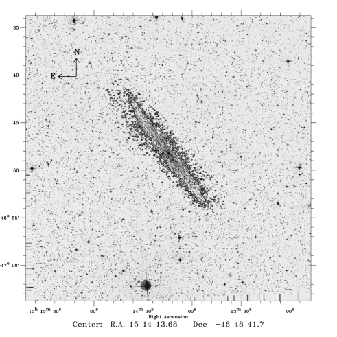
Figure 1: ESO274-G001. HI column density map overlaid on the DSS image. Contours are plotted in $(3,5,10,25,50)\times\sigma$, where the rms noise $\sigma=2.02$ mJy beam^-1 or $2.30\times 10^{19}$ atoms cm^-2. The FWHM synthesised beam has dimensions $9.8\arcsec\times 9.8\arcsec$, and is displayed as a cross-hatched symbol in the lower left.

Figure -3: ESO274-G001. Top left: XV map. XV contours are $(3,5,10,25,50,100)\times\sigma$, where the rms noise $\sigma=2.24$ mJy beam^-1 or $2.56\times 10^{19}$ atoms cm^-2. The half power beam extent over the major axis is shown in the lower left corner. Top right: Integrated spectrum. Middle left: HI column density map rotated with the galaxy major axis aligned with the X axis. Column density map contours are $(3,5,10,25,50,100)\times\sigma$, where the rms noise $\sigma=1.70$ mJy beam^-1 or $1.93\times 10^{19}$ atoms cm^-2. The FWHM synthesised beam has dimensions $9.8\arcsec\times 9.8\arcsec$, and is displayed as a cross-hatched symbol in the lower left. Middle right: Minor axis profile. Bottom left: Major axis profile.

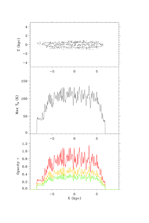
Figure -6: ESO274-G001. Top : Peak brightness temperature map. Contours are plotted in $(40,100)\times\sigma$, where the rms noise is $9.4$ K. The FWHM synthesised beam has dimensions $9.8\arcsec\times 9.8\arcsec$. Middle: Major axis peak brightness temperature profile. Bottom: Inferred HI opacity calculated assuming constant HI spin temperatures. The resulting maximum opacities along each line of sight column through the galaxy disk are plotted for $T_{spin}$ = 200, 300 and 400 K (bottom to top).

5 Results for individual galaxies

In this section we present our data for the galaxies in the sample. For each galaxy we present the following figures. Part a shows an HI column density map overlaid on an optical image from the Digitized Sky Survey (DSS). Part b shows the total intensity position-velocity map (XV map) together with the integrated spectrum, and the HI column density map aligned with the major axis of the galaxy and the corresponding major and minor axis surface density profiles. Part c shows the peak brightness temperature map and the corresponding observed major axis profile and compares this with opacity profiles calculated with some assumed HI spin temperatures. The individual channel maps were presented by O’Brien (2007) and are included in further parts d, e etc. (depending on how many figures are needed) as online-only material at the end of this paper.

5.1 ESO074-G015 (IC5052)

ESO074-G015 is a SBd galaxy with a substantial star formation region extending above and below the galactic plane on the west side of the galactic centre. However despite this, the HI column density distribution (shown in Fig. 2) is surprisingly symmetric. Although there is extensive high latitude HI gas extending to $3.7$ kpc above and $4.2$ kpc below the galactic equator, the distribution of elevated gas appears to be similar on both sides of the galactic centre. Similarly the XV diagram is also fairly symmetric. There is a slight decrease in flux along the line-of-nodes of the west side of the galaxy possibly indicating gas depletion due to a star burst. However there is no apparent localised region of high velocity dispersion gas that could be associated with the star burst.

The HI distribution extends to a maximum radial extent of $281$″ or $9.1$ kpc (for the adopted distance of $6.7$ kpc). The scalelength of the projected distribution $h_{X}$ is $\approx 120$ ″ or $3.9$ kpc, with the edge of the HI disk at $2.3h_{X}$. The exponential scaleheight of the projected minor axis distribution $h_{z}$ is $20.5$ ″ or $667$ pc. The high latitude HI clouds extend to a height of $3.9$ kpc or $6$ scaleheights away from the equatorial plane.

The galaxy is well-resolved by the synthesised beam along the major axis, extending to $31$ FWHM beamwidths on each side of the galactic centre, where each FWHM beamwidth is $292$ pc. In the vertical direction the measured scaleheight of the projected distribution is approximately $4\times$ HWHM beamwidth, indicating that the vertical HI structure is well-resolved by the synthesised beam. Indeed the high latitude HI gas extends to $13\times$ HWHM beamwidth. Vertical flaring of the gas distribution can be noted in the extreme velocity channels $499,509,657,667,677$ km s^-1  in the outer part of the galaxy where the rotation curve inferred from the XV map is roughly flat.

The HI column density distribution is dominated by two bright spots at a projected radius of $\sim$1 kpc from the centre. The brightest gas emission in the cube with brightness temperatures of approximately $140$ K also correspond to this position. The HI disk also contains two outer bright points (although less defined on the western side) at a radius of $\sim$5-6 kpc with a equatorial brightness distribution similar to that of the barred galaxy UGC7321, which also displays the characteristic “figure-8” pattern of a bar in its XV distribution. Although ESO074-G015 is classified as a barred SBd galaxy in NED, it does not display a “figure-8” pattern in the XV map. ESO074-G015 contains only $1/3$ of the HI mass of UGC7321, and has a lower maximum rotation speed of $90.1$ km s^-1, relative to $112.1$ km s^-1 for UGC7321. It is possible that the lower angular momentum and overall mass of ESO074-G015 restricts gas flow in the orbital patterns of a barred potential.

5.2 ESO109-G021 (IC5249)

ESO109-G021 is a superthin Sd galaxy with B-band stellar scalelength-to-scaleheight ratio of $11$ (van der Kruit et al., 2001). The rotation curve was initially found to be in solid body rotation by Abe et al. (1999), however van der Kruit et al. (2001) pointed out such a rotation curve was inconsistent with the double-horned HI spectrum (see Fig. 5). By modelling the XV diagram van der Kruit et al. (2001) show that ESO109-G21 is differentially rotating.

To improve signal-to-noise and recovery of image structure we obtained two additional $12$-hour synthesis observations at the ATCA and added these to the earlier observation by Carignan which was used in the rotation curve analysis by Abe et al. (1999) and van der Kruit et al. (2001). The distance of ESO109-G21 is about $30$ Mpc distant so the HI beam is relatively large, $1179$ pc. The HI column density map in Fig. 5 shows the galaxy to be well-resolved in the radial direction, while perpendicular to the plane the resolution is just sufficient to detect flaring in the extreme velocity channel maps. Comparison of the XV map in Fig. 5 with that measured by van der Kruit et al. (2001) shows significantly improved structure recovery. However the peak signal-to-noise of the HI channel maps is $10.1$, which will make measurement of the HI flaring quite difficult.

5.3 ESO115-G021

This Scd galaxy extends to a maximum radial extent of $445$″ or $9.7$ kpc (assuming a Hubble flow distance of $4.5$ kpc inferred from the $v_{Gal}$). The scalelength of the projected distribution, $h_{X}$, is $209$″ or $4.6$ kpc, with the edge of the HI disk at $2.1h_{X}$. This HI column density map (Fig. 6) displays a very symmetric disk which appears to be relatively quiescent with no obvious HI extensions above and below the inner disk. The vertical structure is well-resolved, extending to a height of $1.7$ kpc, equivalent to 8.5 FWHM beamwidths or $2.9h_{z}$, where $h_{z}$ is the projected scaleheight of $26.7$ arcsec or $583$ pc . The flaring of the vertical HI distribution can clearly be seen in channel maps at $459,469,479,548,558,568$ km s^-1, particularily on the eastern side where the flatter domain of the rotation curve is more extended (as inferred from the XV map shown in Fig. 6).

The XV diagram does not display barred gas kinematics; however a small galaxy like ESO115-G021 with a rotation speed of $62$ km s^-1 is unlikely to show the strong orbital patterns of a gas bar. The HI column density distribution is dominated by a plateau within a radius of $5$ kpc, except for a central bright peak with a peak brightness of $\sim$150 K in the central $1$ kpc.

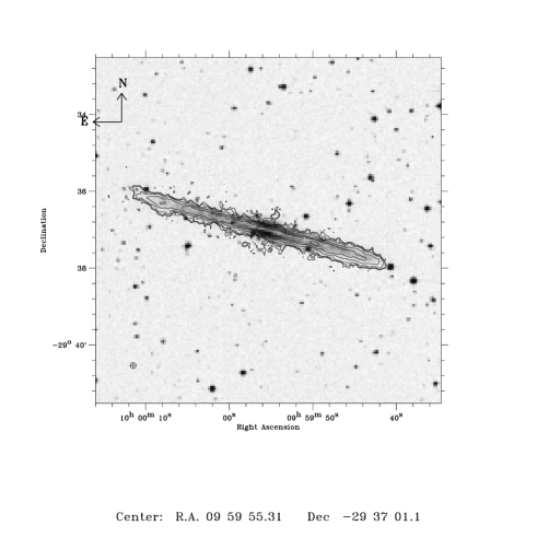
Figure -5: ESO435-G025 (IC2531). HI column density map overlaid on the DSS image. Contours are plotted in $(3,5,10,25,50,100)\times\sigma$, where the rms noise $\sigma=1.73$ mJy beam^-1or $2.35\times 10^{19}$ atoms cm^-2. The FWHM synthesised beam has dimensions $9.0\arcsec\times 9.0\arcsec$, and is displayed as a cross-hatched symbol in the lower left.

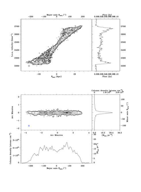
Figure -10: ESO435-G025 (IC2531). Top left: XV map. XV contours are $(3,5,10,20,30)\times\sigma$, where the rms noise $\sigma=1.76$ mJy beam^-1 or $2.40\times 10^{19}$ atoms cm^-2. The half power beam extent over the major axis is shown in the lower left corner. Top right: Integrated spectrum. Middle left: HI column density map rotated with the galaxy major axis aligned with the X axis. Column density map contours are $(3,5,10,25,50,100)\times\sigma$, where the rms noise $\sigma=1.68$ mJy beam^-1 or $2.28\times 10^{19}$ atoms cm^-2. The FWHM synthesised beam has dimensions $9.0\arcsec\times 9.0\arcsec$, and is displayed as a cross-hatched symbol in the lower left. Middle right: Minor axis profile. Bottom left: Major axis profile.

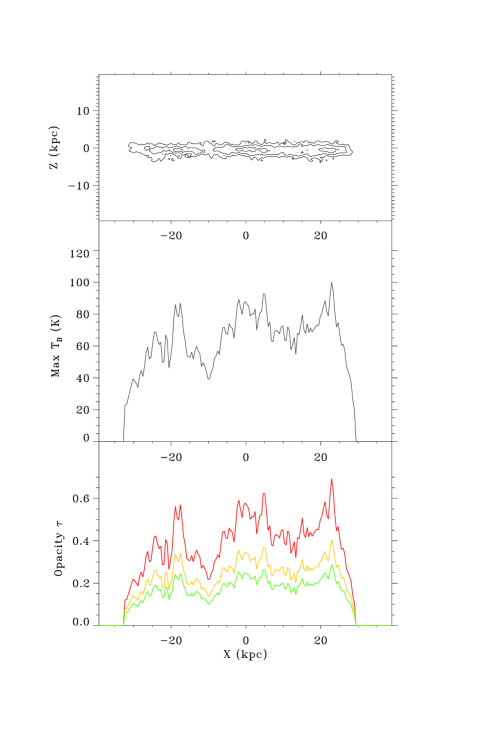
Figure -14: ESO435-G025 (IC2531). Top : Peak brightness temperature map. Contours are plotted in $(27,46,73)\times\sigma$, where the rms noise is $9.2$ K. The FWHM synthesised beam has dimensions $9.0\arcsec\times 9.0\arcsec$. Middle: Major axis peak brightness temperature profile. Bottom: Inferred HI opacity calculated assuming constant HI spin temperatures. The resulting maximum opacities along each line of sight column through the galaxy disk are plotted for $T_{spin}$ = 200, 300 and 400 K (bottom to top).

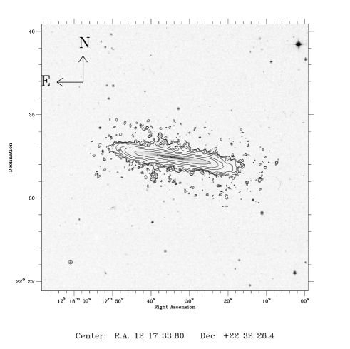
Figure -13: UGC7321. HI column density map overlaid on the DSS image. Contours are plotted in $(3,5,10,25,50,100,250,500)\times\sigma$, where the rms noise $\sigma=$ 0.524 mJy beam^-1 or 2.57$\times 10^{18}$ atoms cm^-2. The FWHM synthesised beam has dimensions $15.0\arcsec\times 15.0\arcsec$, and is displayed as a cross-hatched symbol in the lower left.

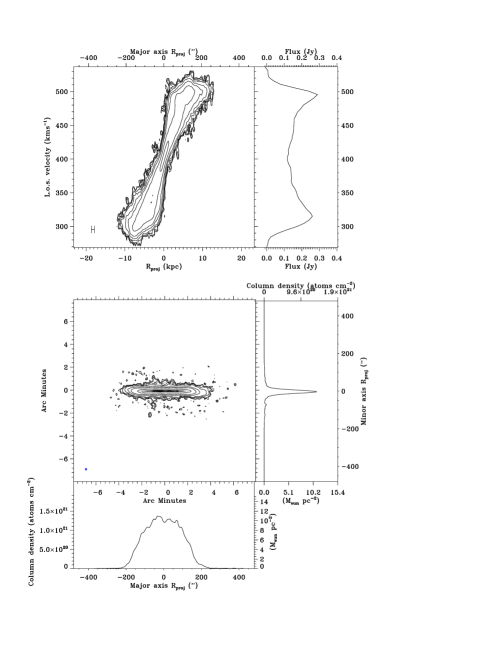
Figure -19: UGC7321. Top left: XV map. XV contours are $(3,5,10,20,50,100,250,500)\times\sigma$, where the rms noise $\sigma=0.524$ mJy beam^-1 or $2.57\times 10^{18}$ atoms cm^-2. The half power beam extent over the major axis is shown in the lower left corner. Top right: Integrated spectrum. Middle left: HI column density map rotated with the galaxy major axis aligned with the X axis. Column density map contours are $(3,5,10,20,50,100,250,500)\times\sigma$, where the rms noise $\sigma=0.508$ mJy beam^-1 or $2.49\times 10^{18}$ atoms cm^-2. The FWHM synthesised beam has dimensions $15\arcsec\times 15\arcsec$, and is displayed as a cross-hatched symbol in the lower left. Middle right: Minor axis profile. Bottom left: Major axis profile.

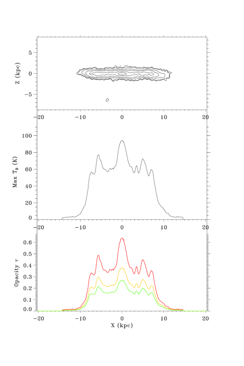
Figure -24: UGC7321. Top : Peak brightness temperature map. Contours are plotted in $(4,5,10,20,50,80)\times\sigma$, where the rms noise is $1.0$ K. The FWHM synthesised beam has dimensions $15\arcsec\times 15\arcsec$. Middle: Major axis peak brightness temperature profile. Bottom: Inferred HI opacity calculated assuming constant HI spin temperatures of $200$, $300$ and $400$ K. The resulting maximum opacities along each line of sight column through the galaxy disk are plotted for $T_{spin}$ = 200, 300, and 400 K (bottom to top).

5.4 ESO138-G014

ESO138-G14 is a larger Sd galaxy, with a maximum rotation speed of $120.4$ km s^-1 and a HI disk extending to $23$ kpc. The HI column density map in Fig. 7 shows the HI disk is well-resolved by the HI synthesised beam of $10.7$″ or $960$ pc. The XV diagram in Fig. 5 shows depressions in the HI flux at radii of $\sim$10 kpc, with the indication of a “figure-8” structure in the gas kinematics. This suggests that the galaxy is actually barred, as “figure-8” structures are typically seen in gas kinematics of barred edge-on systems (Bureau & Freeman, 1999).

We were able to observe this galaxy only in the 1.5A and 6A ATCA array configurations. Due to the lack of short spacing observations we are missing much of the extended structure on large spatial scales. The channel maps show that the HI disk clearly flares vertically with radius, but the missing extended structure will hamper accurate measurement of the flaring.

5.5 ESO146-G014

This Sd galaxy extends to a maximum radial extent of $118$″ or $12.3$ kpc (assuming the distance of $21.5$ kpc determined from its systemic velocity). The galaxy is well-resolved by the synthesised beam along the major axis, extending to $15$ FWHM beamwidths on each side of the galactic centre, where each FWHM beamwidth is $793$ pc. In the vertical direction the measured scaleheight of the projected distribution is $2.6$ times the HWHM beamwidth, indicating that the galaxy is well-resolved in the vertical direction also.

ESO146-G014 has a rotation speed of $70.2$ km s^-1, typical of low-mass Sd galaxies. The rotation of ESO146-G014 appears solid body from the XV diagram in Fig. 2, however HI modelling (see Paper III) shows a differential inner rotation curve like other small disk galaxies when observed at high resolution (e.g. Swaters, 1999). The XV diagram shows no evidence of a HI bar, which is as expected given the low oxygen abundance of $6\%$ of the solar value (Bergvall & Ronnback, 1995).

5.6 ESO274-G001

ESO274-G001 is the closest galaxy in our sample, at a distance of $3.4$ Mpc in the Centaurus A group. Its proximity allows the HI disk to be examined at $160$ pc resolution with the $9.8$″ resolution of the HI synthesised beam. To image this galaxy we used two partial observations in 1.5 km ATCA array configurations from the ATCA archive, and one new 12-hour synthesis observation in the ATCA 6A array configuration. From the HI total column density map in Fig. 1 we can see that the vertical axis is very well-resolved, although it is clear from the diffuse structure that the significant extended HI emission is not observed due to the lack of observations in short array configurations. Comparison of the HI flux integral with that measured from the HI Parkes All-Sky Survey (HIPASS) data shows that about 30% of the HI flux is not measured.

From the XV map in Fig. -3 we see that the rotation curve of this small Sd galaxy rises steeply to a radius of $1-2$ kpc and then flattens on one side, but continues to rise with a shallower slope on the other side. In these outer velocity channel maps, where the HI spans a larger range along major axis, it is possible to see clear flaring of the gas thickness with radius. However, the galaxy is lopsided kinematically, and also slightly lopsided in its HI distribution with an indication of a warp on the NE side.

5.7 ESO435-G025 (IC2531)

ESO435-G25 is the only large spiral galaxy in our sample. It is an Sb galaxy with a bright peanut-shaped bulge shown to be a bar from the “figure-8” signature in the optical emission line kinematics (Bureau & Freeman, 1999). The line splitting faintly seen as a figure-8 signature in the HI XV diagram in Fig. -10 was first detected by Bureau & Freeman (1997). We use the same ATCA HI observations in our study.

The HI column density map shows the galaxy extends to $\sim$25 beamwidths on either side of the galactic centre, and three beamwidths on either side of the HI midplane. Above the galactic centre, the HI column density map in Fig. -5 shows HI filaments extending to $\sim$3 kpc above and below the midplane. Like ESO109-G021, the other distant galaxy, the peak signal-to-noise is quite low at $10.9$. Although the HI disk appears to be flared in the HI column density map (Fig. -5), the flaring is not visibly obvious in the HI channel maps due to the low signal-to-noise.

5.8 UGC7321

This Sd galaxy extends to a maximum radial extent of $288$″ or $14.0$ kpc (assuming the distance of $10$ kpc adopted by Uson & Matthews (2003)). The scalelength of the projected distribution, $h_{X}$, is $112$″ or $5.4$ kpc, with the edge of the HI disk at $2.6h_{X}$. This galaxy exhibits substantial high latitude HI extending up to $144$″ or $7.0$ kpc in the inner HI disk. The scaleheight of the projected minor axis distribution $h_{z}$ is $11.6$ ″ or $560$ pc. Thus the high latitude HI clouds extend to a height of $12$ scaleheights above the equatorial plane.

The galaxy is well-resolved by the synthesis beam along the major axis, extending to $19$ FWHM beamwidths on each side of the galactic centre, where each FWHM beamwidth is $727$ pc. In the vertical direction the measured scaleheight of the projected distribution is similar to the FWHM beamwidth, suggesting that the low latitude vertical structure is dominated by the shape of the synthesised beam. However despite the relatively large synthesised beam, the vertical flaring is clearly visible in most channel maps due to the extended roughly flat rotation curve which is clearly apparent in the XV map (Fig. -19).

The XV diagram (Fig. -19) also exhibits the characteristic “figure-8” shape, which can be indicative of barred HI dynamics (Kuijken & Merrifield, 1995; Bureau & Freeman, 1999; Athanassoula & Bureau, 1999; Athanassoula, 2000). Further evidence for a dynamical bar in UGC7321 was later found by Pohlen who detected the distinctive boxy-bulge shape in the near-IR distribution (Pohlen et al., 2003). Pohlen et al. (2003) measure the bar length as $112\pm 21$″ or $5.4\pm 1.0$ kpc. This is in agreement with the bar size inferred from the size of the “figure-8” kinematics. It also corresponds to the scalelength of the projected HI profile. The HI column density has a plateau at radii within $5$ kpc, declining steeply at radii outside this radius.

The peak brightness temperature rises steeply at radii inside $2$ kpc to $94$ K. Assuming a HI spin temperature of $200$ or $400$ K, the corresponding central HI opacity $\tau$ is $0.65$ or $0.27$. The two outer peak brightness points correspond to radii of $6$ kpc east, and $5.5$ kpc west, also aligning with the outer Lindblad resonance points of the stellar bar measured by Pohlen et al. (2003).

6 Discussion & Summary

The resolution of our HI data along the major axis is high, with the number of independent beamwidths on each side of the galaxy centre ranging from $15$ to over $50$ in our galaxies. In the vertical direction all galaxies are spanned by at least $5$ beamwidths. Unfortunately three of the galaxies in the sample suffer from incomplete imaging, resulting in missing information about the extended spatial structure due to the lack of observations along short baselines. For two of these galaxies ESO074-G015 and ESO274-G001, the images still contain substantial information due to the small linear size of the beam, $290$ pc and $160$ pc, respectively. For these galaxies the iterative HI modelling methods used to measure the deprojected HI density distribution and kinematics (Paper II) should provide good measurements of the flaring. But the HI images of ESO138-G014 indicate missing extended HI emission and low spatial resolution which will probably prevent reliable measurement of the flaring in this galaxy. All the other galaxies in our sample are promising candidates for accurate measurement of the HI kinematics and vertical flaring.

The HI column density distribution of the galaxies in our sample varies quite substantially. The four galaxies with maximum rotation speeds $\lower 2.15277pt\hbox{$\;\buildrel>\over{\sim}\;$}100$ km s^-1 all have HI disks that extend to greater than $5$ kpc away from the plane. Three of them (ESO435-G25, UGC7321 and ESO138-G14) also have the “figure-8” signature in the XV diagram suggestive of an edge-on bar in the gas distribution. ESO435-G25 (Bureau & Freeman, 1999) and UGC7321 (Pohlen et al., 2003) both have boxy-peanut shaped stellar bulges consistent with a bar seen edge-on. Combined with the figure-8 signature in the HI gas structure this is strong evidence for a bar (Kuijken & Merrifield, 1995; Bureau & Freeman, 1999; Athanassoula & Bureau, 1999; Athanassoula, 2000). E138-G014, IC5249 and IC2531 all have large HI disks with radii larger than $20$ kpc, while UGC7321 is much smaller with a radius of only $14.0$ kpc.

The other four galaxies are not much smaller than UGC7321 in radial extent, but they are considerably smaller in total mass. They also lack the vertical extensions in the central disk that suggest additional sources of heat in the disk. This suggests that one of the causes of extended high latitude HI filaments is heating related to star formation and other processes associated with the bar.

The peak brightness profiles of each galaxy show that the inferred HI opacity (assuming a constant HI spin temperature) varies substantially across the major axis of each galaxy. The high spatial resolution of our images has made it possible to measure high HI brightness temperatures. The maximum brightness temperature in our galaxies ranges from $94.4$ K for UGC7321 to $168.6$ K for ESO146-G14. In addition to ESO146-G14, two other galaxies have high HI brightness temperatures $>150$ K. Assuming a mean HI spin temperature of $300$ K, the maximum inferred opacity for these HI bright galaxies is $\sim$0.7. This is comparable to the maximum HI opacity of $0.85$ measured in NGC891 (Kregel et al., 2004). Inspection of the peak brightness as a function of major axis position for these three galaxies shows that, in each case, the region of increased opacity is localised spanning a projected radius of $\sim$1-2 kpc. In ESO115-G21, this increased opacity region occurs at the galactic centre. However for ESO138-G14 and ESO146-G14, the regions of increased opacity occur in the outer disk. Three of our eight galaxies appear to be warped, and one is lopsided. This is consistent with results from larger samples, as e.g. mentioned in the review by Sancisi et. (2008).

Appendix A Data reduction

A.1 Calibration

Reduction of the HI data was performed with the radio interferometry data reduction package miriad. First, the data was loaded into miriad with the task atlod, using the barycentric velocity reference frame, and specifying the rest frequency of HI. The visibilities were then split into separate datasets for each source. The primary and secondary calibrators for each source were inspected for the characteristic signs of solar and terrestrial radio frequency interference (RFI) using the task uvplt and tvflag. Visibilities with RFI, Galaxy HI emission, shadowing or during known telescope system problems were flagged bad. The primary calibrator data were flux calibrated using the known flux with the task mfcal. The secondary calibrator was then used to calibrate the telescope gains, and if sufficient parallactic angle coverage was obtained with the secondary calibrator it was also used to calibrate the bandpass. For observations with low parallactic angle coverage, such as snapshots, the bandpass solution of the primary calibrator was used to calculate the bandpass.

The calibrated flux solution of both primary and secondary calibrators was inspected with uvplt. New secondary calibrators were calibrated during observations, and then inspected with the task uvflux to see if they resembled an unpolarised point source. If the secondary calibrator was too faint, showed polarisation or structure in L band then it was replaced by the next nearest suitable bright calibrator for later calibrator scans throughout the observing run. Gains and bandpass solutions were inspected with the task gpplt. The flux density of the secondary calibrator was then corrected using the primary calibrator flux solution.

The final calibration tables were copied to the target galaxy visibility dataset. Before applying the calibration, the gains were averaged over the duration of each secondary calibrator pointing (3 minutes) and gains interpolation was limited to the interval between secondary calibrator observations (30-45 minutes).

The calibrated target galaxy visibilities were then inspected with the tasks tvflag, uvplt, and any data contaminated by RFI or shadowing was flagged bad with the appropriate flagging tool (tvflag, uvflag or blflag).

A.2 Continuum subtraction

To identify the presence of radio continuum sources in the field of view, a large $30\arcmin$ channel-averaged (ch0) image was made using the task invert extending out to approximately the half power radius of the primary beam. The positions and flux in radius were fitted for any continuum sources found in the ch0 map using the task cgcurs. The visibility spectra of each baseline were then inspected using the task uvspec. Spectral channels free of HI emission were identified. Observations of nearby galaxies often showed Galactic HI emission within the observed bandpass. It was not necessary to flag these channels. Instead they were excluded from the list of line-free channels used in the continuum subtraction. As the target galaxy HI emission was always separated from the Galaxy line emission by at least $100-200$ km s^-1, they were also not included in the galaxy HI image cubes.

The radio continuum was then removed by performing a low order polynomial fit to the line-free channels with the task uvlin. If the observation included a radio continuum source with flux significantly brighter than the channel-averaged HI flux of the target galaxy, then the phase center was shifted to the position of the brightest contaminating continuum source during the continuum subtraction. The continuum-corrected visibility spectra were checked with the task uvspec and a new large ch0 image was formed to search for additional fainter residual continuum sources that remained after the first continuum subtraction. If found, continuum subtraction was repeated with the phase center shifted to the next brightest source. The process was repeated until the ch0 image showed no significant contaminating continuum sources. For observations that were taken during daylight hours, the continuum subtraction was performed with the phase center shifted to the position of the Sun. This procedure could be compromised by continuum emission from the galaxy itself or background sources and in all cases it worked satisfactorily.

For the narrow bandpass VLA observations, it was not possible to span the full galaxy emission in a single bandpass when using the high spectral resolution correlator configuration. In such cases, the galaxy was imaged with two overlapping bandpasses. As these bandpasses included only a few line-free channels on one side of the bandpass it was not possible to perform an accurate 1st order polynomial fit to the line-free channels with uvlin. Instead any bright continuum sources were subtracted from each bandpass with the task uvmodel using a point source model with the fitted flux and position of the radio source. Any residual continuum emission was removed with a zero-order fit to the few line-free channels in each bandpass. This performed a satisfactory continuum subtraction for the three galaxies observed at the VLA.

Appendix B Imaging

A preliminary dirty HI data cube and dirty beam map was formed using the default gridding where each pixel size is $1/3$ of the synthesised beam FWHM along the X and Y axes of the beam. The accurate beam shape was then measured from the central peak of the dirty beam by fitting an elliptical Gaussian to determine the major $\theta_{maj}$ and minor $\theta_{min}$ axes and position angle of the synthesised beam. The preliminary data cube was used to determine the size and velocity range of the HI emission. A new dirty datacube was then made with square pixels each of $1/3$ or $1/5$ of the synthesised beam FWHM major axis $\theta_{maj}$.

The visibilities were weighted using a robust weighting of 0.4 (Briggs, 1995) to provide a optimal compromise between spatial resolution and suppression of sidelobes. A positive robust weighting causes the visibilities in the more sparsely-sampled parts of the visibility phase space to be down-weighted relative to uniform weighting. This reduces the amplitude of the sidelobes, without significantly increasing the size of the synthesised beam FWHM. The barycentric velocity reference frame and the radio definition of velocity was used for the velocity axis of the HI data cube. We chose the radio definition because it yields a constant velocity increment between channels, which was useful for later modelling of the HI distribution.

We used the miriad clean algorithm to correct for effects introduced by the sparcity of the visibility sampling. To find the approximate HI emission region in a each channel, first an initial clean was performed over the central quarter of each channel map, and a low resolution data cube was made by restoring the clean components with a Gaussian of twice the full resolution synthesised beam size. The noise in each plane of the low resolution cube was then measured, and inspected to find the region of HI emission in each plane. Following standard practise, a clean mask was created by selecting the region in each plane of the low resolution data cube with HI emission greater than twice the rms noise ($2\sigma$) using the task cgcurs. The noise level of the full resolution dirty cube was measured and then the areas defined by the clean mask were cleaned down to $0.5\sigma$ using miriad clean. We realise that this is not the optimal procedure to find the low level emission as CLEAN components found in a high resolution image usually do not represent the low level extended emission properly. Better practice would have been to make low resolution images from the continuum subtracted u,v data directly and CLEAN those. In the case of this study, however, only high resolution images are produced and used.

The final full resolution HI data cube was produced using the task restor which produces a residual map for each channel map by subtracting the transformed clean components, and then adds the restored flux to each residual image by convolving the clean components by the clean beam. A circular Gaussian was used for the clean beam, with the FWHM set by the measured major axis FWHM of the dirty beam. After restoration the full cube was corrected for the effect of the antennae primary beam using the task linmos. The size of the restoring beam is shown in column 2 & 3 of Table 2.

As multiple observations in different array configurations were combined to provide the maximum visibility sampling, resolution and sensitivity, some galaxies were observed at slightly different pointing positions. These observations were imaged using the mosaic mode in invert, and deconvolved using the task mosmem which performs a maximum entropy deconvolution of data with multiple pointings.

In the case of VLA data for which multiple bandpasses were needed to span the galaxy HI emission, the visibility data were split into separate bandpasses prior to imaging, with the overlap region combined using the task uvcat. Each bandpass was then imaged, cleaned and restored separately, before concatenating the final subcubes with the task imcat. Although the channel separation at the joins was not exactly the same as the channel width elsewhere, the difference was less than $1$ km s^-1, which is unlikely to effect subsequent modelling of the HI distribution. The overlap channels were observed for a longer integration time and consequently these channel maps have a lower rms noise. However as channel maps and moment analysis were made using the noise measured in each channel map, the difference in noise level over the velocity range of the galaxy is handled appropriately and does not cause noise contamination in the derived images. The measured noise levels of the HI data cubes are shown in Table 3.

After forming the full resolution HI data cubes with Miriad, all subsequent imaging, moment analysis and measurements were undertaken using the Interactive Data Language (IDL).

Appendix C Channel maps

In (O’Brien, 2007) all the channel maps that contain HI emission have been dispayed as contour diagrams. Interested readers can obtain an electronic .pdf file with these maps upon request from P.C. van der Kruit or K.C. Freeman at the email address given on the first page.