Sublimation of the Martian $\mathrm{CO_{2}}$ Seasonal South Polar Cap

Abstract

The polar condensation/sublimation of $\mathrm{CO_{2}}$, that involve about one fourth of the atmosphere mass, is the major Martian climatic cycle. Early observations in visible and thermal infrared have shown that the sublimation of the Seasonal South Polar Cap (SSPC) is not symmetric around the geographic South Pole.

Here we use observations by OMEGA/Mars Express in the near-infrared to detect unambiguously the presence of $\mathrm{CO_{2}}$ at the surface, and to estimate albedo. Second, we estimate the sublimation of $\mathrm{CO_{2}}$ released in the atmosphere and show that there is a two-step process. From Ls=180° to 220°, the sublimation is nearly symmetric with a slight advantage for the cryptic region. After Ls=220° the anti-cryptic region sublimation is stronger. Those two phases are not balanced such that there is $22\%\pm 9$ more mass the anti-cryptic region, arguing for more snow precipitation. We compare those results with the MOLA height measurements. Finally we discuss implications for the Martian atmosphere about general circulation and gas tracers, e.g. Ar.

1 Introduction

The “cryptic region” is a dark region covered by ice in the South Polar Region of Mars (Kieffer et al. (2000); Titus et al. (2008)). It appears to be a region where most of the “spiders” features are located (Piqueux et al. (2003); Kieffer (2007)). In order to simplify, we define in this article the cryptic region from longitude 50°E to 230°E (through longitude 90°E), and the anti-cryptic region from longitude 130°W to 50°E (the complementary sector, passing through longitude 0°E) (see fig. 1).

During the phase of $\mathrm{CO_{2}}$ frost accumulation, the Seasonal South Polar Cap (SSPC) is mainly formed by direct condensation, but some snow events can occur (Forget et al., 1998). GCM studies show that a topographic forcing by the Hellas basin creates an asymmetry in the mode of deposition. Precipitation events are more frequent for the anti-cryptic sector than for the cryptic sector (Colaprete et al., 2005; Giuranna et al., 2008). This suggests that the texture should be more granular (smaller grain sizes) for the former compared to the latter. This texture difference produces a relatively higher albedo in the anti-cryptic region and also possibly a higher accumulated mass.

The direct measurement of the sublimating $\mathrm{CO_{2}}$ mass on Mars has been done only recently by three different techniques: gravity (Smith et al. (2001); Karatekin et al. (2006)), neutron flux (Litvak et al. (2006)) and gamma ray flux (Kelly et al. (2006)). But the time and space resolutions of these methods prohibit any conclusion at the regional scale. At the present time, only direct measurements of the seasonal variations in altitude by MOLA are able to estimate the local $\mathrm{CO_{2}}$ mass sublimation (Smith et al. (2001); Aharonson et al. (2004); Jian and Ip (2009)). But this impressive technique is limited by low signal to noise ratio because seasonal topographic variations are typically less that one meter! To enhance the climatic signal, Aharonson et al. (2004) use a Fourier transform and apply a filter on the MOLA time variation keeping only the annual period. Results show that the amplitude of this annual Fourier cycle is asymmetric, with a maximum in the anti-cryptic region (see fig. 4 (a) in Aharonson et al. (2004)). This results lead to two different conclusions: (i) asymmetry in amplitude is actually related to asymmetry in accumulation and/or (ii) the annual period filtering may be not relevant to describe the real annual mass variation, so that the amplitude asymmetry may be an artefact related to the time of presence of $\mathrm{CO_{2}}$. The second hypothesis is supported by the fact that the sublimation is much faster in the cryptic region (Kieffer et al. (2000); Langevin et al. (2007)) leading to lower amplitude of the annual Fourier cycle. If this hypothesis is valid, the bi-annual cycle should be stronger for the cryptic region. More recently, Jian and Ip (2009) focus on the south polar region and show that cryptic and non-cryptic regions did not present any significant thickness difference.

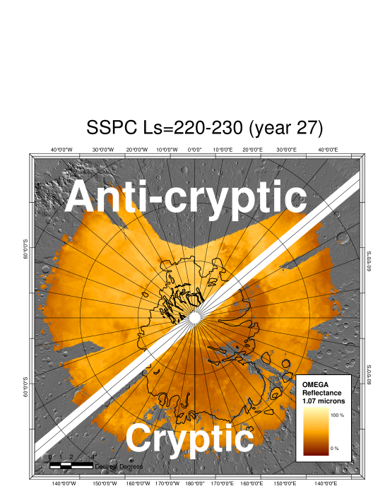
Figure 1: Definition of the cryptic and anti-cryptic region within this article.

Indirect measurement of the $\mathrm{CO_{2}}$ mass has been performed for decades through modeling of: (i) the recession of the surface covered by ice observed by visible/infrared detectors (Leighton and Murray (1966); Paige and Ingersoll (1985); Lindner (1993); Forget (1998); Kieffer et al. (2000); Schmidt et al. (2009c)), (ii) fitting the annual surface pressure cycle (Pollack et al. (1990); Wood and Paige (1992); Hourdin et al. (1995)). The first modeling methodology has the advantage to allow simple estimation of $\mathrm{CO_{2}}$ ice sublimation mass at regional scale. It assumes that the $\mathrm{CO_{2}}$ ice is in vapour-pressure equilibrium with the local atmosphere, and that the $\mathrm{CO_{2}}$ mass balance at the surface is controlled by radiative balance. We propose to use this methodology using the latest OMEGA observation to estimate the local $\mathrm{CO_{2}}$ mass balance in order to derive the difference in the cryptic/anti-cryptic region.

For each considered location on the map, the so-called crocus date is the date (Kieffer et al. (2000)) when the surface deposit is completely gone. The crocus date is then a geophysical field of importance for atmospheric studies. Due to the fact that all instruments have a limited spatial resolution, Schmidt et al. (2009c) has introduced both inner and outer crocus date. Each location is defined by a super pixel with a spatial extent defined by the $L_{stat}$ scale length (with a the pixel scale length $L_{pix}$<$L_{stat}$). The inner crocus date - respectively outer crocus date - is the date when the first - resp. the last - pixels fails to exhibit any ice signature within the considered super pixel (see fig. 2).

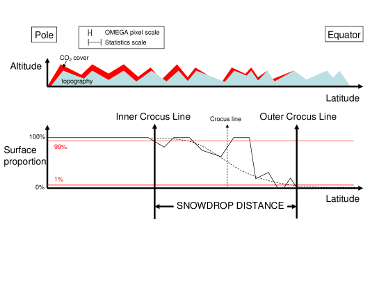
Figure 2: Definition of inner crocus line, outer crocus line and snowdrop distance. Statistics scale length $L_{stat}$ define the super pixel resolution, binning several OMEGA pixels. Black line represents the actual surface proportion covered by $\mathrm{CO_{2}}$ ice for each super pixel. Doted lines represents the arctan model law (Kieffer et al. (2000)). Crocus line is defined in the inflection point of the arctan law. Inner and Outer crocus lines are defined by the surface proportion of 99% and 1%.

We will use the D-frost model (Schmidt et al. (2009c, 2008)) to estimates the $\mathrm{CO_{2}}$ frost mass balance. Several inputs are required: inner and outer crocus dates, albedo, altitude, slope. This model is able to calculate the total mass sublimated, from the date it becomes unstable (determined by the model itself), to the crocus date (determined by the observation). Thus the initial mass, before net sublimation, is not required as an input but will be determined by the model.

The aim of this work is to:

• estimate the main input fields, required for the D-frost model, from OMEGA observations: albedo, inner crocus/outer crocus date.

• calculate the sublimated mass of the SSPC using D-frost.

• derive the height variations, assuming a constant density, and compare to MOLA measurements.

• estimate the spatial asymmetry of the $\mathrm{CO_{2}}$ mass release.

• derive potential effects on circulation at global scale, and on atmospheric gas tracers.

To avoid confusion about the sign of the “sublimation rate” of the SSPC, we adopt two natural conventions: surface convention with negative mass rates (sublimation of seasonal frosts); atmosphere convention, with positive mass rates (pump up of the atmosphere).

2 Methods

We propose to use the OMEGA imaging spectrometer (Bibring et al. (2004)) on board Mars Express for simultaneously detect $\mathrm{CO_{2}}$ ice on Mars and estimate the albedo under the aerosols layer. A compilation of all dataset available is out of the scope of this article but should be an interesting step for the future.

We use the following notation: latitude $\lambda$ , longitude $\theta$ and time $t$. The spatial fields (inner and outer crocus dates) are sampled in a spatial grid of 0.3° latitude (200 steps from $\lambda=-90\text{\textdegree}$ to -30°) and 10° longitude (36 steps from $\theta=0\text{\textdegree}$ to 360°). The spatio-temporal fields (albedo and sublimated mass) are sampled in the same spatial grid and the temporal grid of 5°Ls (72 steps from $t=0\text{\textdegree}$ to 360°). Each element of the grid is called “bin”. The succession of bins in latitude at constant longitude is called a “longitude sector”. Respectively a succession of bins in longitude at constant latitude is called a “latitude sector”

Due to the lack of the spatial/temporal cover we need to interpolate the measured crocus dates and albedo. The first two sections present our strategy. Each of these interpolation methods will be evaluated simply using the standard deviation of the difference between the actual data and the interpolated field.

2.1 Crocus dates field

For each bin with available OMEGA observation, we estimate the inner and outer crocus dates using previously described method in Schmidt et al. (2009c). This method uses WAVANGLET, an automatic detection algorithm (Schmidt et al. (2007)), and a special algorithm to extract crocus lines. We use the OMEGA dataset in year 2005-2006 (Martian year 27) from Ls = 110° to Ls=320° and selected 544 observations from latitude 30°S to 90°S.

We propose here the following methodology to get an interpolated map of both inner $t_{in}(\lambda,\theta)$ and outer $t_{out}(\lambda,\theta)$ crocus date.

2.1.1 Interpolation method

The crocus dates, binned into our grid (see sec. 2), are re-estimated by a weighted sum of actually measured neighbouring values in order to interpolate the field in case of missing values. The weights depend on the distance and are chosen to be in a Gaussian shape. This operation is performed through a convolution product on the complete latitude/longitude grid with the Gaussian kernel:

$$t_{in}^{interp}(\lambda,\theta)=\iintop t_{in}(\lambda,\theta).\frac{1}{2\pi.\sigma_{lat}.\sigma_{long}}.\exp\left(\frac{(\lambda-\lambda^{\prime})^{2}}{2\sigma_{lat}}+\frac{(\theta-\theta^{\prime})^{2}}{2\sigma_{long}}\right)d\lambda^{\prime}.d\theta^{\prime}$$ (1)

With :

• computation on the complete grid : latitude $\times$ longitude bins: $200\times 36$

• variance of the Gaussian in latitude $\times$ longitude bins: $\sigma_{lat}=41.66$ latitude bin (12.5° latitude), $\sigma_{long}=5$ longitude bin (50° latitude). The ratio of latitude and longitude variance is set to real average distance in our grid.

2.1.2 Results and evaluation

The interpolated crocus line field $t_{in}^{interp}$, average for the cryptic and anti-cryptic regions are drawn in fig. 3 (a). The recession is clearly symmetric before Ls=140°, latitude 55°S. This symmetry can be biased by the interpolation, especially due to Hellas and Argyre basins where persistent $\mathrm{CO_{2}}$ ice have been detected by Giuranna et al. (2007a). After Ls = 190°, latitude 62°S, the cryptic region crocus lines are 20°Ls earlier than the anti-cryptic region. Two possible interpretations will be discussed in section 3: lower accumulated $\mathrm{CO_{2}}$ ice mass and/or lower albedo leading to higher absorption and sublimation.

To evaluate the quality of this interpolation, we analyze the difference between actual measurement and interpolated field. The standard deviation is quite large (14°Ls for outer crocus date and 17°Ls for inner crocus date) due to the sparseness and discontinuity of the dataset. Also it could be due to the sensitivity of daily variation in frost cover, ignored within our scheme. The mean snowdrop time is 15°Ls in agreement with the value measured by consecutive observations by Schmidt et al. (2009c).

2.2 Albedo field

Radiative balance requires the directional-hemispheric bolometric albedo of the surface $A$, or simply “albedo”, that is an integrated quantity of the BRDF (Bidirectional Reflectance Density Function). It is dependent of the incidence direction (the solar direction) but integrated on all emergence directions of the top hemisphere and spectrally integrated - weighted by the solar spectrum. Definitions can be found in Hapke, 1993.

This quantity can be estimated from space using the reflectance spectra in the visible/near infrared recorded by OMEGA, by removing the dust aerosols contribution that significantly modifies the apparent surface albedo, notably for bright icy surfaces that appear darker. Vincendon et al. (2008) propose a method to evaluate the contribution of the aerosol scattering and attenuation at all wavelengths from a narrow spectral region where the entire signal comes from the aerosols (saturated bands of $\mathrm{CO_{2}}$ ice).

We use 265 images of the Martian year 27 from Ls=120° to Ls=300° in the latitude range 52°S to 90°S. We average all estimations points where the method provided by Vincendon et al. (2008) can be applied to the corresponding bin. Then we perform an empirical spectral integration of the solar spectrum in the visible and near-IR as described in Schmidt et al. (2009c). Finally, we estimate the complete field of seasonal deposit albedo using the following empirical interpolation method. The main advance of this interpolation method compared to our previous study (Schmidt et al. (2009c)) is to take into account both space and time evolution.

2.2.1 Interpolation method

The albedo, binned into our grid (see sec. 2), are re-estimated by a weighted sum of actually measured neighbouring values in order to interpolate the field in case of missing values. The weights, depending on the distance in space and time, are chosen to be in a Gaussian shape. Albedo is interpolated in a similar strategy to crocus date (section 2.1.1) with a convolution on the complete latitude/longitude/time grid with a Gaussian kernel. In order to keep in a realist situation, we apply a threshold on the resulting albedo and then smooth the results.

1. Convolution with a Gaussian kernel on the complete latitude/longitude/time grid:

   $$A^{interp1}(\lambda,\theta) = \iiintop A(\lambda,\theta).\frac{1}{2\pi.\sigma_{lat}.\sigma_{long}.\sigma_{time}}.$$ (2)

   $${}\exp\left(\frac{(\lambda-\lambda^{\prime})^{2}}{2\sigma_{lat}}+\frac{(\theta-\theta^{\prime})^{2}}{2\sigma_{long}}+\frac{(t-t^{\prime})^{2}}{2\sigma_{time}}\right)d\lambda^{\prime}.d\theta^{\prime}.dt^{\prime}$$

   With :

   • computation on the complete grid : latitude $\times$ longitude bins: $200\times 36\times 72$

   • variance of the Gaussian in latitude $\times$ longitude $\times$ time bins: $\sigma_{lat}=41.66$ latitude bin (12.5° latitude), $\sigma_{long}=5$ longitude bin (50° latitude), $\sigma_{time}=4$ time bin (20° Ls). The ratio of latitude and longitude variance is set to the real average distance ratio in our grid.

2. Application of a threshold on the albedo $A^{interp1}$ value in the range [0.3, 0.9] to get $A^{interp2}$ to remove noisy data.

3. Convolution to smooth the threshold (same than eq. 2) using $A^{interp2}$ to get $A^{interp}$, with:

   • computation on the local grid only to save computation time: $8\times 2\times 2$

   • variance of the Gaussian in latitude $\times$ longitude $\times$ time bins: $\sigma_{lat}=8.3$ latitude bin (2.5° latitude), $\sigma_{long}=1$ longitude bin (10° latitude), $\sigma_{time}=1$ time bin (5° Ls). The ratio of latitude and longitude variance is set to the real average distance ratio in our grid.

2.2.2 Results and evaluation

The interpolated albedo field $A^{interp}$, average for the cryptic and anti-cryptic regions are shown in fig. 3 (b). Albedo increases in both region of the SSPC as previously noted (Paige and Ingersoll (1985); Kieffer et al. (2000); Schmidt et al. (2009c)). The anti-cryptic region has an albedo 0.03 higher than the cryptic in the beginning of the recession. The difference increase to reach 0.2 around Ls=220° and then decrease again. The main reasons for a lower albedo in the cryptic region, compared to the anti-cryptic region should be the following: (i) the fact that the ice is translucent and thus the low albedo is due to the underneath ground (Kieffer et al. (2000)) (ii) the presence of the fans associated with the spiders (Piqueux et al. (2003); Kieffer et al. (2006); Kieffer (2007)) (iii) dust contamination close to the surface (Langevin et al. (2006)) (iv) larger grain size in the case granular ice (Warren et al. (1990)). Recent studies suggest that a slab ice is present in extensive position in the SSPC with a fast space and time evolution (Schmidt et al. (2009a)). We will discuss these points in an upcoming paper (Schmidt et al. (2009b)).

This interpolation method is centred because the convolution with a Gaussian kernel is normalized. The standard deviation is 0.028 and is one order of magnitude lower than the mean interpolated albedo field (0.405). The resulting empirical interpolated albedo field is thus very close to the original measured dataset.

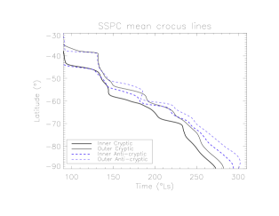
(a) Crocus lines

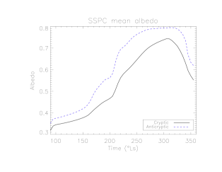
(b) Albedo

Figure 3: Averaged fields interpolated from OMEGA observations for both cryptic and anti-cryptic regions. (a) crocus lines (b) albedo under the aerosols. The interpolated fields are used as an input of the D-frost model.

2.3 D-frost model: daily average sublimated mass model

We use the D-frost model to estimate the daily average $\mathrm{CO_{2}}$ mass surface balance $dM=dM(\lambda,\theta,t)$ for each bin 0.3° latitude, 10° longitude and 5°Ls as described in introduction of section 2. This method estimate the following radiative balance in the visible and IR range:

$$dM=(F_{therm}^{out}-W_{sun}^{in}-W_{scat}^{in}-W_{IR}^{in}-W_{floor}^{in}-F_{cond}^{in})\frac{1}{L_{CO_{2}}}.dt$$ (3)

$F_{therm}^{out}$ represents the thermal energy flux from the surface; $F_{sun}^{in}$ is the direct solar energy absorbed by the surface; $W_{scat}^{in}$ is the solar energy scattered by the atmosphere and absorbed by the surface; $W_{IR}^{in}$ represents the thermal energy emitted by the atmosphere and absorbed by the surface; $W_{floor}^{in}$ is the thermal energy emitted by the neighbouring surface facets and absorbed by the surface; $F_{cond}^{in}$ is the heat flux from the regolith; $L_{CO_{2}}=590\times 10^{3}\>\mathrm{J.kg^{-1}}$ is the latent heat for $\mathrm{CO_{2}}$ sublimation.

The thermal energy flux is estimated with the frost temperature determined by the local pressure of $\mathrm{CO_{2}}$, based on the LMD GCM (Forget et al. (1999)) - calibrated to Viking Lander pressure curves -, scaled to MOLA elevation. The albedo in the thermal infrared domain is assumed to be constant at 0.1 and the emissivity is set to 0.99. Despite these parameters are actually changing in space and time (Eluszkiewicz and Moncet (2003)), a quantitative sensitivity test has shown that it should play a minor role (see section 4.1.6. of Schmidt et al. (2009c)). Also the annual heat wave is neglected to speed up the computation. This energy source has also been demonstrated to be negligible during the sublimation phase (see section 4.1.3. of Schmidt et al. (2009c)). More details about the computation scheme can be found in Schmidt et al. (2009c).

2.3.1 Ar description

We improve the D-frost model by including the effect of the non-condensable gas on the $\mathrm{CO_{2}}$ partial pressure. We use the measurements of Ar by Sprague et al. (2007) to correct for the actual $\mathrm{CO_{2}}$ pressure using the formula:

$$P_{CO_{2}}=P_{GCM}-P_{Ar}$$ (4)

In other words, we use $P_{CO_{2}}$ instead of $P_{GCM}$ in the estimation of surface temperature (see eq. 13 of Schmidt et al. (2009c)).

We use the interpolated albedo field presented in the last section. Altitude and slopes are estimated for each bin averaging a map in stereographic south projection of MOLA data at a resolution of 920.8 m.

2.3.2 Time integration

The total mass sublimated $M$ is estimated by this integral:

$$M=\intop_{-30\text{\textdegree}}^{-90\text{\textdegree}}\intop_{0\text{\textdegree}}^{360\text{\textdegree}}\intop_{t_{0}}^{t_{end}}dM(\lambda,\theta,t).dS.dt$$ (5)

where $t_{0}$ is the beginning of the sublimation (i.e. the first time when $dM<0$), $t_{end}$ is the crocus date (i.e. the time when all the $\mathrm{CO_{2}}$ ice disappears).

We propose two extreme cases for $t_{end}$: the inner crocus date $t_{in}$ and outer the crocus line $t_{out}$. A most realistic case is the decreasing of surface proportion $X=X(t)$ inside each bin from the inner to the outer crocus date. Then eq. 5 becomes:

$$M=\intop_{-30\text{\textdegree}}^{-90\text{\textdegree}}\intop_{0\text{\textdegree}}^{360\text{\textdegree}}\intop_{t_{0}}^{t_{end}}dM(\lambda,\theta,t).X(t).dS.dt$$ (6)

We assume a linear decrease of $X(t)$ with time, from $X=100\%$ at $t_{in}$ to $X=0\%$ at $t_{out}$. Thus the surface proportion can be written:

$$X(t)=\frac{t_{out}-t}{t_{out}-t_{in}}$$ (7)

In the following, this case will be referred to as “linear surface proportion”.

2.4 MOLA height variation

The MOLA observations were performed from February 28, 1999 and June 30, 2001 in a time interval longer than one Martian year (MY 23 and MY24). In this study, we used MOLA data from orbit 10012 to 20327 (from Ls = 103° to 360° in MY23 and then to 190° in MY24). Between Ls=344° in MY23 and Ls=16° in MY24 there are no MOLA data acquired because solar conjunction. This time interval permits to investigate the height changes of the $\mathrm{CO_{2}}$ polar deposits.

To determine the thickness of the $\mathrm{CO_{2}}$ frost layer in different regions as a function of time, it is most important to compute the crossover residuals resulting from subtracting the altitude $h$ of a certain location at some value of Ls to the reference altitude $h_{0}$ at the same location without frost. In this work about the south polar region, the no frost reference altitude is chosen at Ls=300°. We have limited our consideration to a latitudinal band between 50°S and 85°S. Several small areas of about 0.1°-0.2° in longitude and 0.05° in latitude and with enough number of crossovers are then chosen. After computation of the average elevation value of each small area, we calculate the residuals by subtracting the average altitude $h$ of a certain location at some value of Ls to the reference altitude $h_{0}$ at the same location.

3 Results

The total sublimated mass from latitude 50°S to 90°S during the year is about $5.9\times 10^{15}$ kg (fig. 4). The two extreme cases ($4.3\times 10^{15}$ kg for $t_{end}=t_{in}$ and $6.9\times 10^{15}$ for $t_{end}=t_{out}$) are considered as the error bar due to the main uncertainty on the crocus dates such that our estimation is $(5.6\pm 1.3)\times 10^{15}$ kg.

Our estimation is compatible with gravity measurements of Karatekin et al. (2006) ($\sim 6\times 10^{15}$ kg), GRS estimation from Kelly et al. (2006) ($6\times 10^{15}$ kg) and HEND analysis provided by Litvak et al. (2007) ($(6.1\pm 0.6)\times 10^{15}$ kg). Since our calculations are done in the domain 50°S to 90°S only and since we found the same numbers than other methods based on a global approach, it suggests that the $\mathrm{CO_{2}}$ mass condensed at latitude lower than 50S is negligible.

The GCM by Forget et al. (1999), calibrated by the pressure variation measurement from Viking, give also an estimate of the total SSPC of $6.9\times 10^{15}$ kg, slightly higher than our estimation. The pattern of the total sublimated mass $M$ along time (fig 4) is compatible with the GCM (Forget et al. (1999)) although the starting of sublimation seems to be slightly earlier for the D-frost model. Nevertheless, there is a good agreement about the end of sublimation: around Ls=270°. The shift in the beginning of sublimation can be explained by the integration method. In this study, we integrate spatially the $\mathrm{CO_{2}}$ mass that is subliming, independently of the condensation domain. In the GCM integrations (Forget et al. (1999)), the whole SSPC spatial domain is covered: subliming and condensing $\mathrm{CO_{2}}$. At Ls=90°, the average SSPC balance measured by the GCM is in accumulation due to the geographic polar region. Our integration shows already the sublimation that occurs at low latitude.

It is not possible to extend our calculation to the condensation domain because one energy source is missing: heat conducted in the soil (Haberle et al. (2008)), which is no more negligible for the accumulation period (Schmidt et al. (2009c)). Our estimation is limited in the domain latitude 50°S to 90°S because for lower latitudes, $\mathrm{CO_{2}}$ frost may be possible only with an apparent albedo below our threshold (0.3). Nevertheless, MOC observations shows seasonal frost at lower latitude suspected to be $\mathrm{CO_{2}}$ ice (Schorghofer and Edgett (2006)). These condensates could be also predicted with D-frost using lower albedo and the shadowing effect at lower scale and would be an interesting point for the future. The good agreement between our mass balance and direct mass measurements suggests that the low latitude frost mass is negligible at first order.

If the Ar is well mixed in the south polar region, the effect on the temperature and thus on the total sublimated mass is below 1%.

Figure 4: Total cumulative sublimated mass estimated by the D-frost model using OMEGA inputs compared with GCM (Forget et al. (1999)). Please note that a negative balance corresponds to surface mass loss (surface convention).

Figure 5 shows the integration of the SSPC sublimation for the two regions. The main conclusion is that despite the asymmetry of crocus lines and albedo, the sublimated mass seems to be symmetric around the geographic pole. The difference reach 20.5 % (12.5 % for $t_{end}=t_{in}$, 31.2 % for $t_{end}=t_{out}$). To compile all errors, we estimate roughly that the mass difference is $22\%\pm 9$. This conclusion confirms that the condensation phases are not equivalent during the polar night for both cryptic and anti-cryptic sectors in contrary of our previous work (Schmidt et al. (2009c)) argued only on four latitude points. There is a significant higher mass condensed in the anti-cryptic region, probably due to snow event, as previously suggested Colaprete et al. (2005); Giuranna et al. (2008).

Assuming a density of 920 kg.$\mathrm{m}^{-3}$ (as determined by Smith et al. (2001)), the estimated maximum height from the D-frost model reach 0.32 m (0.21 m for $t_{end}=t_{in}$, 0.40 m for $t_{end}=t_{out}$) in the cryptic region and 0.41 m (0.31 m for $t_{end}=t_{in}$, 0.46 m for $t_{end}=t_{out}$) in the anti-cryptic region (see fig. 5). We compile the errors to estimate the height $0.31\pm 0.10$ m for the cryptic region and $0.38\pm 0.08$ m for the anti-cryptic region. In comparison, the direct MOLA height measurements are $0.37\pm 0.08$ m for the cryptic region and $0.35\pm 0.08$ m for the anti-cryptic region at Ls=150°. At first order, absolute results from both methods are compatible with a difference below the error bar (see fig. 5). The difference anti-cryptic/cryptic in the MOLA data is significant at Ls=210° and Ls=240° in agreement with the D-frost model, when the mass ratio anti-cryptic/cryptic is the highest. At this time period, the MOLA height measurement is higher than the D-frost estimation probably due to a $\mathrm{CO_{2}}$ bulk density lower than 920 kg.$\mathrm{m}^{-3}$ as suggested by Aharonson et al. (2004); Giuranna et al. (2007b); Matsuo and Heki (2009).

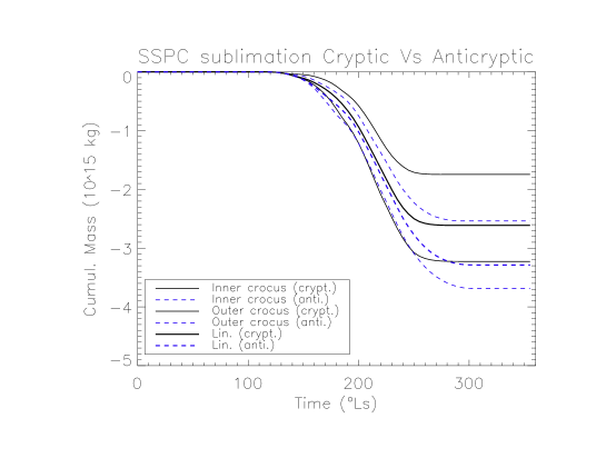
(a) Integrated mass sublimation

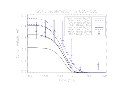
(b) Integrated mass sublimation

Figure 5: Total sublimated $\mathrm{CO_{2}}$ mass (a) and total sublimated mass $\mathrm{CO_{2}}$ height (b) for both cryptic and anti-cryptic region (surface convention) assuming a density of 920 kg.$\mathrm{m}^{-3}$ (as determined by Smith et al. (2001)) compared to MOLA height change.

During the first phase, the sublimation is nearly symmetric with a significant higher sublimation in the cryptic region for the time period Ls=180° to 220° (see fig. 6(a) and (b)). This corresponds to appearance of the low albedo cryptic region (Kieffer et al. (2000); Piqueux et al. (2003); Langevin et al. (2007)) that absorbs and sublimates faster.

After Ls=220° the average anti-cryptic sector is subliming stronger with a maximum difference of $1.0\times 10^{8}$ kg.$\mathrm{s}^{-1}$ (see fig. 6(a) and (b)) despite a maximum sublimation rate locally in the cryptic region. This is due to the fact that the effect of difference in surface cover is stronger than the effect of difference in albedo. At Ls=230, the ratio surface ratio is $R_{surf}=\frac{Surface\>anti-cryptic}{Surface\>cryptic}=1.55$ (see fig. 3 (a)) and the absorbance ratio is $R_{abs}=\frac{1-Albedo\>anti-cryptic}{1-Albedo\>cryptic}=0.71$ (see fig. 3 (b)). If we simplify eq. 2 and only keep the direct sunlight term $W_{sun}^{in}$, the sublimation mass rates ratio can be estimated $R_{mass}=\frac{Mass\>anti-cryptic}{Mass\>cryptic}=R_{surf}.R_{abs}=1.11$, in agreement with our results (see fig. 6(a) and (b)). With this simple calculation, we demonstrate that after Ls=220° the anti-cryptic region is sublimating faster due to the fact that the SSPC recession is asymmetric, i.e.: the anti-cryptic region reaches the outer crocus line before the cryptic region.

Two phases are not balanced such that the total mass is different for both regions, with 20% more mass in the anti-cryptic region, arguing for more snow precipitation during winter time (Colaprete et al. (2005); Giuranna et al. (2008)). If the resulting material in the anti-cryptic region, more concentrated in snow, has significant lower emissivity, it could also condensate slower. If this process occurs during the polar night, 20 % is the minimum snow content. During winter time, “cold spots” has been observed since the 70’s and been interpreted as clouds or fresh snow at the surface (Kieffer et al. (1977); Forget (1998); Ivanov and Muhleman (2001)). Recent studies showed that the “cold spots” dynamic in thermal infrared range is as short as 5 Julian days (Cornwall and Titus (2009); Cornwall and N. (2010)) suggesting that metamorphism is very active and very fast on Mars. Thus the $\mathrm{CO_{2}}$ emissivity is not likely to be lower than 0.9 during a significant period of time.

In conclusion, our estimates indicate that the sublimation flux is modulated by the local properties of the cryptic/anti-cryptic regions and in particular the crocus date. Schmidt et al. (2009c) conclusions are still valid: albedo is controlling the SSPC sublimation but once there is no $\mathrm{CO_{2}}$ ice anymore it is obvious that the sublimation stops.

(a) Absolute sublimation rates

(b) Sublimation rates difference

Figure 6: Sublimated Mass and within the cryptic region and the anti-cryptic region. Note that the sublimated mass is a negative quantity so that when this difference is positive, the cryptic region is subliming faster than the anti-cryptic region (surface convention).

4 Ar dilution in the south polar vortex

Since SSPC is sublimating, the atmosphere is pumped up and rebalanced by mass transfer at global scale (Hourdin et al. (1995)). This mass transfer lead also to a differential dilution of the minor non-condensable gas that acts like tracer of the phenomena. In addition to the sublimating SSPC, air mass coming from lower latitudes could enter the polar vortex and dilute the local air (Colaprete et al. (2008)). Using a box modeling, we propose here to estimate the relevant quantity for this system: $\mathcal{F}$ the advection flux and compare it to $Q$ the sublimation flux.

Modeling the geophysical system by boxes is a very convenient approach to understand the natural phenomena in a simple manner (Albarède (2003)). We propose to model the martian atmosphere using 3 boxes: the south polar deposits (SSPC), the polar atmosphere and the martian atmosphere as a whole (see fig 7).

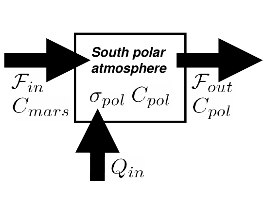
Figure 7: Schema of the box modeling with $\mathcal{F}$ the advection flux, $Q$ the sublimation flux, $\sigma_{pol}$ the mass of the polar atmosphere column and $C$ the mixing ratio of non condensable gas, such Ar.

$\mathrm{CO_{2}}$ balance

We could write the mass balance of the polar atmosphere of $\mathrm{CO_{2}}$ as:

$$\frac{d\sigma_{pol}}{dt}=Q_{in}+\mathcal{F}_{in}-\mathcal{F}_{out}$$ (8)

With $\sigma_{pol}=\frac{M_{pol}}{S_{pol}}$ the mass of the polar atmosphere column by surface unit (in $\mathrm{kg.m^{-2}}$), the incoming flux from the sublimation $Q_{in}=dM$ estimated in the last section in atmosphere sign convention (in $\mathrm{kg.m^{-2}.s^{-1}}$), $\mathcal{F}_{in}$ and $\mathcal{F}_{out}$ are respectively the incoming and outcoming advection fluxes (in $\mathrm{kg.m^{-2}.s^{-1}}$).

We assume that the system is in steady state $\frac{d\sigma_{pol}}{dt}=0$ such that the incoming fluxes exactly compensate the outgoing flux: $Q_{in}+\mathcal{F}_{in}=\mathcal{F}_{out}$. In other terms, we suppose that the mass rebalance time of the atmosphere is much lower than the typical time of the non-condensable gas balance.

Non-condensable species balance

We could also write the mass balance of the minor non condensable species, assuming that they are in homogeneous mixing within all boxes:

$$\sigma_{pol}.\frac{dC_{pol}}{dt}=\mathcal{F}_{in}.C_{mars}-\mathcal{F}_{out}.C_{pol}$$ (9)

With $C_{pol}$ and $C_{mars}$, the mixing ratio of the non condensable gas in the polar region respectively in the whole Martian atmosphere. We solve this equation using the following numerical solution:

$$C_{pol}(t+\Delta t)=C_{pol}(t).\left(1-\frac{\mathcal{F}_{in}}{\sigma_{pol}}.\Delta t-\frac{Q_{in}}{\sigma_{pol}}.\Delta t\right)+C_{mars}.\frac{\mathcal{F}_{in}}{\sigma_{pol}}.\Delta t$$ (10)

For the convenience, we use a time step $\Delta t=1s$.

Measurements of the Ar in the south polar atmosphere have been done by the GRS instrument (Sprague et al. (2004, 2007)). During the time period of sublimation in the south polar region (Ls=110-350), we estimate the decrease of Ar using eq. 10. We set the initial value of Ar abundance $C_{pol}(t=110\text{\textdegree}Ls)=3.89$% as measured by GRS. We use the commonly used value of the Martian mixing ratio $C_{mars}=1.6$% in agreement with Viking Lander 2 measurements (Owen et al. (1977)).

Minor species abundances evolution with time are plotted in fig. 8, for different values of $\mathcal{F}_{in}$: 0, $4.10^{-6}$, $8.10^{-6}$ and $20.10^{-6}$ $\mathrm{kg.m^{-2}.s^{-1}}$. The mixing ratio evolution decreases with time to reach a minimum around Ls=250 and then increases again. The first decrease is due to the sublimation of the seasonal frost, free of non-condensable gas. In addition, the advection flux dilutes Ar with a higher $\mathcal{F}_{in}$ leading to a faster dilution. The increase in second step is due to the injection of the Martian air, slightly enriched in Ar compared to the local polar air. The rate of increase is higher when $\mathcal{F}_{in}$ is faster.

By matching GRS data with our box model, we estimate that the flux $\mathcal{F}_{in}\simeq 4.10^{-6}\mathrm{\>kg.m^{-2}.s^{-1}}$. This value has the same order of magnitude as the mean value of the sublimation flux $\left\langle Q_{in}\right\rangle=6.7\times 10^{-6}\mathrm{\>kg.m^{-2}.s^{-1}}$. This result suggests that the air mass entering the south polar vortex during the recession phase is of the same order than the sublimated mass. Thus the local difference in $Q_{in}$ due to asymmetry should lead to non-negligible effect on the vortex dynamic, especially after Ls=220° (see fig. 6).

Future studies using GCM or local climate model have to be conducted to study the actual dynamical effect of the asymmetry in sublimation. One particular attention should be drawn on the dilution factor regarding the dynamics in the cryptic vs anti-cryptic region. Some regional differences should be pointed out, as suggested by GRS (Sprague et al. (2007)).

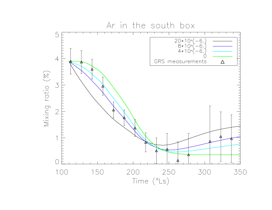
Figure 8: Estimation of $C_{pol}$ as a function of time in comparison with actual Ar measurements in the South Polar atmosphere. Lines represent the solution of our box modeling (eq. 10) for four cases: $\mathcal{F}_{in}=0$, $10^{-5}$, $5.10^{-5}$ and $10^{-4}$ $\mathrm{kg.m^{-2}.s^{-1}}$. Triangles are Ar observations of the GRS instruments (Sprague et al. (2007)) for the whole south polar region.

5 Conclusions

We estimate the $\mathrm{CO_{2}}$ mass balance of the SSPC using the D-frost model and estimate the total sublimated mass to be around $(5.6\pm 1,3)\times 10^{15}$ kg which is compatible with gravity measurements (Karatekin et al. (2006)), with measurements by gamma ray and neutron spectroscopy (Litvak et al. (2006); Kelly et al. (2006)) and with previous GCM studies (Forget et al. (1999); Kelly et al. (2006)). This agreement validates our current approach.

The effect of the Ar content, in the case of a well mixed atmosphere is below 1% on the total sublimated mass. A more realistic case of denser Ar enriched air in the bottom part of the atmosphere should be studied in the future.

We show that the SSPC is not symmetric in mass around the geographic pole, i.e.: the cryptic and anti-cryptic regions have an accumulated mass with a difference in order of $22\pm 9$ %. in favour of the anti-cryptic region. Previous studies suggested that in addition to direct condensation, during the southern fall and winter seasons, snow precipitation is more intense in the anti-cryptic region than in the cryptic one (Colaprete and Toon (2002); Giuranna et al. (2008)). Our results show that, the actual mass deposited (possibly as snow) should be in order of 20 %. This conclusion is still valid if the $\mathrm{CO_{2}}$ emissivity has regional and/or temporal variations within the range 0.9 to 1 during the spring and summer, as observed by TES (Eluszkiewicz and Moncet (2003)) ans supported by fast $\mathrm{CO_{2}}$ metamorphism (Cornwall and N. (2010)). The previous estimation on small regions of interests (ROI) by Kieffer et al. (2000) was 852 $\mathrm{kg.m}^{-1}$ in the “cryptic” ROI and 841$\mathrm{kg.m}^{-1}$ in the “bright cap” ROI. The difference is probably due to the crocus date measurement that is delayed for OMEGA in comparison to TES. In case of subpixel mixing, due to the thermal emission dependence on the temperature at power four, bare soil is dominating in the thermal infrared. This effect is not present in near infrared domain and the mixing is really linear. Further studies should be done to precisely compare visible, near infrared and thermal infrared datasets.

From Ls=180° to 220°, we point out that the cryptic region is sublimating slightly stronger than the anti-cryptic region. In the second phase, anti-cryptic region sublimation is dominating with a maximum difference in sublimation of $1.0\times 10^{8}$ kg.$\mathrm{s}^{-1}$. This results is compatible with the MOLA height measurements difference that reach a maximum for Ls=210°-240°.

We use a simple box model to fit the GRS measurements of Ar and estimate that the atmosphere advection flux entering the south polar vortex is similar to the flux from the sublimating SSPC.

More precise studies on atmosphere dynamics and minor species concentration should be carried out with a GCM or a local scale climate model. At present time, SSPC albedo is a constant parameter in any GCM. Future studies should be done to include the SSPC asymmetry of albedo leading to an asymmetry of sublimation in order to simulate realistic dynamics and dilution factors. Those results will have to be compared to the atmospheric observations of pressure (for instance using the method proposed by Forget et al. (2007); Spiga et al. (2007)) and minor species concentration (using gamma rays, i.e.: Sprague et al. (2004), optical measurements on the ground i.e: Encrenaz et al. (2005), or orbiters i.e.: Melchiorri et al. (2007)).

In particular, future local climate studies should explain the actually asymmetric Ar enrichment (Sprague et al. (2004)) that could play an indirect role in the stability of the SSPC itself. If the atmosphere is locally enriched in Ar, the partial pressure of $\mathrm{CO_{2}}$ is lower and then $\mathrm{CO_{2}}$ ice stability is lower (Forget et al. (2008)).

6 Acknowledgments

This work has been supported by a contract with CNES through its ’Systeme Solaire’ program. We thank the OMEGA and MOLA teams for data management. We also thank Mathieu Vincendon providing the SSPC reflectance map, under the aerosols. Finally, we are grateful to two anonymous reviewers for their helpful comments.

References

- Aharonson et al. (2004) Aharonson, O., Zuber, M. T., Smith, D. E., Neumann, G. A., Feldman, W. C., Prettyman, T. H., May 2004. Depth, distribution, and density of CO2 deposition on Mars. Journal of Geophysical Research (Planets) 109, 5004–+.
- Albarède (2003) Albarède, F., 2003. Geochemistry : An Introduction. Cambridge University Press.
- Bibring et al. (2004) Bibring, J.-P., Soufflot, A., Berthé, M., Langevin, Y., Gondet, B., Drossart, P., Bouyé, M., Combes, M., Puget, P., Semery, A., Bellucci, G., Formisano, V., Moroz, V., Kottsov, V., Bonello, G., Erard, S., Forni, O., Gendrin, A., Manaud, N., Poulet, F., Poulleau, G., Encrenaz, T., Fouchet, T., Melchiori, R., Altieri, F., Ignatiev, N., Titov, D., Zasova, L., Coradini, A., Capacionni, F., Cerroni, P., Fonti, S., Mangold, N., Pinet, P., Schmitt, B., Sotin, C., Hauber, E., Hoffmann, H., Jaumann, R., Keller, U., Arvidson, R., Mustard, J., Forget, F., Aug. 2004. OMEGA: Observatoire pour la Minéralogie, l’Eau, les Glaces et l’Activité. ESA SP-1240: Mars Express: the Scientific Payload, pp. 37–49.
- Colaprete et al. (2005) Colaprete, A., Barnes, J. R., Haberle, R. M., Hollingsworth, J. L., Kieffer, H. H., Titus, T. N., May 2005. Albedo of the south pole on Mars determined by topographic forcing of atmosphere dynamics. Nature 435, 184–188.
-
Colaprete et al. (2008)
Colaprete, A., Barnes, J. R., Haberle, R. M., Montmessin, F., Feb. 2008. Co2
clouds, cape and convection on mars: Observations and general circulation
modeling. Planetary and Space Science 56 (2), 150–180.
URL http://www.sciencedirect.com/science/article/B6V6T-4PKX%BT3-1/2/dfd675ef50bb83015599c6bd3c714ed6 - Colaprete and Toon (2002) Colaprete, A., Toon, O. B., Jul. 2002. Carbon dioxide snow storms during the polar night on Mars. Journal of Geophysical Research (Planets) 107, 5–1.
- Cornwall and N. (2010) Cornwall, C., N., T. T., 2010. A comparison of martain north and south polar cold spots and the long-term effects of the 2001 global dust storm. J. Geophys. Res. in press.
- Cornwall and Titus (2009) Cornwall, C., Titus, T. N., Feb. 2009. Spatial and temporal distributions of Martian north polar cold spots before, during, and after the global dust storm of 2001. Journal of Geophysical Research (Planets) 114, 2003–+.
-
Eluszkiewicz and
Moncet (2003)
Eluszkiewicz, J., Moncet, J.-L., Dec. 2003. A coupled microphysical/radiative
transfer model of albedo and emissivity of planetary surfaces covered by
volatile ices. Icarus 166 (2), 375–384.
URL http://www.sciencedirect.com/science/article/B6WGF-49V1%%****␣Schmidt_AsymetricReleaseSSPC_elsevier-submit3_v2.bbl␣Line␣75␣****DPH-3/2/12ed8d86bc224511b0d6f7ee29500ac6 - Encrenaz et al. (2005) Encrenaz, T., Bézard, B., Owen, T., Lebonnois, S., Lefèvre, F., Greathouse, T., Richter, M., Lacy, J., Atreya, S., Wong, A. S., Forget, F., Dec. 2005. Infrared imaging spectroscopy of Mars: H2O mapping and determination of CO2 isotopic ratios. Icarus 179, 43–54.
- Forget (1998) Forget, F., 1998. Mars CO2 ice polar caps. In: Schmitt, B., de Bergh, C., Festou, M. (Eds.), Solar System Ices. Vol. 227 of Astrophysics and Space Science Library. Kluwer, pp. 477–507.
- Forget et al. (1999) Forget, F., Hourdin, F., Fournier, R., Hourdin, C., Talagrand, O., Collins, M., Lewis, S. R., Read, P. L., Huot, J.-P., Oct. 1999. Improved general circulation models of the Martian atmosphere from the surface to above 80 km. Journal of Geophysical Research (Planets) 104, 24155–24176.
- Forget et al. (1998) Forget, F., Hourdin, F., Talagrand, O., Feb. 1998. CO2 Snowfall on Mars: Simulation with a General Circulation Model. Icarus 131, 302–316.
- Forget et al. (2008) Forget, F., Millour, E., Montabone, L., Lefevre, F., Nov. 2008. Non Condensable Gas Enrichment and Depletion in the Martian Polar Regions. LPI Contributions 1447, 9106–+.
- Forget et al. (2007) Forget, F., Spiga, A., Dolla, B., Vinatier, S., Melchiorri, R., Drossart, P., Gendrin, A., Bibring, J.-P., Langevin, Y., Gondet, B., Aug. 2007. Remote sensing of surface pressure on Mars with the Mars Express/OMEGA spectrometer: 1. Retrieval method. Journal of Geophysical Research (Planets) 112, 8–+.
-
Giuranna et al. (2007a)
Giuranna, M., Formisano, V., Grassi, D., Maturilli, A., Jul.
2007a. Tracking the edge of the south seasonal polar cap of
mars. Planetary and Space Science 55 (10), 1319–1327.
URL http://www.sciencedirect.com/science/article/B6V6T-4MS9%RGP-1/2/5e2cde3a3b8173badddefababaeaa1f0 -
Giuranna et al. (2008)
Giuranna, M., Grassi, D., Formisano, V., Montabone, L., Forget, F., Zasova, L.,
Oct. 2008. Pfs/mex observations of the condensing co2 south polar cap of
mars. Icarus 197 (2), 386–402.
URL http://www.sciencedirect.com/science/article/B6WGF-4SPY%KJM-1/2/61736d61880cf7c503ff493adcc83204 -
Giuranna et al. (2007b)
Giuranna, M., Hansen, G., Formisano, V., Zasova, L., Maturilli, A., Grassi, D.,
Ignatiev, N., Jul. 2007b. Spatial variability, composition and
thickness of the seasonal north polar cap of mars in mid-spring. Planetary
and Space Science 55 (10), 1328–1345.
URL http://www.sciencedirect.com/science/article/B6V6T-4ND0%RT5-1/2/296230f162e6ab90e6d175919d2e324c - Haberle et al. (2008) Haberle, R. M., Forget, F., Colaprete, A., Schaeffer, J., Boynton, W. V., Kelly, N. J., Chamberlain, M. A., Feb. 2008. The effect of ground ice on the Martian seasonal CO2 cycle. Planetary and Space Science 56, 251–255.
- Hapke (1993) Hapke, B., 1993. Theory of reflectance and emittance spectroscopy. Topics in Remote Sensing, Cambridge, UK: Cambridge University Press.
- Hourdin et al. (1995) Hourdin, F., Forget, F., Talagrand, O., Mar. 1995. The sensitivity of the Martian surface pressure and atmospheric mass budget to various parameters: A comparison between numerical simulations and Viking observations. Journal of Geophysical Research (Planets) 100, 5501–5523.
- Ivanov and Muhleman (2001) Ivanov, A. B., Muhleman, D. O., Nov. 2001. Cloud Reflection Observations: Results from the Mars Orbiter Laser Altimeter. Icarus 154, 190–206.
-
Jian and Ip (2009)
Jian, J.-J., Ip, W.-H., Jan. 2009. Seasonal patterns of condensation and
sublimation cycles in the cryptic and non-cryptic regions of the south pole.
Advances in Space Research 43 (1), 138–142.
URL http://www.sciencedirect.com/science/article/B6V3S-4SGD%4WD-1/2/6db9a653ed786828772a3eb7a319b2d7 - Karatekin et al. (2006) Karatekin, Ö., Van Hoolst, T., Dehant, V., Jun. 2006. Martian global-scale CO2 exchange from time-variable gravity measurements. Journal of Geophysical Research (Planets) 111, 6003–+.
- Kelly et al. (2006) Kelly, N. J., Boynton, W. V., Kerry, K., Hamara, D., Janes, D., Reedy, R. C., Kim, K. J., Haberle, R. M., Dec. 2006. Seasonal polar carbon dioxide frost on Mars: CO2 mass and columnar thickness distribution. Journal of Geophysical Research (Planets) 111, 3–+.
- Kieffer (2007) Kieffer, H. H., Aug. 2007. Cold jets in the Martian polar caps. Journal of Geophysical Research (Planets) 112, 8005–+.
-
Kieffer et al. (2006)
Kieffer, H. H., Christensen, P. R., Titus, T. N., Aug. 2006. Co2 jets
formed by sublimation beneath translucent slab ice in mars’ seasonal south
polar ice cap. Nature 442 (7104), 793–796.
URL http://dx.doi.org/10.1038/nature04945 - Kieffer et al. (1977) Kieffer, H. H., Martin, T. Z., Peterfreund, A. R., Jakosky, B. M., Miner, E. D., Palluconi, F. D., Sep. 1977. Thermal and albedo mapping of Mars during the Viking primary mission. Journal of Geophysical Research (Planets) 82, 4249–4291.
- Kieffer et al. (2000) Kieffer, H. H., Titus, T. N., Mullins, K. F., Christensen, P. R., Apr. 2000. Mars south polar spring and summer behavior observed by TES: Seasonal cap evolution controlled by frost grain size. Journal of Geophysical Research (Planets) 105, 9653–9700.
- Langevin et al. (2007) Langevin, Y., Bibring, J.-P., Montmessin, F., Forget, F., Vincendon, M., Douté, S., Poulet, F., Gondet, B., Jul. 2007. Observations of the south seasonal cap of Mars during recession in 2004-2006 by the OMEGA visible/near-infrared imaging spectrometer on board Mars Express. Journal of Geophysical Research (Planets) 112, 8–+.
-
Langevin et al. (2006)
Langevin, Y., Douté, S., Vincendon, M., Poulet, F., Bibring, J.-P., Gondet,
B., Schmitt, B., Forget, F., Aug. 2006. No signature of clear co2 ice
from the ‘cryptic’ regions in mars’ south seasonal polar cap. Nature
442 (7104), 790–792.
URL http://dx.doi.org/10.1038/nature05012 - Leighton and Murray (1966) Leighton, R. R., Murray, B. C., Jul. 1966. Behavior of carbon dioxide and other volatiles on Mars. Science 153, 136–144.
- Lindner (1993) Lindner, B. L., Feb. 1993. The hemispherical asymmetry in the Martian polar caps. Journal of Geophysical Research (Planets) 98, 3339–3344.
- Litvak et al. (2007) Litvak, M. L., Mitrofanov, I. G., Kozyrev, A. S., Sanin, A. B., Tretyakov, V. I., Boynton, W. V., Kelly, N. J., Hamara, D., Saunders, R. S., Feb. 2007. Long-term observations of southern winters on Mars: Estimations of column thickness, mass, and volume density of the seasonal CO2 deposit from HEND/Odyssey data. Journal of Geophysical Research (Planets) 112, 3–+.
- Litvak et al. (2006) Litvak, M. L., Mitrofanov, I. G., Kozyrev, A. S., Sanin, A. B., Tretyakov, V. I., Boynton, W. V., Kelly, N. J., Hamara, D., Shinohara, C., Saunders, R. S., Jan. 2006. Comparison between polar regions of Mars from HEND/Odyssey data. Icarus 180, 23–37.
-
Matsuo and Heki (2009)
Matsuo, K., Heki, K., Jul. 2009. Seasonal and inter-annual changes of volume
density of martian co2 snow from time-variable elevation and gravity. Icarus
202 (1), 90–94.
URL http://www.sciencedirect.com/science/article/B6WGF-4VS4%0BF-3/2/0b319f0d9c9fd76260beb2ea1164e0e8 -
Melchiorri et al. (2007)
Melchiorri, R., Encrenaz, T., Fouchet, T., Drossart, P., Lellouch, E., Gondet,
B., Bibring, J.-P., Langevin, Y., Schmitt, B., Titov, D., Ignatiev, N., Feb.
2007. Water vapor mapping on mars using omega/mars express. Planetary and
Space Science 55 (3), 333–342.
URL http://www.sciencedirect.com/science/article/B6V6T-4KST%3NG-5/2/408bf3ecd2f2bd46cccbc78575f37d45 - Owen et al. (1977) Owen, T., Biemann, K., Biller, J. E., Lafleur, A. L., Rushneck, D. R., Howarth, D. W., Sep. 1977. The composition of the atmosphere at the surface of Mars. Journal of Geophysical Research (Planets) 82, 4635–4639.
- Paige and Ingersoll (1985) Paige, D. A., Ingersoll, A. P., Jun. 1985. Annual heat balance of Martian polar caps - Viking observations. Science 228, 1160–1168.
- Piqueux et al. (2003) Piqueux, S., Byrne, S., Richardson, M. I., Aug. 2003. Sublimation of Mars’s southern seasonal CO2 ice cap and the formation of spiders. Journal of Geophysical Research (Planets) 108, 3–1.
- Pollack et al. (1990) Pollack, J. B., Haberle, R. M., Schaeffer, J., Lee, H., Feb. 1990. Simulations of the general circulation of the Martian atmosphere. I - Polar processes. Journal of Geophysical Research (Planets) 95, 1447–1473.
- Schmidt et al. (2007) Schmidt, F., Douté, S., Schmitt, B., 2007. Wavanglet: An efficient supervised classifier for hyperspectral images. Geoscience and Remote Sensing, IEEE Transactions on 45 (5), 1374–1385.
- Schmidt et al. (2009a) Schmidt, F., Doute, S., Schmitt, B., Langevin, Y., Bibring, J.-P., the OMEGA Team, septembre 2009a. Slab ice in the seasonal south polar cap of Mars. In: European Planetary Science Congress (EuroPlanet), Potsdam, Germany, 13/09/09-18/09/09. Vol. 4. EuroPlanet, http://www.europlanet-eu.org, p. (electronic medium).
- Schmidt et al. (2009b) Schmidt, F., Douté, S., Schmitt, B., the OMEGA Team., 2009b. Physical state of co2 ice in the seasonal south polar cap. Icarus (in preparation).
-
Schmidt et al. (2009c)
Schmidt, F., Douté, S., Schmitt, B., Vincendon, M., Bibring,
J.-P., Langevin, Y., Apr. 2009c. Albedo control of seasonal
south polar cap recession on mars. Icarus 200 (2), 374–394.
URL http://www.sciencedirect.com/science/article/B6WGF-4V76%270-1/2/60231d55061d19abebb5344bd9e40e2b - Schmidt et al. (2008) Schmidt, F., Schmitt, B., Douté, S., Forget, F., Langevin, Y., Bibring, J., Omega Team, Nov. 2008. Asymmetric Release of CO2 During Southern Spring. LPI Contributions 1447, 9003–+.
- Schorghofer and Edgett (2006) Schorghofer, N., Edgett, K. S., Feb. 2006. Seasonal surface frost at low latitudes on Mars. Icarus 180, 321–334.
- Smith et al. (2001) Smith, D. E., Zuber, M. T., Neumann, G. A., Dec. 2001. Seasonal Variations of Snow Depth on Mars. Science 294, 2141–2146.
- Spiga et al. (2007) Spiga, A., Forget, F., Dolla, B., Vinatier, S., Melchiorri, R., Drossart, P., Gendrin, A., Bibring, J.-P., Langevin, Y., Gondet, B., Aug. 2007. Remote sensing of surface pressure on Mars with the Mars Express/OMEGA spectrometer: 2. Meteorological maps. Journal of Geophysical Research (Planets) 112, 8–+.
- Sprague et al. (2007) Sprague, A. L., Boynton, W. i. V., Kerry, K. E., Janes, D. M., Kelly, N. J., Crombie, M. K., Nelli, S. M., Murphy, J. R., Reedy, R. C., Metzger, A. E., 2007. Mars atmospheric argon: Tracer for understanding martian atmospheric circulation and dynamics. Journal of Geophysical Research (Planets) 112, 15–+.
- Sprague et al. (2004) Sprague, A. L., Boynton, W. V., Kerry, K. E., Janes, D. M., Hunten, D. M., Kim, K. J., Reedy, R. C., Metzger, A. E., Nov. 2004. Mars’ South Polar Ar Enhancement: A Tracer for South Polar Seasonal Meridional Mixing. Science 306, 1364–1367.
- Titus et al. (2008) Titus, T. N., Calvin, W. M., Kieffer, H. H., Langevin, Y., Prettyman, T. H., Jul. 2008. Martian polar processes. Ch. 25, pp. 578–+.
-
Vincendon et al. (2008)
Vincendon, M., Langevin, Y., Poulet, F., Bibring, J.-P., Gondet, B., Jouglet,
D., Aug. 2008. Dust aerosols above the south polar cap of mars as seen by
omega. Icarus 196 (2), 488–505.
URL http://www.sciencedirect.com/science/article/B6WGF-4RV1%7PY-2/1/781d47cebdea184a353f89f9a98b3e35 - Warren et al. (1990) Warren, S. G., Wiscombe, W. J., Firestone, J. F., Aug. 1990. Spectral albedo and emissivity of CO2 in Martian polar caps - Model results. Journal of Geophysical Research (Planets) 95, 14717–14741.
-
Wood and Paige (1992)
Wood, S. E., Paige, D. A., Sep. 1992. Modeling the martian seasonal co2 cycle
1. fitting the viking lander pressure curves. Icarus 99 (1), 1–14.
URL http://www.sciencedirect.com/science/article/B6WGF-470F%41G-7D/2/96bed1f6e592f4e45ce3720b8b0ecfd0