Scaling Behaviors of Weighted Food Webs as Energy Transportation Networks

Abstract

Food webs can be regarded as energy transporting networks in which the weight of each edge denotes the energy flux between two species. By investigating 21 empirical weighted food webs as energy flow networks, we found several ubiquitous scaling behaviors. Two random variables $A_{i}$ and $C_{i}$ defined for each vertex $i$, representing the total flux (also called vertex intensity) and total indirect effect or energy store of $i$, were found to follow power law distributions with the exponents $\alpha\approx 1.32$ and $\beta\approx 1.33$, respectively. Another scaling behavior is the power law relationship, $C_{i}\sim A_{i}^{\eta}$, where $\eta\approx 1.02$. This is known as the allometric scaling power law relationship because $A_{i}$ can be treated as metabolism and $C_{i}$ as the body mass of the sub-network rooted from the vertex $i$, according to the algorithm presented in this paper. Finally, a simple relationship among these power law exponents, $\eta=(\alpha-1)/(\beta-1)$, was mathematically derived and tested by the empirical food webs.

1 Introduction

Scientists look for universal patterns of complex systems because such invariant features may help to unveil the principles of system organization(Waldrop, 1992). Complex network studies can not only provide a unique viewpoint of nature and society but also reveal ubiquitous patterns, e.g., small world and scale free, characteristic of various complex systems(Watts and Strogatz, 1998; Albert and Barabasi, 2002). However, ecological studies have shown that binary food webs, which depict trophic interactions in ecosystems, refuse to become part of the small world and scale free networks family (Montoya and Sole, 2002; Dunne et al., 2002). Although some common features, including ”two degrees separation”, which means the very small average distance, are shared among food webs (Williams et al., 2002), other meaningful attributes such as degree distribution and clustering coefficient change with the size and complexity (connectance) of the network (Dunne et al., 2002).

Weight information of complex networks such as air traffic network or metabolism networks, etc., can reveal more unique patterns and features that are never found in binary relationships(Barrat et al., 2004; Almaas et al., 2004; Montis et al., 2007). Food web weights have two different, yet correlated, meanings in ecology. One is the strength of the trophic interaction(Emmerson and Raffaelli, 2004; Berlow et al., 2004); the other is the amount of energy flow. They are correlated because interaction strength is the per capita measure of energy flow. Interaction strength-based weighted food webs exhibit new features such as a relationship between predator-prey body size ratio and interaction strength (McCann et al., 1998; Wootton, 2002; Berlow et al., 2004).

Additionally, weights of food webs can also be denoted as the total amount of energy flow between two species when the whole system is in the steady state. Studies of energy flow networks in ecosystems have a long history (Odum, 1988; Finn, 1976; Szyrmer and Ulanowicz, 1987; Higashi, 1986; Baird and Ulanowicz, 1989; Higashi et al., 1993; Patten, 1981, 1982). Many systematic indicators were designed to depict the macro-state of energy flow in ecosystem (Fath and Patten, 1999; Fath et al., 2001), of which some can not only reflect the direct energy flows between species but also indirect effects and inter-dependence of species(Fath and Patten, 1999; Finn, 1976). Although some important discoveries were made about the general structure and function of ecological networks(Fath and B.C., 1998; Hannon, 1973; Levine, 1980; Hannon, 1986; Patten, 1985; Ulanowicz, 1986, 1997), few focus on power law distributions and relations(Ulanowicz and Wolff., 1990).

Allometric scaling is an important universal pattern of flow systems. Kleiber (1932) found that the metabolism and body size of all species follow a ubiquitous power law relationship, with an exponent around 3/4. West et al. (1997) and Banavar et al. (1999) explained this pattern as an emergent property of nutrient and energy transportation networks. This recognition encouraged people to realize that allometric scaling may be a universal feature for all transportation systems. Garlaschelli et al. (2003) extended Banavar’s approach to binary food webs and found a similar allometric scaling power law relationship. Although Garlaschelli’s method as an algorithm had been applied to various networks, including the worldwide trade network(Duan, 2007) and tree of life(Herrada et al., 2008), it had several shortcomings. The first step of his algorithm is to obtain a spanning tree by cutting many edges in the original network so that a certain amount of information is lost(Garlaschelli et al., 2003). Allesina and Bodini (2005) improved this method by reducing the original network to a directed acyclic graph. Although less information is lost, cutting edges is still unavoidable. The second shortcoming of Garlaschelli’s approach and Allesina’s improvement is they can be applied to binary networks, but not weighted ones.

This paper will combine the successful approaches in complex weighted networks and earlier studies on ecological flow networks to reveal the underlying heterogeneities and universal scaling behaviors of food webs. The study is organized as follows. In section 2, the basic ideas and steps for obtaining $A_{i}$ and $C_{i}$ are introduced. Afterwards, we apply these tools on 21 empirical food webs with energy flow information. Section 3.2 and 3.3 study the power law distributions of $A_{i}$ and $C_{i}$. We extend Garlarschelli’s approach to weighted food webs without cutting edges. The allometric scaling power law relationship between $A_{i}$ and $C_{i}$ is shown in section 3.4. A simple mathematical relationship among scaling exponents of power law distributions and power law relation is derived and tested using empirical food webs in section 3.5. Finally, the ecological meaning of $A_{i}$ and $C_{i}$, the distributions of flux matrix and fundamental matrix, consideration of node information, etc., are discussed in section 4. A simple example of our approach, a comparison to the existing methods, and the theorem regarding power law exponents are presented in the Appendix.

2 Methods

In this section, we outline the basic idea and mathematical definition of our method. One simple example showing how the approach works will be discussed in the A in detail.

2.1 Flux Matrix

An ecological energy flow network is a weighted directed graph that represents relationships of ecological energy transfer. For a given graph, a matrix called flux matrix in this paper can be defined as representing the energy flux between species.

$$F_{(N+2)\times(N+2)}=\{f_{ij}\}_{(N+2)\times(N+2)}$$ (1)

where $f_{ij}$ is the energy flux from species $i$ to $j$. Two special vertices represent the environment: vertex $0$ and vertex $N+1$. Vertex $0$ denotes the source of energy flow, whereas vertex $N+1$ represents the sink. We expect that the dissipative and exported energy will flow to vertex $N+1$. Therefore, there are in total $(N+2)\times(N+2)$ entries in the flux matrix.

2.2 Fundamental Matrix

Suppose that the flow network is balanced, meaning that the total influx equals the efflux for each vertex $i\in[1,N]$. We can then define an $N\times N$ matrix $M$ from $F$ follows,

$$m_{ij}={f_{ij}/(\sum_{k=1}^{N+1}{f_{ik}})},\forall i,j\in[1,N]$$ (2)

and the fundamental matrix can be derived as

$$U=I+M+M^{2}+\cdots=\sum_{i=0}^{\infty}{M^{i}}=(I-M)^{-1}$$ (3)

where, $I$ is the unity matrix. Any element $u_{ij}$ in $U$ matrix denotes the influence $i$ to $j$ along all possible pathways. $U$ matrix was first introduced in economic input-output analyses(Leontief, 1951, 1966) to indicate the direct and indirect effects of good flows in various economic sectors. Hannon (1973) was the first to apply this matrix to ecology(Fath and Patten, 1999; Ulanowicz, 2004).

Given the flux matrix and fundamental matrix, two vertex-related variables, $A_{i}$ and $C_{i}$, which will later be shown to follow power law distributions, are defined.

2.3 $A_{i}$

We can calculate the total flux through any given vertex $i$ according to $F$. This value is also called node intensity in complex weighted network studies(Almaas et al., 2004). Because the network is balanced, we need only calculate the efflux of each node as $A_{i}$,

$$A_{i}=\sum_{j=1}^{N+1}{f_{ij}},\forall i\in[1,N]$$ (4)

2.4 $C_{i}$

Another vertex-related index called $C_{i}$ can be defined to reflect the total indirect effects or the total energy store of the sub-network rooted from vertex $i$.

$$C_{i}=\sum_{k=1}^{N}{\sum_{j=1}^{N}{(f_{0j}{u_{ji}}/u_{ii})u_{ik}}}$$ (5)

We will provide an explanation of the indicator $C_{i}$ in A by a simple example.

$A_{i}$ is the total flow-through or intensity of vertex $i$. $C_{i}$ is the total influence of vertex $i$ on all vertices in the whole network. Suppose that of the many particles flowing in the network (Higashi et al., 1993), those passing vertex $i$ will be colored red. $C_{i}$ would then be the total number of red particles flowing in the network. Actually, these two variables are extended from the approach of Garlaschelli et al. (2003) to calculate the allometric scaling of food webs (see B).

2.5 Balancing the Network

Sometimes the empirical network is not strictly balanced. To facilitate our algorithm, we can balance them artificially. Suppose $\sum_{j=0}^{N}{f_{ji}}\neq\sum_{j=1}^{N+1}{f_{ij}}$ for vertex $i$. We can add an edge with the weight $|f^{\prime}_{ij}|$, $f^{\prime}_{ij}=\sum_{j=0}^{N}{f_{ji}}-\sum_{j=1}^{N+1}{f_{ij}}$ to connect the vertex $i$ to $N+1$ or $0$. If $f^{\prime}_{ij}>0$, the direction of this artificial edge is from $i$ to $N+1$. If $f^{\prime}_{ij}<0$, the direction is from $0$ to $i$. Normally, the artificial edges have very small weights because most empirical food webs are almost balanced already.

2.6 Power Laws

After calculating the indicators of $A_{i}$ and $C_{i}$ for each vertex $i$, we will show that they follow the power law distributions in the high tails, which means that,

$$P(A_{i}>x)\thicksim x^{1-\alpha}$$ (6)

and

$$P(C_{i}>y)\thicksim y^{1-\beta}$$ (7)

for given $A_{i}$ and $C_{i}$ which are larger than given thresholds $x_{0},y_{0}$ (Clauset et al., 2007), and where $\thicksim$ represents ”proportional to.” The cumulative probability distribution curves will be shown and the power law exponents $\alpha,\beta$ calculated in the next section.

Furthermore, we will show that $A_{i}$ and $C_{i}$ satisfy a power law relationship,

$$C_{i}\thicksim A_{i}^{\eta}$$ (8)

This relationship is also called the allometric scaling law because $A_{i}$ represents metabolism and $C_{i}$ is the equivalent body mass of the sub-system rooted from vertex $i$ (see A).

3 Results

3.1 Dataset

Twenty one food webs containing energy flow information from different habitats were studied(Table 1). These food webs were obtained from an online database, and most are from published papers. In Table 1, we list the name and the number of nodes ($|N|$) and edges ($|E|$) in each web. The number of nodes does not include the ”respiration” node, and the number of edges only counts the energy flows between species, and does not include the edges from (to) ”input” and ”output.” The weights of edges in these food webs are energy flows whose values vary across a large range because the units and time scales of the measurements are very different.

Table 1: Empirical Food Webs and Their Topological Properties

($|N|$ stands for the number of vertices of the network and $|E|$ is the number of edges. The webs are sorted by their number of edges.) Food web Abbre. $|N|$ $|E|$ Florida Bay, Dry Season BayDry 127 1969 Florida Bay, Wet Season BayWet 127 1938 Florida Bay Florida 127 1938 Mangrove Estuary, Dry Season MangDry 96 1339 Everglades Graminoid Marshes Everglades 68 793 Everglades Graminoids, Dry Season GramDry 68 793 Everglades Graminoids, Wet Season GramWet 68 793 Cypress, Dry Season CypDry 70 554 Cypress, Wet Season CypWet 70 545 Mondego Estuary - Zostrea site Mondego 45 348 St. Marks River (Florida) StMarks 53 270 Lake Michigan Michigan 38 172 Narragansett Bay Narragan 34 158 Upper Chesapeake Bay in Summer ChesUpper 36 158 Middle Chesapeake Bay in Summer ChesMiddle 36 149 Chesapeake Bay Mesohaline Net Chesapeake 38 122 Lower Chesapeake Bay in Summer ChesLower 36 115 Crystal River Creek (Control) CrystalC 23 81 Crystal River Creek (Delta Temp) CrystalD 23 60 Charca de Maspalomas Maspalomas 23 55 Rhode River Watershed - Water Budget Rhode 19 35

After studying the scaling laws of these food webs, we divided the results into two main sections. First, the power law distributions that reflect the heterogeneity of $A_{i}$ and $C_{i}$ are shown. Second, the allometric scaling power law relationship that depicts the self-similar structures of energy flows is discussed.

3.2 Power Law Distributions of $A_{i}$

We calculated the random variables $A_{i}$ for each of the 21 empirical food webs. Four of them are selected to plot in Figure 1.

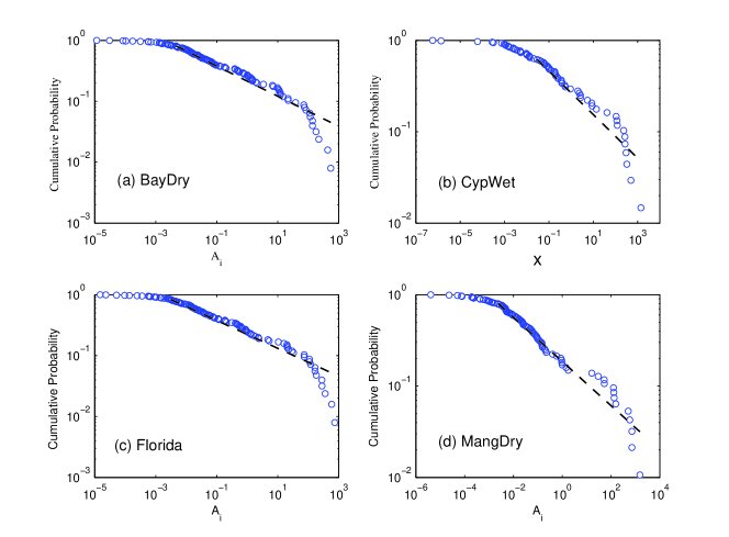
Figure 1: Cumulative probability of the variable $A_{i}$ for four selected food webs with the best fitted lines. The fitted lines start from $x_{0}$, and their slopes are listed in Table 2

$A_{i}$s of real food webs decay as power law in the high tail; therefore, the fitted lines start from given lower bounds $x_{0}$ (Clauset et al., 2007). These figures show that $A_{i}$ follows the power law distribution.

There are obvious cutoffs in the tails that may be attributed to sampling effects(Newman, 2005). According to equation 6, the cumulative probability decays as $x$ slowly. The probability of finding a higher $A_{i}$ value (in the tail of the curve) is very small. Therefore, the number of samples in this interval becomes very few and statistical fluctuations are unavoidably large as a fraction of sample number. This phenomenon is obvious in other fields such as income(Clementi et al., 2006), personal donations(Chen et al., 2009) and the number of species per genus of mammals(Newman, 2005).

The scaling exponent $\alpha$ for each food web was estimated according to the maximum likelihood approach (Clauset et al., 2007). The exponents and relative errors of power law fittings for all 21 food webs are listed in Table 2.

Table 2: Parameters of the power law distributions for $A_{i}$

($\alpha$ is the power law distribution exponent of equation 6; $x_{0}$ is the smallest value of $A_{i}$ that follows power law, $x_{max}$ is the largest $A_{i}$; $D$ is the KS statistic; $\sigma$ is the quantile of 95% confidence interval; and the number of samples is the total number of nodes following the power law distribution. The webs are sorted by their number of edges) Food web $\alpha$ $x_{0}/x_{max}$ $D$ $\sigma$ No. of samples Baydry 1.25 8.45e-006 0.09 0.13 102 Baywet 1.23 4.24e-006 0.08 0.13 105 Florida 1.23 4.24e-006 0.08 0.13 105 Mangdry 1.24 1.55e-006 0.06 0.16 75 Everglades 1.23 4.20e-006 0.12 0.20 44 Gramdry 1.25 9.55e-006 0.11 0.21 41 Gramwet 1.23 4.20e-006 0.12 0.20 44 Cypdry 1.28 5.95e-005 0.10 0.20 44 Cypwet 1.23 2.06e-005 0.10 0.21 42 Mondego 1.33 3.87e-004 0.11 0.26 26 StMarks 1.35 9.36e-004 0.17 0.21 43 Michigan 1.32 1.80e-003 0.18 0.31 18 Narragan 1.26 1.10e-004 0.16 0.23 33 ChesUpper 1.28 9.54e-004 0.21 0.23 32 ChesMiddle 1.29 9.47e-004 0.17 0.24 30 Chesapeake 1.41 8.25e-003 0.22 0.29 21 ChesLower 1.77 5.79e-002 0.20 0.33 16 CrystalC 1.27 1.04e-004 0.13 0.32 17 CrystalD 1.25 3.10e-005 0.12 0.30 19 Maspalomas 1.54 2.22e-002 0.18 0.29 20 Rhode 1.56 1.35e-002 0.17 0.34 15

In Table 2, $x_{0}$s represent the lower bounds of the power law distributions. We normalized $x_{0}$ by dividing the maximum $A_{i}$ of each food web to avoid the large range variance of $x_{0}$ among different webs because their units and the measurement time scales are very different.

$D$ is the statistic of the KS test(Rousseau and Rousseau, 2000; Goldstein et al., 2004). Its value reflects the maximum distance between the cumulative probability of real data and the fitted model. Therefore, the smaller $D$ values indicate the better power law fitting. $\sigma$ is the quantile of the 95% confidence interval for different numbers of samples(Noether, 1967), and is only a reference for $D$. If $D$ is smaller than $\sigma$, then we should accept the power-law hypothesis(Noether, 1967). From Table 2, we know that all food webs pass the KS test. In the last column, ”No. of samples” means the number of sample points that are larger than $x_{0}$ and follow the power law distribution.

By comparing different rows, we know that the food webs with more edges can be better described by power laws because their $D$s are smaller. Further, the scaling exponent $\alpha$ and $x_{0}/x_{min}$ increase as the scale of the network decreases. All $\alpha$ values fall into the interval $[1.23,1.77]$, with an average of $1.32$.

The power law distributions of $A_{i}$s reflect the heterogeneities of energy flux. Few nodes possess high $A_{i}$ values, while most nodes only share a small fraction of the energy flux. The exponent of power law reflects the degree of heterogeneity of the whole network. Therefore, larger food webs are more heterogeneous than smaller ones because their exponents are lower (Table 2). Although the power law distribution of $A_{i}$ can not give us concrete information about each vertex (Fath and Patten, 1999; Patten, 1981, 1982), it helps us to understand the network as a whole.

3.3 Power Law Distributions of $C_{i}$

The same approach can be applied to $C_{i}$s. The distributions of $C_{i}$s for four selected food webs are shown in Figure 2.

Figure 2: Cumulative probability of the variable $C_{i}$s for four selected food webs with the best fitted lines. The slopes of the fitted lines are listed in Table 3

The curves of $C_{i}$ distributions are very similar to the curves in Figure 1. The estimated exponents and the KS test parameters are listed in Table 3.

Table 3: Parameters of the power law distributions for $C_{i}$

($\beta$ is the power law distribution exponent of equation 7; $y_{0}$ is the smallest value of $C_{i}$ that follows the power law, $y_{max}$ is the largest $C_{i}$; $D$ is the KS statistic; $\sigma$ is the quantile of 95% confidence interval; the number of samples is the total number of nodes following the power law distribution. The webs are sorted by their number of edges) Food web $\beta$ $y_{0}/y_{max}$ $D$ $\sigma$ No. of samples Baydry 1.23 2.97e-006 0.08 0.13 107 Baywet 1.23 2.71e-006 0.08 0.14 101 Florida 1.23 2.71e-006 0.08 0.14 101 Mangdry 1.25 2.03e-006 0.07 0.16 68 Everglades 1.23 2.16e-006 0.10 0.20 44 Gramdry 1.25 4.57e-006 0.10 0.21 42 Gramwet 1.23 2.16e-006 0.10 0.20 44 Cypdry 1.28 4.88e-005 0.10 0.20 44 Cypwet 1.25 3.13e-005 0.11 0.21 39 Mondego 1.29 9.61e-005 0.12 0.24 30 StMarks 1.42 1.27e-003 0.16 0.21 40 Michigan 1.30 7.22e-004 0.17 0.31 18 Narragan 1.24 1.22e-004 0.17 0.23 33 ChesUpper 1.28 6.03e-004 0.20 0.23 32 ChesMiddle 1.26 3.88e-004 0.19 0.24 30 Chesapeake 1.61 2.41e-002 0.18 0.33 16 ChesLower 1.84 5.02e-002 0.22 0.35 14 CrystalC 1.28 1.04e-004 0.13 0.32 17 CrystalD 1.23 1.35e-005 0.12 0.29 20 Maspalomas 1.56 1.63e-002 0.19 0.29 20 Rhode 1.52 8.93e-003 0.23 0.32 17

Comparing Table 3 with Table 2, the exponents of $C_{i}$ distributions are slightly higher than those of $A_{i}$ distributions. The exponent $\beta$ and KS test statistic $D$ decrease with the scale of the network. The average exponent of these food webs is $1.33$, with all $C_{i}$ values falling into the interval $[1.23,1.84]$.

We have studied the heterogeneity of $C_{i}$s node by node. The nodes with high $A_{i}$ values always have high $C_{i}$ values, indicating a possible positive correlation between $A_{i}$ and $C_{i}$.

3.4 Allometric Scaling Relations

The similarity between Figure 2 and Figure 1 shows that there must be some connections between $A_{i}$ and $C_{i}$. Allometric scaling of these flow networks revealed that the relationship between $A_{i}$ and $C_{i}$ is actually a power law.

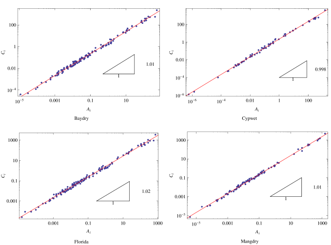
Figure 3: Allometric Scaling relationship between $A_{i}$s and $C_{i}$s of four selected food webs with the best fitted lines

As shown in Figure 3, the sample points aggregate around their fitted lines very well. This relationship is ubiquitous for all 21 food webs as shown in Table 4.

Table 4: Allometric scaling of Empirical Food Webs

(The second column lists $\eta$s of each food web with the errors; The webs are sorted by their number of edges)
Food web $\eta$ $R^{2}$ Baydry 1.01$\pm$0.01 0.9946 Baywet 1.02$\pm$0.01 0.9946 Florida 1.02$\pm$0.01 0.9946 Mangdry 1.01$\pm$0.01 0.9967 Everglades 1.02$\pm$0.01 0.9992 Gramdry 1.03$\pm$0.01 0.9990 Gramwet 1.02$\pm$0.01 0.9992 Cypdry 1.00$\pm$0.02 0.9957 Cypwet 1.00$\pm$0.01 0.9970 Mondego 1.01$\pm$0.01 0.9989 StMarks 1.03$\pm$0.04 0.9784 Michigan 1.01$\pm$0.01 0.9986 Narragan 1.01$\pm$0.04 0.9910 ChesUpper 1.05$\pm$0.02 0.9966 ChesMiddle 1.04$\pm$0.02 0.9959 Chesapeake 0.99$\pm$0.02 0.9966 ChesLower 1.05$\pm$0.02 0.9974 CrystalC 0.89$\pm$0.23 0.7706 CrystalD 0.90$\pm$0.23 0.7722 Maspalomas 0.96$\pm$0.09 0.9656 Rhode 0.83$\pm$0.17 0.8658

We used the minimum square error method to find the best-fitted line (Table 4). $R^{2}$s were larger than $0.9$ for all food webs except CrystalC, CrystalD and Rhode, whose scales are very small ($|N|<23$). The $R^{2}$s and exponents decrease with the scale of the network because the statistical significance decreases as the number of samples declines. All exponents $\eta$ fall into the interval $[0.83,1.05]$. The mean value of $\eta$s for these food webs, except CrystalC,CrystalD and Rhode, is $1.02$.

We also show the $A_{i}$ and $C_{i}$ values of root nodes for all food webs, and fit them with a line on the log-log plot (Figure 4). These power law relations reflect the self-similar nature of the weighted food webs.

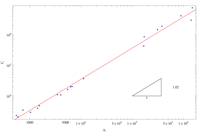
Figure 4: $A_{i}$, $C_{i}$ plot for root nodes of 21 food webs. The slope $\eta$ (the power law exponent) is 1.02$\pm$0.02

3.5 Relationship of Scaling Exponents

As we have shown, $A_{i}$ and $C_{i}$ are random variables following power law distributions with scaling exponents $\alpha$ and $\beta$, respectively. They also follow a power law relationship with the scaling exponent $\eta$. Is there any universal relationship among $\alpha,\beta$ and $\eta$?

Actually, for any random variables following power law distributions and power law relations, we can prove a mathematical theorem (see C). According to this theorem, the power law exponents $\alpha,\beta,\eta$ of the food webs should also satisfy equation 11. We tested this hypothesis by calculating $(\alpha-1)/(\beta-1)-\eta$ for each of the 21 empirical food webs to obtain Figure 5.

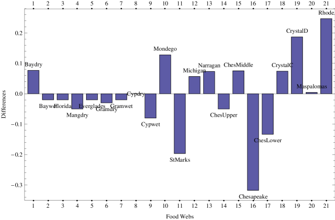
Figure 5: The differences between $\eta$ and ${(\alpha-1)}/{(\beta-1)}$ are calculated for all food webs to test the exponents relationship (equation 11). The food webs are sorted according to their number of edges

From Figure 5, we know that most exponents of food webs satisfy this relation, and that the errors become larger as the scale of the network decreases. As the scaling behaviors we are studying are statistical properties, the significance of these regularities will increase with the number of samples. Therefore, scaling behaviors are more obvious and accurate for large scale networks because larger webs have more sample points.

4 Discussion

4.1 Ecological Meaning of Power Law Exponents

As demonstrated above, food webs as energy transportation networks always follow power law distributions and relations. Three important exponents ($\alpha$,$\beta$ and $\eta$) are derived from these power law regularities. The question of whether these exponents carry ecological meaning naturally follows, and at first, the three exponents all reflect integral properties of whole networks. $\alpha$ describes the heterogeneity of first passage energy flux distributions among vertices. The heterogeneity decreases with $\alpha$. Therefore the distributions of energy flows are more uneven in large food webs than the small ones. From table 2, we also know that all $\alpha$ values fall into the interval $[1.23,1.77]$. According to the features of power law distributions, the means and variances of power law random variables with exponents smaller than 2 are divergent(Newman, 2005). Therefore, energy flux on food webs has no characteristic value. It is meaningless to find a specific species with the average energy flux as the representation of other species(Newman, 2005).

The allometric scaling relation describes the self-similarity of flow networks. Garlaschelli et al. (2003); Allesina and Bodini (2005) pointed out that allometric scaling exponents describe the transportation efficiency of binary food webs because $C_{i}$ is treated as the cost of transportation. The range of these exponents is between 1 (most inefficient network) and 2 (most efficient network). However, we believe that the exponent $\eta$ discussed in this paper does not describe the efficiency of the whole network. As pointed out in section 2 and A, $C_{i}$ can be understood as the energy store by the system, rooted from $i$ but not the cost of the transportation. Thus, the food web with higher $\eta$ can store more energy with the same consumption of metabolites ($A_{i}$). Therefore, we believe that the food webs with higher $\eta$ are more capable of storing energy by means of cycling the flows in the network. In Table 4, we see that the networks with larger scales have larger $\eta$ values. Consequently, food webs can increase their ability to store energy by increasing their complexity.

Further, the range of exponents $\eta$ is not simply $[1,2]$ (see Table 4). As Garlaschelli et al. (2003); Allesina and Bodini (2005); Banavar et al. (1999) pointed out, the range $[1,2]$ is only suitable for spanning trees or directed acyclic graphs of the original binary food webs. However, our method considers more ingredients, including the energy flux as the weight of edges, the loop structures of energy flows, and the heterogenous energy dissipation of each node, than the mere topology of the food webs with homogenous nodes. That is the reason why the exponents are out of the range $[1,2]$.

The exponent $\beta$ also describes the heterogeneity of indirect effects. It is determined by exponents $\alpha$ and $\beta$ via the theorem mentioned in section 3.5.

4.2 Flux Matrices and Fundamental Matrices

As discussed in section 2, $A_{i}$ and $C_{i}$ are defined according to the flux matrix and fundamental matrix. Therefore, the scaling behaviors of the food webs are determined by the matrices. The properties of these matrices may help us to understand the origin of the scaling behaviors.

The elements in flux matrices also follow power law distributions, with an average exponent 1.46 (see Table 5). We hypothesis that this power law determines the power law distribution of $A_{i}$.

Table 5: Parameters of the power law distributions for $f_{ij}$

($\alpha$ is the power law distribution exponent; $F_{0}$ is the smallest value of $f_{ij}$ that follows the power law; $F_{max}$ is the largest $f_{ij}$; $D$ is the KS statistic; $\sigma$ is the quantile of 95% confidence interval; number of samples is the total number of edges following the power law distribution. The webs are sorted by their number of edges)

Food web	$\alpha$	$F_{0}/F_{max}$	$D$	$\sigma$	No. of Samples
Baydry	1.33	3.82e-006	0.03	0.05	761
Baywet	1.33	4.91e-006	0.02	0.06	608
Florida	1.33	4.91e-006	0.02	0.06	608
Mangdry	1.32	2.81e-007	0.04	0.05	614
Everglades	1.37	2.98e-006	0.06	0.09	222
Gramdry	1.39	3.32e-006	0.06	0.10	194
Gramwet	1.37	2.98e-006	0.06	0.09	222
Cypdry	1.34	5.93e-005	0.05	0.10	203
Cypwet	1.29	1.15e-005	0.06	0.09	240
Mondego	1.40	4.80e-005	0.05	0.12	123
StMarks	1.84	1.29e-002	0.10	0.19	53
Michigan	1.43	5.88e-004	0.11	0.17	62
Narragan	1.70	1.43e-002	0.09	0.23	34
ChesUpper	1.32	1.95e-004	0.09	0.11	151
ChesMiddle	1.31	1.28e-004	0.11	0.12	134
Chesapeake	1.64	2.05e-002	0.17	0.24	30
ChesLower	1.65	1.17e-002	0.16	0.18	55
CrystalC	1.37	1.01e-004	0.08	0.24	30
CrystalD	1.29	6.56e-005	0.09	0.27	24
Maspalomas	1.71	2.10e-002	0.13	0.19	53
Rhode	1.84	2.65e-002	0.13	0.29	20

However, unlike other variables, the distributions of fundamental matrices are not power laws but rather more like log-normal because the tails of the curves decline quickly (see Figure 6). We also studied all of the fundamental matrices of 21 empirical food webs, and noted that very few could pass the KS test.

We presume that the calculation of the fundamental matrix in equation 3 needs infinite operations on $F$ matrix (see section 2). As a result, the noise in $F$ matrices is enlarged and accumulated in the tails of the distribution curves of $U$ matrix. However, the means by which the non-power law distribution of fundamental matrices determines power law distributions of $C_{i}$ and the allometric scaling power law relationship is an interesting problem for future studies.

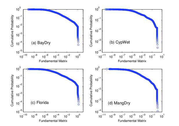
Figure 6: Cumulative distribution of fundamental matrices of four selected food webs

4.3 Information on Nodes

One of the weak points of our study on allometric scaling power law relationships is that the exponents are very close to 1. However, in this case, ”allometry” just means the non-linear relationship between two variables, so, the relationship between $A_{i}$ and $C_{i}$ cannot be rigorously defined as an allometric scaling relationship. Because the calculations of fundamental matrices and $C_{i}$s are always based on linear algebra, the results are close to linear relationship. One possible way to mend this weak point is to further consider the information available about nodes.

Indeed, much information on nodes, i.e., each species in the web, is ignored in this work. The biomass as the weight of each node is available for many food webs. According to the definition, $C_{i}$ is simply the energy store of the sub-system rooted from the vertex $i$. Therefore, biomass information should be included in $C_{i}$ because a large part of energy will flow into the species node stored as biomass. It is possible that a new approach of calculating $C_{i}$ including the biomass information for all species may break the linear relationship between $A_{i}$ and $C_{i}$.

Another important node characteristic is the body size of a given species. The metabolic theory predicts that species body size of the species can not only determine metabolism, life span, and birth rate, etc. (Brown, 2004), but also play an important role in energy flows and food webs (Cohen et al., 2003). An integrated theory of weighted food webs based on energy flow networks should contain body size data.

5 Concluding Remarks

This paper presents a new approach to reveal the scaling natures of weighted food webs as energy flow networks based on flux and fundamental matrices. The $A_{i}$,$C_{i}$ distributions and the relationship between them always follow power laws. The power law exponents $\alpha$,$\beta$ and $\eta$ satisfy a relationship, $\eta=(\alpha-1)/(\beta-1)$ as proved by the theorem 1. Power law exponents consistently change with network scales.

We note that the allometric scaling exponent does not reflect the transportation efficiency of networks but rather the capability of storing energy, which is very different from previous studies. We also investigated the distributions of flux matrices and fundamental matrices, and suggested that biomass information should be incorporated into future studies.

Acknowledgement

Thanks for the support of National Natural Science Foundation of China(No.70601002 and No.70771011). We acknowledge Clauset, A. for providing the source code of power law fitting and KS test on his web site; and also the Pajek web site to provide food web data online. We also acknowledge three anonymous reviewers for advices.

Appendix A A Simple Example

To understand the method introduced in the section 2, let’s look at a simple example (Figure 7).

Figure 7: An example to illustrate our method on deriving $A_{i}$s and $C_{i}$s

(a) is the original flow network; (b) is the balanced network from (a), the dashed arrows are artificial edges pointing to the sink node; (c) is the Markov chain calculated according to (b).

As shown in Figure 7, the balanced flow network and the derived matrix $M$ can be obtained step by step according to the method described in section 2. The fundamental matrix $U$ can then be calculated for this simple network.

$$U=I+M+M^{2}+\cdots=\left(\begin{array}[]{ccccc}1&3/5&7/20&1/5&2/5\\ 0&42/41&7/82&14/41&28/41\\ 0&12/41&42/41&4/41&8/41\\ 0&3/164&21/328&165/164&21/41\\ 0&3/82&21/164&1/82&42/41\end{array}\right)$$ (9)

Any entry $m_{ij}$ in the matrix $M$ is merely the probability of one particle flowing from vertex $i$ to vertex $j$(Barber, 1978). Furthermore, any entry $(i,j)$ in $M\cdot M$ represents the probability of a particle flowing from $i$ to $j$ along any path in $2$ steps. $M\cdot M\cdot M$ represents the probabilities after $3$ steps, etc. (Higashi et al., 1993). Thus, the matrix $U$ simply takes in consideration all transfers of particles along all possible paths.

Now, we will show how to calculate $A_{i}$ and $C_{i}$ for vertex 2. According to the definition, $A_{i}$ is the total flow-through of vertex $i$, so $A_{2}=\sum_{j=1}^{6}{f_{2,j}}=60$.

Suppose many particles are flowing in the network. They will be colored red once they flow through vertex $2$. These particles will keep their color and flow around the whole network along all possible pathways. Hence, the total number of red particles in the network is just $C_{2}$, which is computed as,

$$C_{2}=G_{2}\sum_{k=1}^{5}{u_{2k}}=((100\times 3/5+0)/(42/41))\sum_{k=1}^{5}{u_{2k}}=125$$ (10)

where the term $G_{2}=\sum_{j=1}^{5}{f_{0j}{u_{j2}}/{u_{22}}}$ in equation 10 is the total number of new particles which are colored red by vertex 2 in each time step. $\sum_{j=1}^{N}{f_{0j}{u_{j2}}}$ is the number of particles that flow into the system from the environment $0$ to the vertex $i$ along all possible pathways at each time step, with $f_{0j}=(100,0,0,0,0)$ in this example. By dividing by the term $u_{ii}$ to derive $G_{i}$ one avoids double counting the red particles(Higashi et al., 1993). Thus, $C_{i}=G_{i}\sum_{k=1}^{N}{u_{ik}}$ is the total number of particles that have been colored red and flow to other nodes along all possible pathways at each time step.

If we treat the red particles flowing in the network as a metabolic sub-system, we can calculate its allometric scaling relationship as Garlaschelli has done for binary food webs (Garlaschelli et al., 2003). Thus, $A_{i}$ is the metabolism and $C_{i}$ is the energy store or body mass of the sub-system. Indeed, Garlaschelli’s approach can be recovered by our method, as shown in the next section.

Appendix B Comparisons to Existing Approaches

In this section, we will compare our approach to Garlaschelli et al. (2003)’s method and Allesina and Bodini (2005)’s method.

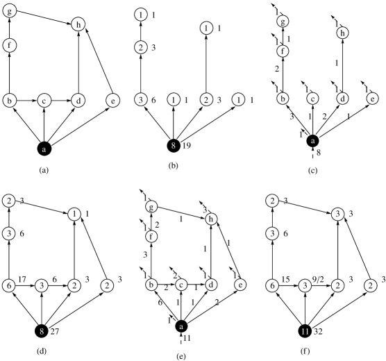
Figure 8: Calculations of allometric scaling of a hypothetical food web by various methods.

(a) is a hypothetical food web (The letter in each vertex is its index). The black vertex is the root; (b) is a spanning tree of the original network (a). $A_{i}$ and $C_{i}$ are denoted inside and beside vertex $i$; (c) is the implicated flow network of (b), the numbers beside edges are flux. The dashed lines are additional edges; (d) is a directed acyclic graph of the original network, the numbers are $A_{i}$s and $C_{i}$s calculated by the method of (Allesina and Bodini, 2005); (e) is a constructed flow network according to (d); (f) is the network with numbers of $A_{i}$s and $C_{i}$s calculated by our method according to the flow structure of (e).

Figure 8(a),(b) shows how Garlaschelli’s approach can be applied to a hypothetical food web to calculate $A_{i}$ and $C_{i}$ for each vertex. At first, a spanning tree is constructed from the original food web (Figure 8 (a)) by cutting edges. That way, each sub-tree rooted from any vertex can be viewed as a sub-system of the spanning tree. For example, the sub-tree with three vertices (b,f,g) rooted from the vertex b is a sub-system of the spanning tree. $A_{i}$ is the total number of vertices involved in this sub-tree and $C_{i}$ is the summation of $A_{i}$s for each vertex in this sub-tree. Therefore, in this example, $A_{b}$ is 3 and $C_{b}$ is 6. Finally, the universal allometric scaling relationship of $A_{i}$s and $C_{i}$s, with an exponent around $1.3$, was found for all food webs, according to Garlaschelli et al. (2003).

Garlaschelli’s method was inspired by Banavar et al. (1999)’s model to explain the Kleiber’s law (See Figure 8(c)). The spanning tree is simply Banavar’s optimal transportation network. Thus, energy flows into the whole system from the root along the links of the network to all nodes. Suppose that each node would consume 1 unit of energy in each time step. A flux with 1 unit representing the energy consumption by each node should then be added to the original spanning tree. In Figure 8(c), the energy dissipation by each node is added as a dotted line. As a result, $A_{i}$ of each node is just the total influx of this node. $C_{i}$ is the total flux (the total number of red particles colored by $i$) of the sub-tree rooted from $i$. Essentially, calculation of allometric scalings using Garlaschelli’s approach is based on this weighted flow network model. Therefore, our algorithm can derive the exact same values of $A_{i}$ and $C_{i}$ for the flow network (Figure 8(c)).

Allesina and Bodini (2005) extended Garlaschelli’s method. First, the original network is converted to a directed acyclic graph (DAG) as shown in Figure 8(d), then the sub-network originated from vertex $i$ is identified as the set of vertices that have at least one path from $i$. Therefore, vertices b,c,d,f,g,h belong to the sub-network rooted from b because they are all connected with b. $A_{i}$ is the number of vertices in the sub-network, and $C_{i}$ is the summation of all $A_{i}$s in this sub-network as shown in Figure 8(d). Because Allesina and Bodini’s approach is not based on weighted flows, it cannot be covered by our approach.

However, we can construct a balanced flow network according to the original network as shown in Figure 8(e). The information of edges is added. Our approach can be applied to this flow network to calculate $A_{i}$ and $C_{i}$ values (Figure 8(f)). Comparing Figure 8(d) to (f), we find their $A_{i}$s are almost the same, except vertices a and h. To balance the network, more flows are added in vertex h and a, so their $A_{i}$ values are larger than those in Figure 8(d). This modification can not only influence $A_{i}$ values but also $C_{i}$s. The vertices in networks 8(d) and (f) therefore have different $C_{i}$ values.

Although our approach requires weight information, it can be extended to more general flow networks, even those with cycles and loops. Also, as demonstrated by our approach, $C_{i}$ merely means the energy stored in the sub-system rooted from vertex $i$, which provides much clearer and more significant ecological meaning than previous works.

Appendix C A Theorem about Power Law Exponents

Theorem 1.

Suppose $X$ and $Y$ are two random variables following power law distributions. Their density functions, $p(x)\thicksim x^{-\alpha}$ and $p(y)\thicksim y^{-\beta}$ hold for any positive $x>x_{0},y>y_{0}$, where $x_{0}$ and $y_{0}$ are lower bounds of $X$ and $Y$. Additionally, $X$ and $Y$ satisfy a power law relation, $Y\thicksim X^{\eta}$, then the exponents $\alpha,\beta,\eta$ have following relationship:

$$\eta={{(\alpha-1)}/{(\beta-1)}}$$ (11)

Proof.

Because $X$ and $Y$ follow power law distributions, $p(x)=cx^{-\alpha}$, where $c$ is a constant that satisfies the normalization condition. And $Y=kX^{\eta}$, where $k$ is a constant, so, for any $y>kx_{0}^{\eta}$,

$$P\{Y>y\}=P\{kX^{\eta}>y\}=P\{X>({y/k})^{1/\eta}\}=\int_{({y/k})^{1/\eta}}^{+\infty}cx^{-\alpha}dx$$ (12)

Let $t=kx^{\eta}$, so $x=(t/k)^{1/\eta}$, $dx={(1/\eta)}k^{-1/\eta}t^{(1/\eta)-1}dt$. Take it into equation 12,

$$P\{Y>y\}=\int_{y}^{+\infty}(ck^{(\alpha-1)/\eta}/\eta)t^{{(1-\alpha)/\eta}-1}dt=\int_{y}^{+\infty}k^{\prime}t^{{(1-\alpha)/\eta}-1}dt$$ (13)

where $k^{\prime}=ck^{(\alpha-1)/\eta}/\eta$ is a constant. Because $Y$ follows power law distribution,

$$P\{Y>y\}=\int_{y}^{+\infty}c^{\prime}y^{-\beta}dy$$ (14)

Compare equation 13 with equation 14, we know that,

$$-\beta={(1-\alpha)/\eta}-1$$ (15)

Finally,

$$\eta={(\alpha-1)/(\beta-1)}$$ (16)

∎

References

- Albert and Barabasi (2002) Albert, R., Barabasi, A., 2002. Statistical mechanics of complex networks. Rev. Mod. Phy. 74, 47–97.