Doubly Quantized Vortices in Bulk Ginzburg-Landau Superconductors

Abstract

We have extended Brandt’s method for accurate, efficient calculations within Ginzburg-Landau theory for periodic vortex lattices at arbitrary mean induction to lattices of “doubly quantized” vortices.

I Introduction

In bulk type-II superconductors, mixed states in which the vortices carry more than one flux quantum are unstable with respect to the usual vortices that carry a single flux quantum. Near the upper critical field this result was established by Abrikosov,Abrikosov (1957) while near the lower critical field it is implied by Matricon’sMatricon (1966) calculations for isolated vortices. As far as we are aware there have been no explicit calculations within Ginzburg-Landau (GL) theory for lattices of multiply quantized vortices at magnetic field values between these two limits; but since there is no reason to believe that such lattices should be stable at intermediate fields there has been no reason to carry out the calculations.

Our motivation for doing so comes from considering thin films of type-I superconductors. In a sufficiently weak perpendicular field the magnetic flux penetrates the sample in vortices rather than intermediate state structures, and in some circumstances multiply quantized vortices are present in Ginzburg-Landau theory calculationsLasher (1967); Callaway (1992) and experiments.Hasegawa et al. (1991) We have been interestedSweeney and Gelfand (2010) in working out the phase diagram for thin films of type-I GL superconductors in arbitrary magnetic field, following Brandt’s approachBrandt (1972, 1997) to accurate and efficient solutions of the GL equations. This approach involves iterative solutions of equations, and good initial values are essential because convergence is not guaranteed. It turns out that a solution of the GL equations in bulk can be used as starting point for the film problem—this is the case even for type-I superconductors, where the bulk vortex lattice solutions are unstable with respect to the normal state. Hence, calculations for lattices of multiply quantized vortices in bulk superconductors are almost a prerequisite for the more physically motivated calculations in films.

For brevity, in this paper “singles” and “doubles” are synonymous with lattices of singly and doubly quantized vortices (carrying one and two flux quanta, respectively).

The formal developments we present are an extension of Brandt’s work in Ref. Brandt, 1997. In Sec. II we describe how Brandt’s Ansatz and iteration scheme for singles are modified for doubles. In Sec. III we offer illustrative results for order parameter and magnetic induction profiles, as well as the Gibbs free energy, for doubles and singles in a type-II superconductor. In the Appendix we discuss the solutions of the linearized GL equations, which serve as initial values for the iterative calculations.

II Formalism and Implementation

II.1 Form of solutions for doubles

Consider a vortex in which the phase of the order parameter changes by $2\pi p$ on circling the vortex core. If that core is at the origin, then the order parameter behaves as $\psi\sim r^{p}e^{ip\theta}$ as $r\to 0$ (see for example TinkhamTinkham (1996) Sec. 5.1 ) and the modulus squared order parameter as $\omega\equiv\left|\psi\right|^{2}\sim r^{2p}$. In this paper we focus on the $p=2$ case. Brandt suggestsBrandt (1997) that for a lattice with one vortex per primitive cell we adopt the Ansatz

$$\omega\left(\mathbf{r}\right)=\sum_{\mathbf{K}}a_{\mathbf{K}}\left[1-\cos\left(\mathbf{K}\cdot\mathbf{r}\right)\right]^{2}$$ (1)

in which $\mathbf{r}$ is a two-dimensional vector and $\mathbf{K}$ runs over reciprocal lattice vectors excluding the origin (as will be the case for all sums over $\mathbf{K}$ henceforth). This form satisfies the requirements of periodicity and fourth-power behavior near vortex cores. It turns out to be useful to express this with only first powers of cosines,

$$\omega\left(\mathbf{r}\right)=\sum_{\mathbf{K}}a_{\mathbf{K}}\left[\frac{3}{2}-2\cos\left(\mathbf{K}\cdot\mathbf{r}\right)+\frac{1}{2}\cos\left(2\mathbf{K}\cdot\mathbf{r}\right)\right]$$ (2)

In a bulk superconductor $\mathbf{B}\left(\mathbf{r}\right)=B\left(\mathbf{r}\right)\mathbf{\hat{z}}$. For small $r$ the induction satisfies $B\left(\mathbf{r}\right)\approx B\left(0\right)-\frac{1}{2\kappa}\omega\left(\mathbf{r}\right)$, so $B\left(0\right)-B\left(r\right)\sim r^{4}$. The small-$r$ behavior suggests the following form for the deviation from mean induction, $b\left(\mathbf{r}\right)=B\left(\mathbf{r}\right)-\bar{B}$,

$$b\left(\mathbf{r}\right)=\sum_{\mathbf{K}}b_{\mathbf{K}}\left[2\cos\left(\mathbf{K}\cdot\mathbf{r}\right)-\frac{1}{2}\cos\left(2\mathbf{K}\cdot\mathbf{r}\right)\right]$$ (3)

The supervelocity can be decomposed as $\mathbf{Q}\left(\mathbf{r}\right)=\mathbf{Q}_{A}\left(\mathbf{r}\right)+\mathbf{q}\left(\mathbf{r}\right)$, where $\mathbf{Q}_{A}$ is the supervelocity in the Abrikosov limit, satisfying $\nabla\times\mathbf{Q}_{A}\left(\mathbf{r}\right)=\left[\bar{B}-2\Phi_{0}\delta\left(\mathbf{r}\right)\right]\mathbf{\hat{z}}$, (with $\Phi_{0}$ the flux quantum) and the deviation from the Abrikosov form has the property that $\hat{\mathbf{z}}\cdot(\nabla\times\mathbf{q}\left(\mathbf{r}\right))=b\left(\mathbf{r}\right)$. This last relation implies

$$\mathbf{q}\left(\mathbf{r}\right)=\sum_{\mathbf{K}}b_{\mathbf{K}}\frac{\mathbf{\hat{z}}\mathbf{\times K}}{\left|\mathbf{K}^{2}\right|}\left[2\sin\left(\mathbf{K}\cdot\mathbf{r}\right)-\frac{1}{4}\sin\left(2\mathbf{K}\cdot\mathbf{r}\right)\right]$$ (4)

The mean induction $\bar{B}$ fixes the area $S$ of the lattice unit cell, through $S=2\Phi_{0}/\bar{B}$. The unit cell has primitive lattice vectors $\mathbf{R}_{10}=x_{1}\hat{\mathbf{x}}$, $\mathbf{R}_{01}=x_{2}\hat{\mathbf{x}}+y_{2}\hat{\mathbf{y}}$ and in those terms $S=(\mathbf{R}_{10}\times\mathbf{R}_{01})\cdot\hat{\mathbf{z}}=x_{1}y_{2}$. The general reciprocal lattice vector is $\mathbf{K}_{mn}=2\pi\left[my_{2}\hat{\mathbf{x}}+\left(mx_{2}+nx_{1}\right)\hat{\mathbf{y}}\right]/S$.

II.2 Iterative expressions

The GL free energy per unit volume $F$, referenced from the Meissner state, may be expressed in gauge invariant form and in the standard reduced units asBrandt (1997)

$$F=\left\langle\frac{1}{2}-\omega+\frac{1}{2}\omega^{2}+\frac{\left|\nabla\omega\right|^{2}}{4\kappa^{2}\omega}+\omega\left|\mathbf{Q}\right|^{2}+\left|\mathbf{B}\right|^{2}\right\rangle$$ (5)

where angle brackets denote integration over a two-dimensional unit cell, $\left\langle\cdots\right\rangle=\frac{1}{S}\int_{S}\cdots dx\,dy$. Extremalization of $F$ yields the first GL equation

$$-\nabla^{2}\omega=2\kappa^{2}\left[\omega-\omega^{2}-\omega\left|\mathbf{Q}\right|^{2}-g\right]$$ (6)

where

$$g\equiv|\nabla\omega|^{2}/4\kappa^{2}\omega$$ (7)

and the second GL equation

$$\nabla\times B\hat{\mathbf{z}}=-\omega\mathbf{Q}$$ (8)

The first GL equation leads to an iterative equation for $a_{\mathbf{K}}$. Following Brandt, a stabilizing term $2\kappa^{2}\omega$ is added to both sides of Eq. (6) and then the equation is multiplied by $\cos\mathbf{K}\cdot\mathbf{r}$ and integrated over the unit cell. The expansion (2) is inserted for $\omega$ on the left side of the equation, and the orthogonality relation $\left\langle\cos\left(\mathbf{K}\cdot\mathbf{r}\right)\cos\left(\mathbf{K}^{\prime}\cdot\mathbf{r}\right)\right\rangle=\frac{1}{2}\delta_{\mathbf{K},\mathbf{K}^{\prime}}$ enables the integral on the left side to be done analytically. Rearranging leads to an identity which we treat as a step in an iterative solution for $a_{\mathbf{K}}$,

$$a_{\mathbf{K}}:=\frac{2\kappa^{2}}{\left|\mathbf{K}\right|^{2}+2\kappa^{2}}\langle(-2\omega+\omega^{2}+\omega\left|\mathbf{Q}\right|^{2}+g)\cos\mathbf{K}\cdot\mathbf{r}\rangle$$ (9)

$$+\frac{1}{4}a_{\mathbf{K}/2}$$

If $\mathbf{K}/2$ is not a reciprocal lattice vector then $a_{\mathbf{K}/2}\equiv 0$; we will refer to such reciprocal lattice vectors as “fundamentals.” Eq. (9) should be compared with the corresponding relation for singles, Eq. (11) in Ref. Brandt, 1997: the only differences are the existence of the second term and a factor of two in the first term.

The next step in the iterative scheme is to rescale all of the $a_{\mathbf{K}}$ so as to minimize $F$. This goes through without modification

$$a_{\mathbf{K}}:=a_{\mathbf{K}}\langle\omega-\omega\left|\mathbf{Q}\right|^{2}-g\rangle/\langle\omega^{2}\rangle$$ (10)

The iterative equation for $b_{\mathbf{K}}$ is derived in the same manner as Eq. (9). Taking the curl of Eq. (8), adding a stabilizing term $-\langle\omega\rangle B\left(\mathbf{r}\right)$ to both sides, multiplying by $\cos\mathbf{K}\cdot\mathbf{r}$, integrating over the unit cell, inserting the expansion (3) on the left hand side, applying orthogonality of cosines, and rearranging leads to

$$b_{\mathbf{K}}:=-\frac{\langle[(\omega-\langle\omega\rangle)B\left(\mathbf{r}\right)+(\nabla\omega\times\mathbf{Q})\cdot\hat{z}]\cos\mathbf{K}\cdot\mathbf{r}\rangle}{\left|\mathbf{K}\right|^{2}+\langle\omega\rangle}$$ (11)

$$+\frac{1}{4}b_{\mathbf{K}/2}$$

Again, if $\mathbf{K}$ is a fundamental then the coefficient $b_{\mathbf{K}/2}\equiv 0$.

The GL equations are solved, in principle, by cycling through Eqs. (9), (10), and (11) until the coefficients converge to the desired level of precision. In practice we find that the equations as written do not usually converge to a physical solution; however, by “mixing” the $a_{\mathbf{K}}$ that comes out of (9) with the value from the prior iteration (and likewise for the $b_{\mathbf{K}}$ produced by (11)) the convergence of the algorithm is much improved, though at the cost of more iterations. We have not attempted to determine optimal mixing parameters. Taking 90% of the prior iteration plus 10% of the current iteration is sufficient for every calculation we have carried out so far.

Even with mixing, it is crucial to have a good initial guess for the $a_{\mathbf{K}}$ and $b_{\mathbf{K}}$. Brandt has demonstratedBrandt (1997) that the solution of the linearized GL equations for the $a_{\mathbf{K}}$, together with $b_{\mathbf{K}}=0$ for all $\mathbf{K}$, serves well for the initial values for singles, and we find the same to be true for doubles. Constructing solutions to the linearized GL equations for doubles in terms of the $a_{\mathbf{K}}$ is not trivial, and we detail our method in Appendix A. The solution to the linearized GL equations is used to begin the iteration cycle in Eq. (10).

II.3 Implementation issues

In order to have a finite computational problem the expansions for $\omega$, $b$, and $\mathbf{q}$ must be truncated; and the iterations involve integrals over the unit cell which must be numerically evaluated. These two issues are related. For singles, it is sufficient to carry out the quadrature by summation of values on a grid aligned with the primitive lattice vectors, and to include in the expansions only $|\mathbf{K}|\leq K_{\mathrm{max}}$ with $K_{\mathrm{max}}$ chosen so that the number of reciprocal lattice vectors is the same as the number of points in the integration grid. For doubles the situation is more complicated.

Observe that the expansion (2) for $\omega$ can be rearranged so that it has nearly the same form as for singles,

$$\omega\left(\mathbf{r}\right)=\sum_{\mathbf{K}}\left[2a_{\mathbf{K}}-\frac{1}{2}a_{\mathbf{K}/2}\right]\left[1-\cos\left(\mathbf{K}\cdot\mathbf{r}\right)\right]$$ (12)

When $\mathbf{K}$ is a fundamental, as defined following Eq. (9), $a_{\mathbf{K}/2}\equiv 0$. Eqs. (1), (2) and (12) are identical for infinite sums, but they are different when truncated. As discussed in Appendix A, the $a_{\mathbf{K}}$ that solve the linearized GL equations for doubles do not fall off in a Gaussian manner like they do for singles; however, the $2a_{\mathbf{K}}-\frac{1}{2}a_{\mathbf{K}/2}$ are approximately Gaussian. This motivates the following truncation scheme for constructing $\omega$ when evaluating the integrals over the unit cell: use Eq. 12, including in the sum reciprocal lattice vectors with $|\mathbf{K}|\leq K_{\mathrm{max}}$ except for fundamentals with $K_{\mathrm{max}}/2<|\mathbf{K}|\leq K_{\mathrm{max}}$. Expressions analogous to Eq. 12 exist for $b$ and $\mathbf{q}$, namely

$$b\left(\mathbf{r}\right)=\sum_{\mathbf{K}}\left[2b_{\mathbf{K}}-\frac{1}{2}b_{\mathbf{K}/2}\right]\cos\left(\mathbf{K}\cdot\mathbf{r}\right)$$ (13)

$$\mathbf{q}\left(\mathbf{r}\right)=\sum_{\mathbf{K}}\left[2b_{\mathbf{K}}-\frac{1}{2}b_{\mathbf{K}/2}\right]\sin\left(\mathbf{K}\cdot\mathbf{r}\right)\frac{\mathbf{\hat{z}}\mathbf{\times K}}{\left|\mathbf{K}^{2}\right|}$$ (14)

and we apply the same truncation scheme.

We conclude this section with a warning. It is tempting to define $c_{\mathbf{K}}\equiv 2a_{\mathbf{K}}-\frac{1}{2}a_{\mathbf{K}/2}$, $d_{\mathbf{K}}\equiv 2b_{\mathbf{K}}-\frac{1}{2}b_{\mathbf{K}/2}$, and carry out iterative calculations for those quantities, by moving the $\frac{1}{4}a_{\mathbf{K}/2}$ from the right side of Eq. (9) to the left (and likewise for Eq. (11)): the resulting equations have exactly the form of Eqs. 11 and 13 from Ref. Brandt, 1997 for the iterations of the coefficients for singles. Doing this invariably leads to a “singles-like” solution ($\omega\sim r^{2}$ and $B\left(0\right)-B\left(r\right)\sim r^{2}$ for small $r$) which is inconsistent with the assumed forms of $\bar{B}$, $\mathbf{Q}_{A}$ and $S$; in addition this unphysical solution is a free energy saddle point rather than a minimum.

III Results and Conclusions

To illustrate the effectiveness of the calculational scheme described in the previous section, we will present results for $\kappa=1$ for triangular arrays of both doubly and singly quantized vortices. In comparing doubles with singles it is important to do the calculations on an equal footing; with this in mind, in order to have the same spacing between real-space grid points in both calculations we use about twice as many grid points for doubles than for singles. For $\bar{B}$ greater than $\mu_{0}H_{c2}/5$ we typically use 32 points along each primitive lattice vector for singles and 46 for doubles. Singles and doubles then have the same $K_{\mathrm{max}}$ but the doubles calculation includes twice as many reciprocal lattice vectors as the singles calculation. A typical singles calculation converges in approximately 50 iterations while the doubles require about four times as many. At lower inductions the area of the vortex core becomes considerably less than the area of the unit cell, and in order to represent the solutions well the real-space sampling needs to be refined by increasing the number of grid points per unit cell edge to 64 or 96 for singles and with proportionally increased numbers for doubles. The growth in the number of grid points and reciprocal lattice vectors puts a practical lower limit on the mean induction of $\mu_{0}H_{c2}/10$.

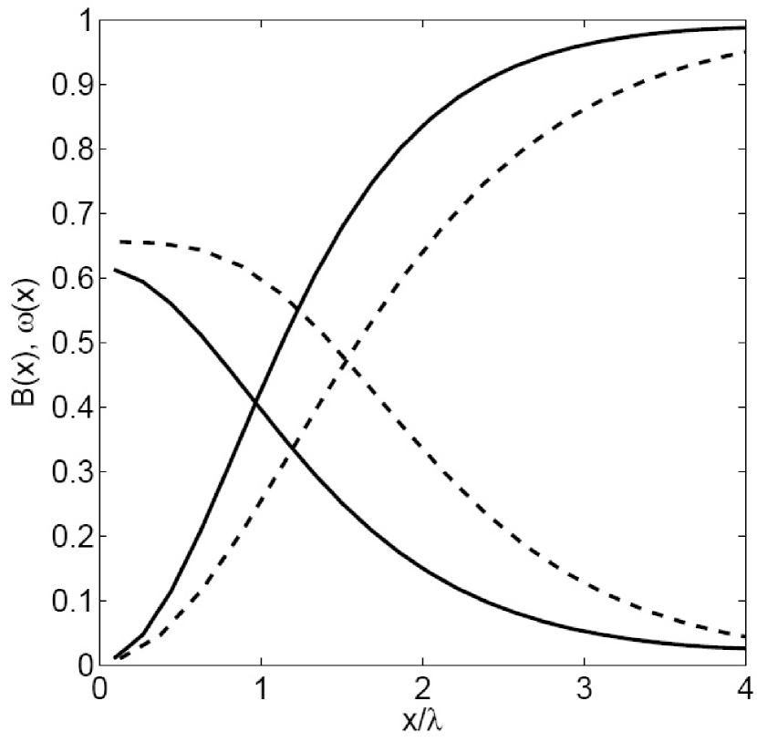
Figure 1: Cross sections along $y=0$ of induction (curves decreasing from $x=0$) and squared order parameter (curves increasing from $x=0$) for doubly quantized (dashed) and singly quantized (solid) triangular vortex lattices at the same parameters $\kappa=1$ and $\bar{B}=\mu_{0}H_{c2}/10$. The inter-vortex spacing for singles is $8.5\lambda$ and is greater by a factor of $\sqrt{2}$ for doubles.

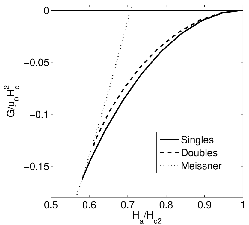
Figure 2: Gibbs free energy density, referenced from the normal state, as a function of applied field at GL parameter $\kappa=1$.

In Figure 1 we show the order parameter and induction along a line connecting two adjacent vortices at $\bar{B}=\mu_{0}H_{c2}/10$ for both doubles and singles. As one would expect, the vortex cores for doubles are wider than for singles. In Fig. 2 we present the Gibbs free energy density $G=F-\mathbf{H}_{a}\cdot\mathbf{B}$ in the full range of applied fields $H_{c1}\leq H_{a}\leq H_{c2}$ for triangular singles and doubles. The applied field $H_{a}$ is calculated in the same manner as in Refs. Klein and Pöttinger, 1991; Brandt, 1997, based on the virial theorem of Doria, Gubernatis, and Rainer.Doria et al. (1989) These results confirm that doubles are thermodynamically unstable in bulk type-II superconductors. Similar results are obtained for other values of $\kappa>1/\sqrt{2}$. The calculations also yield convergent results for type-I superconductors but in such cases all vortex states are unstable with respect to the Meissner state.

In conclusion, we have produced precise numerical solutions to the GL equations consisting of infinite lattices of “doubly quantized” vortices in bulk superconductors. The calculations can be carried out efficiently for mean inductions down to 10% of the upper critical value. Although such solutions of the GL equations never globally minimize the GL free energy for bulk superconductors, we expect they will be useful as starting points for solving the GL equations in film geometry.

Appendix A Solving the Linearized GL equations in Terms of the $a_{\mathbf{K}}$

In his pioneering work on vortex lattices in superconductors, AbrikosovAbrikosov (1957) showed that for an applied field just below $H_{c2}$, the first GL equation (when expressed as an equation for the order parameter) has the form of Schrödinger’s equation for a charged particle confined to a plane and subject to a magnetic field. With an assumed periodicity of the vortex lines and one flux quantum per vortex, an analytic solution $\psi_{A}$ exists and can be expressedAbrikosov (1957); Kleiner et al. (1964); Brandt (1969) in terms of a Jacobi theta function,

$$\psi_{A}\left(x,y\right)=e^{-\pi y^{2}/x_{1}y_{2}}\vartheta_{1}\left(\frac{\pi}{x_{1}}\left(x+iy\right),\frac{x_{2}+iy_{2}}{x_{1}}\right)$$ (15)

where $\vartheta_{1}\left(z,\tau\right)\equiv 2\sum_{n=0}^{\infty}\left(-\right)^{n}e^{i\pi\tau\left(n+\frac{1}{2}\right)^{2}}\sin(2n+1)z$ and the lattice parameters $x_{1}$, $x_{2}$ and $y_{2}$ were defined just below Eq. (4). With this form for $\psi_{A}$ its modulus squared, $\omega_{A}\equiv\left|\psi_{A}\right|^{2}$, is expressed as a double sum. This leadsBrandt (1972) to the Fourier like expansion of real terms, $\omega_{A}=\sum_{\mathbf{K}}a_{\mathbf{K}}^{A}\left[1-\cos\left(\mathbf{K}\cdot\mathbf{r}\right)\right]$, with $a_{\mathbf{K}}^{A}=-\left(-\right)^{m+mn+n}e^{-K_{mn}^{2}S/8\pi}$. Note that the sum over $\mathbf{K}$ is still a double sum over $m$ and $n$.

LasherLasher (1965) pointed out that for vortices of multiplicity $p$, $\psi_{A}^{\left(p\right)}\left(r\right)=\left[\psi_{A}\left(r/\sqrt{p}\right)\right]^{p}$ is a corresponding solution of the linearized GL equations. In principle one could use this form to determine $a_{\mathbf{K}}^{A}$ for doubles in the expansion (1), starting from (15), but we did not attempt to carry that through.

We have taken an alternative approach based on numerical solution of a linear system for the $a_{\mathbf{K}}^{A}$ derived from the linearized GL equations. In the linear regime $b\left(\mathbf{r}\right)=B(0)-\bar{B}-\omega_{A}\left(\mathbf{r}\right)/2\kappa$ (see, for example, De Gennesde Gennes (1966) Sec. 6.7). Taking the curl and combining with the second GL equation yields

$$\frac{1}{2\kappa}\nabla\omega_{A}\times\hat{\mathbf{z}}=\omega_{A}\mathbf{Q}_{A}$$ (16)

Combining (16), (2), and the Fourier expansion for the supervelocity in the Abrikosov limit (see Eq. (24) in Ref. Brandt, 1972), then applying uniqueness of Fourier series leads to the linear system

$$\sum_{\mathbf{K}_{i}}A_{ji}a_{\mathbf{K}_{i}}^{A}=-\langle\omega_{A}\rangle$$ (17)

with

$$A_{ji}\equiv C_{ji}-\delta_{\mathbf{K}_{i},\mathbf{K}_{j}}\frac{1}{2\bar{B}\mathbf{\kappa}}\left|\mathbf{K}_{j}\right|^{2}+\delta_{\mathbf{K}_{i},\mathbf{K}_{j}/2}\frac{1}{8\bar{B}\mathbf{\kappa}}\left|\mathbf{K}_{j}\right|^{2}$$ (18)

and

$$C_{ji}\equiv-\frac{\left|\mathbf{K}_{j}\right|^{2}-\mathbf{K}_{i}\cdot\mathbf{K}_{j}}{\left|\mathbf{K}_{j}-\mathbf{K}_{i}\right|^{2}}-\frac{\left|\mathbf{K}_{j}\right|^{2}+\mathbf{K}_{i}\cdot\mathbf{K}_{j}}{\left|\mathbf{K}_{j}+\mathbf{K}_{i}\right|^{2}}$$ (19)

$$+\hskip 3.0pt\frac{\left|\mathbf{K}_{j}\right|^{2}-2\mathbf{K}_{i}\cdot\mathbf{K}_{j}}{4\left|\mathbf{K}_{j}-2\mathbf{K}_{i}\right|^{2}}+\frac{\left|\mathbf{K}_{j}\right|^{2}+2\mathbf{K}_{i}\cdot\mathbf{K}_{j}}{4\left|\mathbf{K}_{j}+2\mathbf{K}_{i}\right|^{2}}$$

We follow Brandt’s convention that $\langle\omega_{A}\rangle=1$, so $(3/2)\sum_{\mathbf{K}}a_{\mathbf{K}}^{A}=1$.

The infinite system of equations (17) could be rendered finite by setting $a_{\mathbf{K}}^{A}=0$ for $|\mathbf{K}|>K_{\mathrm{max}}$; however, this is not a good closure assumption because of slow convergence with increasing $K_{\mathrm{max}}$. Eq. (18) shows the strong connection between $a_{\mathbf{K}}^{A}$ and $a_{\mathbf{K}/2}^{A}$ previously mentioned in Sec. II.3. In particular, for $K_{\mathrm{max}}/2<|\mathbf{K}|\leq K_{\mathrm{max}}$ the corresponding $a_{\mathbf{K}}^{A}$ are connected to coefficients associated with vectors beyond the cutoff. In addition, as $|\mathbf{K}_{j}|\to\infty$, $C_{ji}\to-3/2$, which leads to $a_{\mathbf{K}}^{A}\approx a_{\mathbf{K}/2}^{A}/4$ at large $|\mathbf{K}|$. (For large $|\mathbf{K}_{j}|$, $\sum_{\mathbf{K}_{i}}C_{ji}a_{\mathbf{K}_{i}}^{A}\approx-(3/2)\sum_{\mathbf{K}}a_{\mathbf{K}}^{A}=-\langle\omega_{A}\rangle$, hence the latter two terms on the right side of Eq. 18 must sum to zero.) We therefore set $a_{2\mathbf{K}}^{A}=a_{\mathbf{K}}^{A}/4$, $a_{4\mathbf{K}}^{A}=a_{\mathbf{K}}^{A}/16$, and so on for $K_{\mathrm{max}}/2<|\mathbf{K}|\leq K_{\mathrm{max}}$ and this leads to a modified linear system with coefficients $A^{\prime}_{ji}$. For $i$ such that $K_{\mathrm{max}}/2<|\mathbf{K}_{i}|\leq K_{\mathrm{max}}$,

$$A^{\prime}_{ji}=A_{ji}+\sum_{l=1}^{\infty}4^{-l}C_{j,2^{l}i}$$ (20)

with $\mathbf{K}_{2^{l}i}\equiv 2^{l}\mathbf{K}_{i}$. We truncate the sum at $l=4$ after finding no change in the results for $a_{\mathbf{K}}^{A}$ when further terms are included.

In Figs. 3 and 4 we show the results of numerically solving the linear system for $\kappa=1$ and $K_{\mathrm{max}}=36$. In the former only $a_{\mathbf{K}}^{A}$ for fundamental reciprocal lattice vectors are shown; while in the latter $a_{\mathbf{K}}^{A}$ for reciprocal lattice vectors that are powers of two times several different fundamentals are displayed, showing that $a_{\mathbf{K}}^{A}\approx a_{\mathbf{K}/2}^{A}/4$ holds even for $|\mathbf{K}|$ not very large.

Finally, let us note that as a check on this approach to solving the linearized GL equations we have carried an analogous analysis for singles. The numerical results from solving the corresponding linear equation for the $a_{\mathbf{K}}^{A}$ match the exact, analytic results.

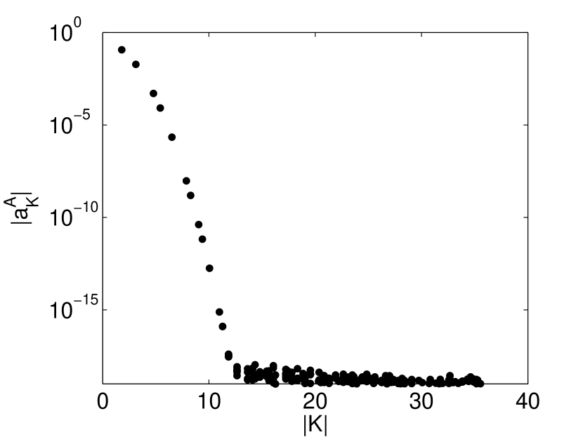
Figure 3: Solutions to the linear system for the $a_{\mathbf{K}}^{A}$ associated with fundamental reciprocal lattice vectors.

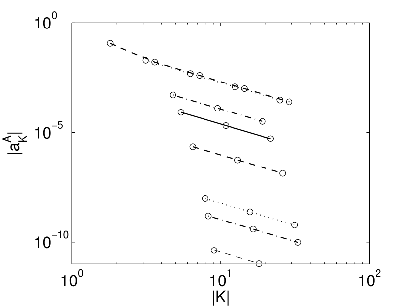
Figure 4: Solutions to the linear system for the $a_{\mathbf{K}}^{A}$ associated with eight fundamental reciprocal lattice vectors and those vectors multiplied by powers of two. The lines are guides to the eye connecting $a_{\mathbf{K}}^{A}$, $a_{2\mathbf{K}}^{A}$, $a_{4\mathbf{K}}^{A}$,…

References

- Abrikosov (1957) A. A. Abrikosov, Zh. Eksp. Teor. Fiz. 32, 1442 (1957).
- Matricon (1966) J. Matricon, Ph.D. thesis, Université de Paris (1966).
- Lasher (1967) G. Lasher, Phys. Rev. 154, 345 (1967).
- Callaway (1992) D. J. E. Callaway, Ann. Phys. (NY) 213, 166 (1992).
- Hasegawa et al. (1991) S. Hasegawa, T. Matsuda, J. Endo, N. Osakabe, M. Igarashi, T. Kobayashi, M. Naito, A. Tonomura, and R. Aoki, Phys. Rev. B 43, 7631 (1991).
- Sweeney and Gelfand (2010) M. C. Sweeney and M. P. Gelfand, arXiv:1003.0648v1 (2010).
- Brandt (1972) E. H. Brandt, Phys. Status Solidi B 51, 345 (1972).
- Brandt (1997) E. H. Brandt, Phys. Rev. Lett. 78, 2208 (1997).
- Tinkham (1996) M. Tinkham, Introduction to superconductivity (McGraw Hill, New York, 1996), 2nd ed.
- Klein and Pöttinger (1991) U. Klein and B. Pöttinger, Phys. Rev. B 44, 7704 (1991).
- Doria et al. (1989) M. M. Doria, J. E. Gubernatis, and D. Rainer, Phys. Rev. B 39, 9573 (1989).
- Kleiner et al. (1964) W. H. Kleiner, L. M. Roth, and S. H. Autler, Phys. Rev. 133, A1226 (1964).
- Brandt (1969) E. H. Brandt, Phys. Status Solidi B 36, 393 (1969).
- Lasher (1965) G. Lasher, Phys. Rev. 140, A523 (1965).
- de Gennes (1966) P. de Gennes, Superconductivity of metals and alloys (W.A. Benjamin, New York, 1966).