Controlling Chaotic Transport on Periodic Surfaces

Abstract

We uncover and characterize different chaotic transport scenarios on perfect periodic surfaces by controlling the chaotic dynamics of particles subjected to periodic external forces in the absence of a ratchet effect. After identifying relevant symmetries of chaotic solutions, analytical estimates in parameter space for the occurrence of different transport scenarios are provided and confirmed by numerical simulations. These scenarios are highly sensitive to variations of the system’s asymmetry parameters, including the eccentricity of the periodic surface and the direction of dc and ac forces, which could be useful for particle sorting purposes in those cases where chaos is unavoidable.

Introduction.$-$Controlling the transport of particles on periodic potential energy surfaces is an old and ubiquitous problem appearing in different fields such as physics, chemistry, and biology 1 . Specific examples include colloidal transport in arrays of optical tweezers 2 , flux creep through type-II superconductors 3 , and Bose-Einstein condensates with periodic pinning sites 4 , among many other. Previous theoretical analysis of the motion of particles on surfaces 5 ; 6 ; 7 ; 8 ; 9 ; 10 considered mesoscopic models owing to the great complexity of the different transport scenarios. While non-chaotic regimes have been widely studied in the context of noisy overdamped models 11 and the chaotic regime has been mainly considered when directed transport is induced by symmetry breaking 9 ; 12 , to the best of our knowledge, the fundamental case of deterministic chaotic transport in the absence of a ratchet effect has not been considered in detail as yet. The study of such a chaotic transport on simple periodic surfaces could indeed shed some light on diverse chaotic phenomena of great complexity appearing for example in magnetotransport on antidot lattices 13 .

Model.$-$In this Letter, we consider the classical dynamics of a dissipative particle moving on a standard separable periodic potential, with an external force having both dc and ac components, and neglecting thermal effects: $m\overset{..}{x}+\partial V/\partial x=-\mu\overset{.}{x}+f_{0}\cos\theta+f_{1x}\cos\left(\omega_{x}t\right)$, $m\overset{..}{y}+\partial V/\partial y=-\mu\overset{.}{y}+f_{0}\sin\theta+f_{1y}\cos\left(\omega_{y}t\right)$, where an overdot denotes a derivative with respect to $t$, $\theta$ describes the direction of the dc force $\mathbf{f}_{0}$, $\mu$ is the phenomenological coefficient of friction, and $V(x,y)=V_{0}\left[\cos\left(2\pi x/\lambda_{x}\right)+\cos\left(2\pi y/\lambda_{y}\right)\right]/2$ is the potential with $\lambda_{x},\lambda_{y}$ being the characteristic length scales. A main purpose of the present work is a theoretical characterization of the different chaotic transport (CT) scenarios by providing analytical estimates of the threshold conditions in parameter space by using Melnikov analysis (MA). For the sake of a dimensionless description, we put the equations of motion into the form

$$\overset{..}{r}_{x}+\sin r_{x} = -\gamma\overset{.}{r}_{x}+F_{0x}\cos\theta+F_{1x}\cos\left(\Omega_{x}\tau\right),$$ (1)

$$\overset{..}{r}_{y}+\frac{\sin r_{y}}{a^{2}} = -\gamma\overset{.}{r}_{y}+\frac{F_{0x}}{a}\sin\theta+\frac{F_{1x}b}{a}\cos\left(c\Omega_{x}\tau\right),$$ (2)

where all variables and parameters are dimensionless, an overdot denotes a derivative with respect to $\tau\equiv\pi t\left(2V_{0}/m\right)^{1/2}/\lambda_{x}$, $r_{x}\equiv 2\pi x/\lambda_{x}\pm\pi$, $r_{y}\equiv 2\pi y/\lambda_{y}\pm\pi$, $\gamma\equiv\mu\lambda_{x}\left(2mV_{0}\right)^{-1/2}/\pi$, $F_{0x}\equiv f_{0}\lambda_{x}/\left(\pi V_{0}\right)$, $F_{1x}\equiv\lambda_{x}f_{1x}/\left(\pi V_{0}\right)$, $\Omega_{x}\equiv\omega_{x}\lambda_{x}\left[m/\left(2V_{0}\right)\right]^{1/2}/\pi$, $a\equiv\lambda_{y}/\lambda_{x}$, $b\equiv f_{1y}/f_{1x}$, and $c\equiv\omega_{y}/\omega_{x}$. It is also assumed that the system [Eqs. (1)-(2)] satisfies the MA requirements, i.e., the dissipation and forcing terms are small-amplitude perturbations of the underlying conservative pendula $\overset{..}{r}_{x,y}+\sin r_{x,y}=0$ (see 14 ; 15 ; 16 for general background). Straightforward application of MA to Eqs. (1) and (2) yields the Melnikov functions (MFs)

$$M_{x}^{\pm}\left(\tau_{0}\right) = D_{x}^{\pm}\pm 2\pi F_{1x}\rm{sech}\left(\frac{\pi\Omega_{x}}{2}\right)\cos\left(\Omega_{x}\tau_{0}\right),$$ (3)

$$M_{y}^{\pm}\left(\tau_{0}\right) = D_{y}^{\pm}\pm 2\pi abF_{1x}\rm{sech}\left(\frac{\pi ac\Omega_{x}}{2}\right)\cos\left(c\Omega_{x}\tau_{0}\right),$$ (4)

respectively, where the positive (negative) sign refers to the top (bottom) homoclinic orbit of the conservative pendulum, and $D_{x}^{\pm}\equiv\pm 2\pi F_{0x}\cos\theta-8\gamma$, $D_{y}^{\pm}\equiv\pm 2\pi aF_{0x}\sin\theta-8a\gamma$. Since the MFs (3) and (4) have an infinity of simple zeros, a main conclusion is that necessary conditions for the onset of chaotic instabilities are, respectively,

$$F_{1x} > \frac{\min\left\{\left|D_{x}^{+}\right|,\left|D_{x}^{-}\right|\right\}}{2\pi}\cosh\left(\frac{\pi\Omega_{x}}{2}\right),$$ (5)

$$F_{1x} > \frac{\min\left\{\left|D_{y}^{+}\right|,\left|D_{y}^{-}\right|\right\}}{2\pi ab}\cosh\left(\frac{\pi ac\Omega_{x}}{2}\right).$$ (6)

Next, one can compare the theoretical predictions and Lyapunov exponent (LE) calculations 15 with the caveat that one cannot expect too good a quantitative agreement between the two kinds of results because LE provides information concerning solely steady chaos, while MM is a perturbative method generally related to transient chaos 16 . To quantify the sorting capability associated with the threshold of chaotic transport, we evaluate the Cartesian components of the velocity, $\left\langle v_{i}\right\rangle=\lim_{\tau\rightarrow\infty}\left\langle r_{i}(\tau)\right\rangle/\tau$ $\left(i=x,y\right)$, where brackets indicate average over initial conditions, and construct the velocity components parallel and perpendicular to the external dc force $\mathbf{f}_{0}$, $\left\langle v_{\|}\right\rangle=\left\langle v_{x}\right\rangle\cos\theta+a\left\langle v_{y}\right\rangle\sin\theta$, and $\left\langle v_{\bot}\right\rangle=-\left\langle v_{x}\right\rangle\sin\theta+a\left\langle v_{y}\right\rangle\cos\theta$, respectively. We characterize the deviation of $\left\langle\mathbf{v}\right\rangle$ from $\mathbf{f}_{0}$ by means of the quantifier

$$\tan\alpha=\left\langle v_{\bot}\right\rangle/\left\langle v_{\|}\right\rangle,$$ (7)

where $\alpha$ is the deflection angle 10 . For the sake of clarity, we shall consider here the case with equal frequencies $\left(c=1\right)$ and both dc and ac forces acting in the same direction ($f_{1x}\equiv f_{1}\cos\theta,f_{1y}\equiv f_{1}\sin\theta$, and hence $b=\tan\theta$). By defining $F_{1}\equiv\lambda_{x}f_{1}/\left(\pi V_{0}\right)$, one has $F_{1x}=F_{1}\cos\theta$ and hence Eqs. (5) and (6) reduce to

$$F_{1} > F_{1,th}^{x}\equiv\frac{\min\left\{\left|D_{x}^{+}\right|,\left|D_{x}^{-}\right|\right\}}{2\pi\left|\cos\theta\right|}\cosh\left(\frac{\pi\Omega_{x}}{2}\right),$$ (8)

$$F_{1} > F_{1,th}^{y}\equiv\frac{\min\left\{\left|D_{y}^{+}\right|,\left|D_{y}^{-}\right|\right\}}{2\pi a\left|\sin\theta\right|}\cosh\left(\frac{\pi a\Omega_{x}}{2}\right),$$ (9)

respectively, where $F_{1,th}^{x},F_{1,th}^{y}$ are the chaotic threshold amplitudes.

Symmetry analysis.$-$Equations (8) and (9) tell us that the onset of chaos in both directions strongly depends upon the external force direction $\theta$, which can thus be used as a high-sensitivity control parameter to suppress and strength CT in one or the another direction at will. Specifically, one straightforwardly obtains from Eqs. (8) and (9) that the chaotic threshold amplitudes exhibit (as functions of $\theta$) the symmetries:

$$F_{1,th}^{x}\left(\pi/2\pm\theta\right) = F_{1,th}^{x}\left(\pi/2\mp\theta\right),$$ (10)

$$F_{1,th}^{y}\left(\pi/2\pm\theta\right) = F_{1,th}^{y}\left(\pi/2\mp\theta\right),$$ (11)

$$F_{1,th}^{x}\left(\pi/4\pm\theta\right) = F_{1,th}^{y}\left(\pi/4\mp\theta\right),$$ (12)

$$F_{1,th}^{x}\left(3\pi/4\pm\theta\right) = F_{1,th}^{y}\left(3\pi/4\mp\theta\right).$$ (13)

Now, the following remarks are in order. First, Eqs. (10) and (11) are valid for any spatial potential $\left(a>0\right)$, while Eqs. (12) and (13) are solely valid for a symmetric potential $\left(a=1\right)$. Second, symmetries (12) and (13) imply that different transport regimes are expected in the $x$- and $y$-directions as the external force direction deviates from the “symmetric” angles $\pi/4$ and $3\pi/4$, respectively. Third, in the absence of multistability (i.e., when a single attractor exists for all initial conditions), symmetries (12) and (13) also imply $\left\langle v_{x}\right\rangle\left(\pi/4\pm\theta\right)\simeq\left\langle v_{y}\right\rangle\left(\pi/4\mp\theta\right)$ and $\left\langle v_{x}\right\rangle\left(3\pi/4\pm\theta\right)\simeq\left\langle v_{y}\right\rangle\left(3\pi/4\mp\theta\right)$, respectively, and hence $\tan\alpha$ (as a function of $\theta$) exhibits the symmetry

$$\tan\alpha\left(\pi/4+\theta\right) = -\tan\alpha\left(\pi/4-\theta\right),$$ (14)

$$\tan\alpha\left(3\pi/4+\theta\right) = -\tan\alpha\left(3\pi/4-\theta\right),$$ (15)

i.e., for a symmetric potential, $\tan\alpha$ is an odd function of $\theta$ with respect to the angles $\pi/4$ and $3\pi/4$, respectively. Note that this is no longer the case for an asymmetric potential according to the first remark.

Numerical results.$-$Extensive numerical simulations confirmed all the above theoretical predictions. Thus, by varying $\theta$ one can find different transport regimes (see Fig. 1, top panel): CT in both directions (as for $\theta=\left\{2\pi/9,5\pi/18\right\}$), CT in one direction while intermittent periodic transport (PT) in the other (as for $\theta=\left\{\pi/6,\pi/3\right\}$), PT in both directions (as for $\theta=\left\{7\pi/36,\pi/4,11\pi/36\right\}$), and PT in one direction while periodic oscillation in the other (as for $\theta=\left\{13\pi/36,5\pi/36\right\}$). Since the onset of chaos also depends upon the particle mass (through the coefficient of friction, cf. Eqs. (8) and (9)), such an $\theta$-dependence can therefore be used to sort different particles according to their mass. For two kinds of particles with different masses, this means that one can obtain analytical estimates of the optimal force directions, $\theta_{opt}$, from Eqs. (8) and (9) such that one particle exhibits CT while the other does not, the remaining parameters being held constant. Numerical experiments confirmed this scenario as is shown in Figs. 1 (medium panel) and 2. Additionally, the onset of chaos also depends upon the eccentricity parameter $a$ (Eq. (9)): Decreasing or increasing $a$ from 1 (symmetric potential) means increasing the potential’s asymmetry. Thus, the eccentricity of the periodic potential can also be used as an effective parameter to control CT on a periodic surface, as in the case of optical potentials for example 17 .

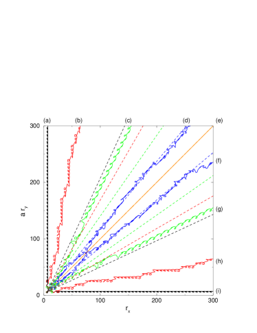
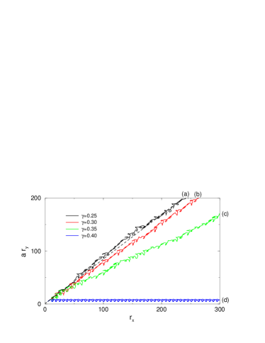
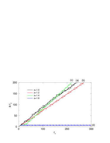
Figure 1: Top panel: Trajectories for a net force applied at different angles: $\theta=13\pi/36$ (a), $\pi/3$ (b), $11\pi/36$ (c), $5\pi/18$ (d), $\pi/4$ (e), $2\pi/9$ (f), $7\pi/36$ (g), $\pi/6$ (h), and $5\pi/36$ (i) for $a=1$ and $\gamma=0.25$. Medium panel: Trajectories for $a=1,\theta=2\pi/9$, and four values of the dimensionless coefficient of friction: $\gamma=0.25$ (a), $0.3$ (b), $0.35$ (c), and $0.4$ (d). Bottom panel: Trajectories for $\theta=2\pi/9,\gamma=0.25$, and four values of the eccentricity parameter: $a=1$ (a), $1.2$ (b), $1.4$ (c), and $1.6$ (d). Other parameters are: $F_{0x}=0.28,F_{1}=1,$ and $\Omega_{x}=0.68$. Dotted lines indicate the direction of the external force.

Figure 2: Deflection angle vs coefficient of friction for two values of the eccentricity parameter: $a=1$ $\left(\Diamond\right),1.5$ $\left(\blacktriangle\right)$. The inset shows the deflection angle vs eccentricity parameter for $\gamma=0.2$. Other parameters are: $\theta=\pi/5,F_{0x}=0.28,F_{1}=1,\Omega_{x}=0.68$. The solid lines are solely plotted to guide the eye.

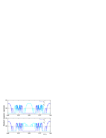
Figure 3: Maximal LEs $\Lambda_{x}^{+},\Lambda_{y}^{+}$ as a function of the angle $\theta$ for two values of the eccentricity parameter: $a=1$ (top panel), $1.5$ (bottom panel). Other parameters are: $F_{0x}=0.28,F_{1}=1,\gamma=0.25$ and $\Omega_{x}=0.68$.

Figure 4: Deflection angle vs external force direction for $F_{0x}=0.28,F_{1}=1,\Omega_{x}=0.68$, two values of the eccentricity parameter: $a=1$ (top panel), $1.5$ (bottom panel), and different values of the coefficient of friction: $\gamma=0.25\left(\Diamond\right),0.4\left(\blacktriangle\right)$ (top panel) and $\gamma=0.15\left(\Diamond\right),0.25\left(\blacktriangle\right)$ (bottom panel). Also plotted are the functions $-\tan\theta$ and $\cot\theta$ (dashed lines, see the text ).

Figure 1 (bottom panel) shows an illustrative example where typical trajectories are plotted for increasing values of $a$ from 1. Starting at a situation where CT occurs in both directions $\left(a=1\right)$, one finds that increasing the potential’s asymmetry $\left(a>1\right)$ changes the motion to PT in both directions (as for $a=1.2$). This behaviour changes again to CT in both directions for higher values of $a$ (as for $a=1.4$), and finally changes to PT in the $x$-direction while remain bounded inside a well in the $y$-direction (as for $a=1.6$). Also, the effectiveness of a fixed external force at sorting heavy particles is enhanced by breaking the potential symmetry (recall that $\gamma\sim m^{-1/2}$, see Fig. 2). Figure 3 shows illustrative instances of maximal LEs, $\Lambda_{x}^{+}$ and $\Lambda_{y}^{+}$, which quantify the chaotic dynamics in the $x$- and $y$-directions, respectively, versus $\theta$ for two values of the eccentricity parameter. Remarkably, these diagrams present relevant symmetries which are coherent with those of the chaotic threshold amplitudes [Eqs. (10)-(13), respectively]: $\Lambda_{x}^{+}\left(\pi/2\pm\theta\right)=\Lambda_{x}^{+}\left(\pi/2\mp\theta\right)$, $\Lambda_{y}^{+}\left(\pi/2\pm\theta\right)=\Lambda_{y}^{+}\left(\pi/2\mp\theta\right)$, $\Lambda_{x}^{+}\left(\pi/4\pm\theta\right)=\Lambda_{y}^{+}\left(\pi/4\mp\theta\right)$, $\Lambda_{x}^{+}\left(3\pi/4\pm\theta\right)=\Lambda_{y}^{+}\left(3\pi/4\mp\theta\right)$. It is worth mentioning that this coherence is far from trivial in the sense that, to the best of our knowledge, there is no theoretical connection between MA predictions and LEs for the present system, thus indicating the relevance and depth of the chaotic threshold symmetries in parameter space. One typically finds how different chaotic and non-chaotic regimes drastically change over certain $\theta$ ranges as the potential becomes asymmetric. For instance, PT in both directions at $\theta=\left\{\pi/4,3\pi/4\right\}$ for a symmetric potential $\left(a=1\right)$ changes to CT in solely one direction for an asymmetric potential $\left(a=1.5\right)$ (cf. Fig. 3). Finally, numerical simulations confirmed the accuracy of predictions (14) and (15) as is shown in Fig. 4. Starting with CT in both directions at $\theta=\pi/4$ for a symmetric potential (Fig. 4, top panel), one sees that the deflection of particles increases as $\theta$ deviates from $\pi/4$ according to the route described in Fig. 1, top panel. Maximum deflection occurs at symmetric angles with respect to $\pi/4,\theta_{\max}^{low},\theta_{\max}^{\sup}\left(\pi/4-\theta_{\max}^{low}\simeq\theta_{\max}^{\sup}-\pi/4\right)$, where there is PT in one direction while periodic oscillation in the other. For $\theta\geqslant\theta_{\max}^{\sup}$ $\left(\theta\leqslant\theta_{\max}^{low}\right)$, this transport regime remains, i.e., $\left\langle v_{x}\right\rangle=0$ $\left(\left\langle v_{y}\right\rangle=0\right)$ and hence $\tan\alpha\left(\theta\geqslant\theta_{\max}^{\sup}\right)=\cot\theta$ $\left(\tan\alpha\left(\theta\leqslant\theta_{\max}^{low}\right)=-\tan\theta\right)$ (cf. Eq. (7)). For an asymmetric potential (Fig. 4, bottom panel), the dependence of the deflection angle on the external force direction essentially presents a similar scenario to that of the symmetric case, but now $\tan\alpha$ is no longer an odd function with respect $\pi/4$, as predicted (cf. third remark).

Conclusions.$-$To sum, we have demonstrated theoretically and numerically through a simple and general system that reliable control of sorting on periodic surfaces is achieved for chaotic particles by identifying the relevant symmetries of the chaotic threshold in parameter space. We uncovered and characterized different sorting scenarios associated with symmetric and asymmetric spatial potentials, which could motivate experiments in different contexts such as optical and antidot lattices. Among the most interesting extensions of this work are the case with the ac and dc forces having different directions, where preliminary results indicate the presence of intriguing “absolute negative mobility” phenomena 18 , as well as the study of the effect of noise on the present transport scenarios: Even very small amounts of noise may cause both a transition from a bounded state to a running state and a significative modification of the chaotic threshold in parameter space 19 . Our current work is aimed at exploring these cases.

We thank Katja Lindenberg for useful discussions. This work was partially supported by the Ministerio de Ciencia e Innovación (MCINN, Spain) under projects FIS2008-01383 (R. Ch.) and FIS2009-13360-C03-03 (A.M.L.).

References

(1) H. Risken, The Fokker-Planck Equation (Springer,
Berlin, 1984), Chap. 11.
(2) P. T. Korda, M. B. Taylor, and D. G. Grier, Phys. Rev. Lett.
89, 128301 (2002).
(3) C. Reichhardt and F. Nori, Phys. Rev. Lett. 82, 414
(1999).
(4) J. W. Reijnders and R. A. Duine, Phys. Rev. Lett. 93,
060401 (2004).
(5) A. W. Ghosh and S. V. Khare, Phys. Rev. Lett. 84, 5243
(2000).
(6) J. D. Bao and Y. Z. Zhuo, Phys. Lett. A 239, 228 (1998).
(7) I. Derényi and R. D. Astumian, Phys. Rev. E 58,
7781 (1998).
(8) R. Eichhorn, P. Reimann, and P. Hänggi, Phys. Rev. Lett.
88, 190601 (2002).
(9) R. Guantes and S. Miret-Artés, Phys. Rev. E 67,
046212 (2003).
(10) A. M. Lacasta, J. M. Sancho, A. H. Romero, and K. Lindenberg,
Phys. Rev. Lett. 94, 160601 (2005).
(11) J. P. Gleeson, J. M. Sancho, A. M. Lacasta, and K. Lindenberg,
Phys. Rev. E 73, 041102 (2006).
(12) S. Denisov, Y. Zolotaryuk, S. Flach, and O. Yevtushenko, Phys.
Rev. Lett. 100, 224102 (2008).
(13) M. Khoury, A.M. Lacasta, J.M Sancho, A.H. Romero, K. Lindenberg,
Phys. Rev. B 78, 155433 (2008), and references therein.
(14) V. K. Melnikov, Trans. Moscow Math. Soc. 12, 1 (1963).
(15) See, e.g., A. J. Lichtenberg and M. A. Lieberman, Regular and Chaotic Dynamics (Springer, New York, 1992), Chaps. 5 and 7.
(16) J. Guckenheimer and P. J. Holmes, Nonlinear
Oscillations, Dynamical Systems, and Bifurcations of Vector Fields
(Springer, Berlin, 1983).
(17) G. Grynberg and C. Robilliard, Phys. Rep. 355, 335
(2001).
(18) D. Speer, R. Eichhorn, and P. Reimann, Phys. Rev. Lett. 102, 124101 (2009).
(19) P. J. Martínez and R. Chacón, Phys. Rev. Lett. 93, 237006 (2004).