Universal conductance enhancement and reduction of the two-orbital Kondo effect

Abstract

We investigate theoretically the linear and nonlinear conductance through a nanostructure with two-fold degenerate single levels, corresponding to the transport through nanostructures such as a carbon nanotube, or double dot systems with capacitive interaction. It is shown that the presence of the interaction asymmetry between orbits/dots affects significantly the profile of the linear conductance at finite temperature, and, of the nonlinear conductance, particularly around half-filling, where the two-particle Kondo effect occurs. Within the range of experimentally feasible parameters, the $SU(4)$ universal behavior is suggested, and comparison with relevant experiments is made.

1 Introduction

Electrical transport through nanostructure devices or a quantum dot is fundamentally influenced by the presence of the Coulomb interaction on the dot, where along with the Coulomb blockade phenomena, the Kondo effect, a paradigm of the strongly correlated phenomena, has been observed [1]. The great advantage of these nanostructure systems is the ability to control various relevant parameters to regulate many-body effect. Toward future applications of quantum electron devices, interest in a role of many-body effect of the transport phenomena has been rekindled and studies have been made actively.

In the absence of magnetic field, the levels of a quantum dot are spin degenerate; the Kondo effect gives rise to the conductance enhancement at low-temperatures in an odd electron number on the dot, as a result of the interaction between a local magnetic moment of the dot and conduction electrons. The spin degree can be replaced by another degenerate degrees of freedom. Indeed, two quantum dots with capacitive interaction can be labeled by an index $i=1,2$, which can be taken as another realization of the Anderson impurity model [2]; the orbital Kondo effect appears [3, 4, 5, 6, 7, 8, 9, 10]. Other notable examples are vertical quantum dots [11], or carbon nanotube dots [12, 13, 14, 15]. All of these systems accommodate one, two, three, four electrons in the topmost shell, and the Coulomb blockade peaks show a clear sign of the fourfold pattern. When the spin and orbital degeneracies are simultaneously present, the further entanglement between spin and orbital degrees of freedom occurs, giving rise to the $SU(4)$ Kondo effect with an Kondo temperature one order of magnitude higher than the standard case [9, 10, 16, 17, 18, 3, 4, 14, 15].

Though most of studies of the systems with doubly degenerate orbitals have been focusing on odd-number valleys ($N_{d}\approx 1$ or $3$), it has been recognized recently that a similar Kondo-like enhancement (two-particle $SU(4)$ Kondo effect) can occur on even-number valley ($N_{d}\approx 2$) as well [19, 20] (See also ref. Eto00 for the singlet-triplet Kondo effect.) However, such enhancement at even-number valleys does not seem ubiquitous, observed in some experiments but not in others. The conductance of carbon nanotube dots fits well with $G\propto\sin^{2}(\pi N_{d}/4)$ at very low temperature [15], which shows the Kondo enhancement both at odd and even valleys; but in two coupled dots, the honeycomb-like structure as a function of the two gate voltages shows the enhancement at $N_{d}=1$ but not at $N_{d}=2$.

In this paper, we will examine the quantum transport through a dot with doubly degenerate orbitals with different interaction strengths within the orbits and between orbits. We will show that such interaction asymmetry, if small, is important to understand the profile of the linear conductance at finite temperature, and, of the nonlinear conductance. Resorting to the universality of the topmost shell, the $SU(4)$ Anderson model, we analyze how the conductance gets enhanced or suppressed at finite temperature or by finite source-drain voltage. Though the conductance profiles observed in several experiments may seem nonuniversal at first glance, we will find that we can explain them systematically by the $SU(4)$ Anderson model universality, once taking proper account of the presence of the interaction asymmetry between orbits/dots.

We are concerned particularly with the universal dependence of the temperature and/or the bias voltage of the conductance. Naively, one may expect the singlet-triplet Kondo effect at half-filling when the interaction asymmetry is present. On the other hand, even with the interaction asymmetry, the renormalization group (RG) flow is known to drive the system toward the $SU(4)$-symmetric strong coupling point, either at quarter-filling or at half-filling [19, 20]. Because of it, it is unclear what is the relevant symmetry of the system once interaction asymmetry is present; the unitarity limit of the conductance enhancement at quarter-filling cannot distinguish between them. In the standard spin-degenerate $SU(2)$ Kondo systems, experiments have confirmed universal scaling regarding temperature [22] as well as the bias voltage at odd valleys [23, 24]. Since the absence of the exact $SU(4)$ symmetry exhibits the behavior at finite temperature and/or at finite bias voltage, we will try to identify the relevant universality, $SU(4)$ or $SU(2)\times SU(2)$, by examining the universal scaling of the linear/nonlinear conductance. We will show numerically no crossover observed in the conductance for a experimentally relevant parameters $U^{\prime}/U=0.4\sim 1.0$ and $U=10\sim 20\Gamma$; the Kondo-like enhancement is controlled by the universal behaviors of the $SU(4)$ Anderson model only with the characteristic temperature renormalized.

Outline of the paper

The paper is organized as follows. In Sec. 2, we introduce the model of quantum transport through a nanostructure with two-fold degenerate orbits, and main apparatus of our approach, finite interaction slave-boson mean field theory; a brief theory of the linear/nonlinear conductance is summarized. In Sec. 3, we present our theoretical results both for the linear and nonlinear conductance. We see the importance of the interaction asymmetry on the conductance profile. A direct comparison with numerical RG data is also made. After introducing the characteristic temperature $T^{*}$ in Sec. 4, we discuss our theoretical results in light of $T^{*}$, and universal scalings of linear and nonlinear conductance is examined in Sec. 5. After discussing an issue of $T^{*}$ renormalization versus a crossover in Sec. 6, we compare and discuss our results with typical experiments where the interaction asymmetry is expected to play an important role in Sec. 7. Finally we conclude in Sec. 8. Part of the results on the linear conductance has been reported earlier [25].

2 Model and Formulation

2.1 Quantum dots with doubly degenerate orbitals

Relatively large energy scale of the Coulomb interaction allows us to focus on the topmost electron shell. Our basic assumption is that within the universality of the topmost shell, the Anderson impurity model can describe appropriately quantum transport phenomena for any value of $N_{d}$. We model the topmost shell of the dot as degenerate in orbits $i=1,2$. Such degeneracy may come from the coupled-dot or a unique electronic structure of carbon nanotubes.

On the dot, an electron interacts with an electron in the same orbit $i=1,2$ by $U$ or in the different orbit by $U^{\prime}$. The total Hamiltonian is given by

$$H=H_{D}+H_{L}+H_{T},$$ (1)

where the dot $H_{D}$, the noninteracting leads $H_{L}$, and the coupling between leads ($\alpha=L,R$) and the dot $H_{T}$ are defined by

$$H_{D}=\sum_{i\sigma}\varepsilon_{d}\,\hat{n}_{i\sigma}+\sum_{i}U\hat{n}_{i\uparrow}\hat{n}_{i\downarrow}+U^{\prime}\hat{n}_{1}\hat{n}_{2},$$ (2)

$$H_{L}=\sum_{\alpha}\sum_{ki\sigma}\left(\varepsilon_{k}-\mu_{\alpha}\right)c^{\dagger}_{\alpha ki\sigma}c_{\alpha ki\sigma},$$ (3)

$$H_{T}=\sum_{\alpha}\sum_{ki\sigma}\left(t_{k}c^{\dagger}_{\alpha ki\sigma}d_{i\sigma}+\text{h.c.}\right).$$ (4)

Here the number operator of the dot is defined by $\hat{n}_{i}=\sum_{\sigma}\hat{n}_{i\sigma}=\sum_{\sigma}d^{\dagger}_{i\sigma}d_{i\sigma}$ and the gate voltage $\varepsilon_{d}$ control the average electron number on the dot $N_{d}=\langle\sum_{i}\hat{n}_{i}\rangle$ continuously from $0$ to $4$. In the calculation below, we assume constant density of states $\rho_{\alpha}$ of the lead $\alpha$ within the energy band $(-D,D)$, and use $\Gamma=\sum_{\alpha}\Gamma_{\alpha}=\sum_{\alpha}\pi\rho_{\alpha}|t_{k}|^{2}$ as a coupling parameter between the leads and the dot. To investigate the nonlinear conductance in the presence of finite source-drain voltage $V$, we choose the chemical potentials $\mu_{\alpha}$ as $\mu_{L}=-\mu_{R}=eV/2$.

In the case of $U^{\prime}=U$, the total Hamiltonian $H$ exhibits the full $SU(4)$ symmetry. The states $(n_{1},n_{2})=(1,0)$ and $(0,1)$ are four-fold degenerate at quarter-filling ($N_{d}=1$); $(n_{1},n_{2})=(2,0)$, $(1,1)$ and $(0,2)$, six-fold degenerate at half-filling ($N_{d}=2$).

When one breaks the $SU(4)$ symmetry by decreasing $U^{\prime}$, the four-fold degeneracy at quarter-filling is unbroken, but the six-fold degeneracy at half-filling is broken. The effect of the interaction asymmetry appears as shifts of the Coulomb blockade peaks, those at $\varepsilon_{d}=0$, $-U^{\prime}$, $-U-U^{\prime}$, and $-U-2U^{\prime}$. However, the effect of the interaction asymmetry does not stop here; it gives a substantial effect in the Kondo effect particularly at half-filling. This simple argument also indicates that the $SU(4)$ symmetry at half-filling is more vulnerable than that at quarter-filling. We will show below that this is indeed the case.

2.2 Finite-interaction slave-boson mean-field theory

We analyze the model by an extension of the Kotliar-Ruckenstein formulation of slave-boson mean field theory (KR-SBMT) [26], where a bosonic field is attached to each type of local excitations. [27] The approach has several advantages that other slave-boson cousins miss. By retaining finite interaction, it can treat the mixed-valence regime; it applies to nonlinear transport through a quantum dot [28]; it reproduces Fermi liquid behavior at $T=0$ with satisfying the Friedel sum rule; it can evaluate the linear/nonlinear conductance for the entire range of the gate voltage systematically. The KR formulation of SBMT is believed to be an analytical yet reliable non-perturbative approximation up to the Kondo temperature, agreeing successfully with numerical RG methods and experiments [28, 29] (see also Sec. 3).

When the KR-SBMT is extended to the dot with doubly degenerate orbitals, 16 bose fields are needed associated to each state of the dot: $e$ for the empty, $p_{i\sigma}$ for one electron with orbit $i$ and spin $\sigma$, $x_{i}$ for two electrons on the same orbit $i$, $y_{sm}$ for two electrons at different orbits with total spin $(s,m)$, $h_{i\sigma}$ for three electrons with a hole on $i\sigma$, and $b$ for fully occupied state. Below we briefly summarize our approximation scheme (see also ref. Dong02).

As a standard treatment of the Kotliar-Ruckenstein formulation, we can rewrite the Hamiltonian eq. (1) in terms of these newly defined fields by adding the Lagrange multiplier terms $H_{\Lambda}=\lambda^{(1)}(\mathcal{I}-1)+\sum_{i\sigma}\lambda^{(2)}_{i\sigma}\left(d^{\dagger}_{i\sigma}d_{i\sigma}-Q_{i\sigma}\right)$ to respect two constraints: the completeness condition,

$$\mathcal{I}\equiv e^{\dagger}e+\sum_{i\sigma}p^{\dagger}_{i\sigma}p_{i\sigma}+\sum_{i}x^{\dagger}_{i}x_{i}$$

$$\quad+\sum_{sm}y^{\dagger}_{sm}y_{sm}+\sum_{i\sigma}h^{\dagger}_{i\bar{\sigma}}h_{i\bar{\sigma}}+b^{\dagger}b=1,$$ (5)

and the number correspondence between fermions and newly defined bosons,

$$\mathcal{Q}_{i\sigma}\equiv p^{\dagger}_{i\sigma}p_{i\sigma}+x^{\dagger}_{i}x_{i}+y^{\dagger}_{1,2\sigma}y_{1,2\sigma}+\frac{1}{2}(y^{\dagger}_{00}y_{00}+y^{\dagger}_{10}y_{10})$$

$$\quad+h^{\dagger}_{i\bar{\sigma}}h_{i\bar{\sigma}}+\sum_{\sigma^{\prime}}h^{\dagger}_{\bar{i}\sigma^{\prime}}h_{\bar{i}\sigma^{\prime}}+b^{\dagger}b=d^{\dagger}_{i\sigma}d_{i\sigma}.$$ (6)

Here and hereafter, we adopt the notation $\bar{1}=2$, $\bar{2}=1$, $\bar{\uparrow}=\downarrow$, $\bar{\downarrow}=\uparrow$. As a result, we can rewrite eq. (1) exactly as

$$H=H_{L}+\sum_{i\sigma}\varepsilon_{d}\,d^{\dagger}_{i\sigma}d_{i\sigma}+U\sum_{i}x^{\dagger}_{i}x_{i}+U^{\prime}\sum_{sm}y^{\dagger}_{sm}y_{sm}$$

$$\quad+(U+2U^{\prime})\sum_{i\sigma}h^{\dagger}_{i\sigma}h_{i\sigma}+(2U+4U^{\prime})b^{\dagger}b$$

$$\quad+\sum_{ki\sigma}\left(t_{k}c^{\dagger}_{ki\sigma}d_{i\sigma}z_{i\sigma}+\text{h.c.}\right)+H_{\Lambda},$$ (7)

where $z_{i\sigma}=(1-Q_{i\sigma})^{-\frac{1}{2}}[e^{\dagger}p_{i\sigma}+p^{\dagger}_{i\bar{\sigma}}x_{i}+p^{\dagger}_{\bar{i}\sigma}y_{1,2\sigma}+p^{\dagger}_{\bar{i}\bar{\sigma}}(y_{00}+y_{10})/{2}+x^{\dagger}_{\bar{i}}h_{i\bar{\sigma}}+(y^{\dagger}_{00}+y^{\dagger}_{10})h_{\bar{i}\bar{\sigma}}/2+y^{\dagger}_{1,2\bar{\sigma}}h_{\bar{i}\sigma}+h^{\dagger}_{i\sigma}b]Q_{i\sigma}^{-\frac{1}{2}}$ denotes a renormalization of one-particle annihilation.

By applying the mean field approximation, we replace all the boson fields by their expectation values. We determine those expectation values self-consistently by solving equations of motion and constraints at each gate voltage $\varepsilon_{d}$, the bias condition $V$ and the temperature $T$. By adopting a symmetric solution regarding the orbit $i$ and the spin $\sigma$, we should solve the following self-consistent equations (omitting spin/orbit indices),

$$4\frac{\partial\ln z}{\partial e}M+\lambda^{(1)}\,e=0,$$ (8)

$$\frac{\partial\ln z}{\partial p}M+(\lambda^{(1)}-\lambda^{(2)})p=0,$$ (9)

$$2\frac{\partial\ln z}{\partial x}M+(U+\lambda^{(1)}-2\lambda^{(2)})x=0,$$ (10)

$$\frac{\partial\ln z}{\partial y}M+(U^{\prime}+\lambda^{(1)}-2\lambda^{(2)})y=0,$$ (11)

$$\frac{\partial\ln z}{\partial h}M+(U+2U^{\prime}+\lambda^{(1)}-3\lambda^{(2)})h=0,$$ (12)

$$4\frac{\partial\ln z}{\partial b}M+(2U+4U^{\prime}+\lambda^{(1)}-4\lambda^{(2)})b=0,$$ (13)

as well as two constraints

$$e^{2}+4p^{2}+2x^{2}+4y^{2}+4h^{2}+b^{2}=1,$$ (14)

$$N_{d}/4=p^{2}+x^{2}+2y^{2}+3h^{2}+b^{2}.$$ (15)

Here we have introduced (non-equilibrium) Green functions $G^{<}_{d}(t,t^{\prime})\equiv i\langle d^{\dagger}_{i\sigma}(t^{\prime})d_{i\sigma}(t)\rangle$, its Fourier transformation $G^{<}_{d}(\omega)$, and $M=\int\frac{d\omega}{2\pi i}(\omega-\tilde{\varepsilon}_{d})G^{<}_{d}(\omega)$.

2.3 Current formula and nonlinear conductance

On determining these auxiliary parameters self-consistently at each temperature and each gate voltage, the system reduces to the renormalized resonant level model

$$H_{\text{eff}}=H_{L}+\sum_{i}\tilde{\varepsilon}_{d}\,\hat{n}_{i}+\sum_{\alpha ki\sigma}\left(\tilde{t}_{k}\,c^{\dagger}_{\alpha ki\sigma}d_{i\sigma}+\text{h.c.}\right),$$ (16)

with the effective dot level $\tilde{\varepsilon}_{d}=\varepsilon_{d}+\lambda^{(2)}$ and the effective hopping $\tilde{t}_{k}=zt_{k}$, which corresponds to the effective peak width $\tilde{\Gamma}=\tilde{\Gamma}_{L}+\tilde{\Gamma}_{R}=\sum_{\alpha}\pi\rho_{\alpha}|\tilde{t}_{k}|^{2}$. The effective Hamiltonian conforms to Fermi liquid description at low temperature, the strong-coupling fixed point. Note that interaction effect is considered only through $\tilde{\varepsilon}_{d}$, $\tilde{t}_{k}$ and we ignore a remaining (renormalized) interaction term between quasiparticles.

The form of $H_{\text{eff}}$ enables us to find the linear/nonlinear conductance by the Meir-Wingreen formula [31]:

$$I=\frac{16e\tilde{\Gamma}_{L}\tilde{\Gamma}_{R}}{h}\int d\omega\,\frac{\left[f_{L}(\omega)-f_{R}(\omega)\right]}{(\omega-\tilde{\varepsilon}_{d})^{2}+\tilde{\Gamma}^{2}}$$ (17)

$$\quad=\frac{4G_{0}\tilde{\Gamma}}{e}\mathop{\mathrm{Im}}\nolimits\left[\psi\left(\tfrac{1}{2}+i\zeta_{R}\right)-\psi\left(\tfrac{1}{2}+i\zeta_{L}\right)\right],$$ (18)

where $f_{\alpha}(\omega)=1/[e^{(\omega-\mu_{\alpha})/T}+1]$ is the Fermi distribution function of the lead, $G_{0}=(4\tilde{\Gamma}_{L}\tilde{\Gamma}_{R}/\tilde{\Gamma}^{2})(e^{2}/h)$, $\zeta_{\alpha}=(\tilde{\varepsilon}_{d}-\mu_{\alpha}-i\tilde{\Gamma})/(2\pi T)$, and $\psi$ is the digamma function. By this, we can readily evaluate the nonlinear conductance at finite bias voltage $V$ by

$$G(T,V)=\frac{dI}{dV}.$$ (19)

We should bear in mind, however, that the renormalized parameters $\tilde{\varepsilon}_{d}$ and $\tilde{\Gamma}$ still depend on $V$ as well as $T$ and interaction strengths.

At $T=0$, the electron number on the dot is equal to $N_{d}=2-\frac{4}{\pi}\arctan\big{(}\tilde{\varepsilon}_{d}/\tilde{\Gamma}\big{)}$. This immediately shows that the linear conductance at zero temperature $G(0,0)$ satisfies

$$G(0,0)=4G_{0}\sin^{2}(\pi N_{d}/4).$$ (20)

This is the Friedel sum rule of the $SU(4)$ Anderson model. The formula immediately indicates that the zero-bias conductance in the unitarity limit approaches $G(0,0)\to 2G_{0}$ at $N_{d}=1,3$, but $G(0,0)\to 4G_{0}$ at $N_{d}=2$. The observation of the above dependence of $G(0,0)$ on continuous $N_{d}$ is a hallmark of the $SU(4)$ Anderson model; a recent experiment [15] and calculations by numerical RG [32] confirmed it beautifully.

3 Linear and nonlinear conductance

In this section, we present our main numerical results of linear/nonlinear conductance as a function of the temperature and/or bias voltage. The Friedel sum rule indicates the zero-bias conductance at $T=0$ does not depend on interaction asymmetry, taking a universal form, eq. (20). Accordingly, the absence of the exact $SU(4)$ symmetry appears at finite temperature and/or bias-voltage; we will find that the effect is large enough to modify the conductance profile substantially, providing a characteristic ‘dip structure’ around half-filling. For all the calculations, we fix a parameter $U/\Gamma=20$ as a typical value of strong correlation in experiments, and we take $U$ as a unit energy scale, if needed.

3.1 $G(T,0)$ of symmetric interaction $U^{\prime}=U$; comparison with NRG results

As a first step, we compare the zero-bias conductance $G(T,0)$ obtained by our KR-SBMT approach with the NRG calculations available for the $SU(4)$ Anderson model with symmetric interaction $U^{\prime}=U$ [32]. We find that our results reproduce NRG data quite well.

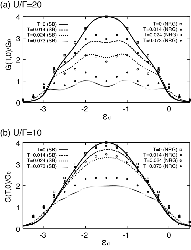
Figure 1: Comparison between the KR-SBMT and numerical RG results [32]. Temperature evolution of linear conductance $G(T,0)$ is plotted as a function of the gate voltage for the fully symmetric $SU(4)$ Anderson model. (a) SBMT results (lines) of $U/\Gamma=20$ are compared with NRG data (symbols) of $U/\Gamma=10$; (b) SBMT results (lines) of $U/\Gamma=10$, with NRG data (symbols) of $U/\Gamma=5$ (see the text for details).

Figure 1 (a) demonstrates a distinctive feature of the conductance profile in large $U/\Gamma$ region, the Kondo enhancement both at $N_{d}\approx 2$ and at $N_{d}\approx 1$; with increasing temperature, the four-fold Coulomb blockade peaks appear. Regarding the mixed-valence regime with a smaller value of $U/\Gamma$, four-fold peaks merge to form one big peak showing the Kondo enhancement (see Fig. 1 (b)). As was claimed already [32], these temperature evolutions by $SU(4)$ symmetric Anderson model agree very well with what is observed either at $V_{g}\sim 3.9\textrm{V}$ or at $V_{g}\sim 5.3\textrm{V}$ in an experiment [15].

Our KR-SBMT results agree even quantitatively well with NRG results, but with one catch: In comparing with NRG data, we need to resort to a heuristic prescription choosing the twice as large value of $U/\Gamma$ for the SBMT results. [33] Indeed, the same problem has been prevailing in the single impurity Anderson model; we can attain quantitative agreement between effective theories (the KR-SBMT [29] or the functional RG [34]) and the NRG method only if we choose the twice as large value of $U/\Gamma$ for the former. Figure 1 shows comparison by using this heuristic prescription, and they agree very well in low temperature, roughly up to the Kondo temperature scale.

3.2 Effect of interaction asymmetry on $G(T,0)$

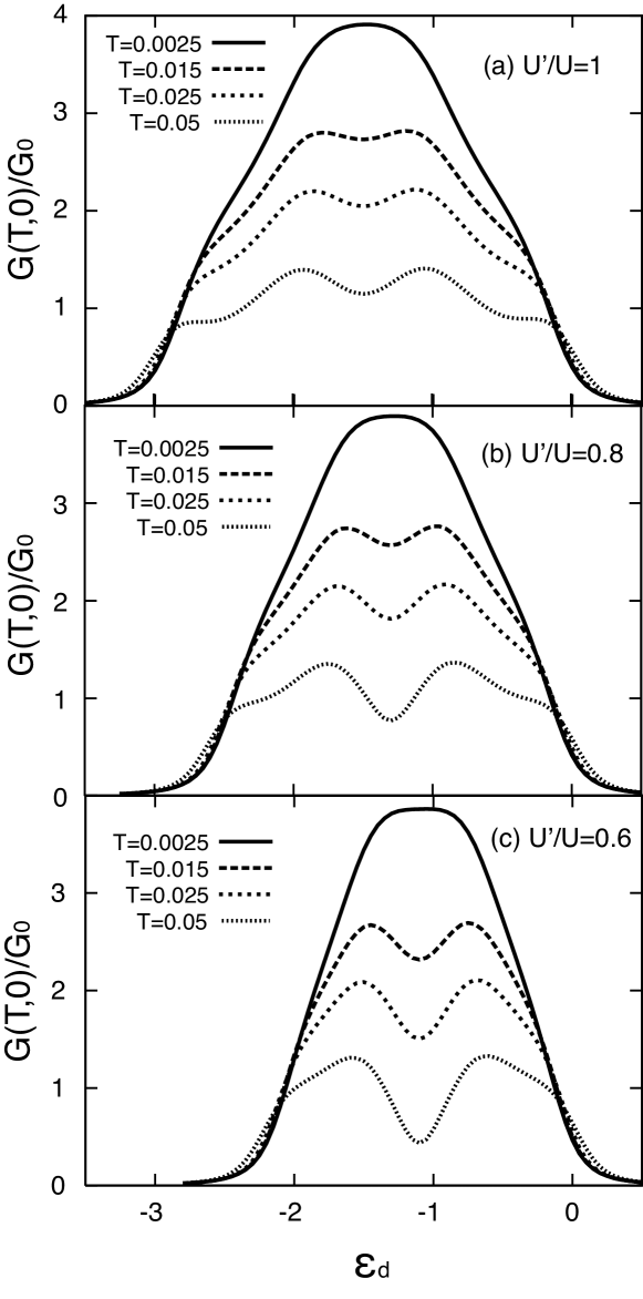
Figure 2: The temperature evolutions of the conductance $G(T,0)$ as a function of the gate voltage with varying asymmetry $U^{\prime}/U=1$, $0.8$, and $0.6$.

Figure 2 demonstrates typical temperature evolutions of the conductance profile as a function of the gate voltage with varying asymmetry parameters (a) $U^{\prime}/U=1$, (b) $0.8$, and (c) $0.6$. Overall widths of conductance profiles are determined by $U+2U^{\prime}$. We notice, even with a small asymmetry $U^{\prime}/U=0.8$, a characteristic dip structure of $G(T,0)$ developing clearly at half-filling ($N_{d}=2$) at finite temperature, in contrast with a small deformation around quarter and three-quarter-fillings ($N_{d}=1,3$). Recall for any finite $0<U^{\prime}<U$, the system is always renormalized to the $SU(4)$ symmetric model [19, 20] and the Kondo enhancement always appear at the gate voltage corresponding to $N_{d}=1,2,3$; $G(0,0)$ is determined by the Friedel sum rule eq. (20) irrespective of the interaction asymmetry. We stress the interaction asymmetry manifests itself only at finite temperature and invisible at $T=0$. It appears as a substantial ‘dip structure’ of $G(T,0)$ around half-filling. As we have claimed recently [25], such feature caused by interaction asymmetry reproduces quite well experimental observation in carbon nanotube dots [14, 15] (see Sec. 7 for more details).

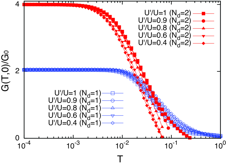
Figure 3: (color online) Temperature dependence of the conductance $G(T,0)$ as a function of the interaction asymmetry $U^{\prime}/U=1$, $0.9$, $0.8$, $0.6$, and $0.4$ at $N_{d}=1$ (quarter-filling) and at $N_{d}=2$ (half-filling).

To clarify how the asymmetric interaction affect the conductance profile particularly at half-filling, we make a direct comparison between the behaviors at $N_{d}=1$ and $N_{d}=2$ in Fig. 3 by changing $U^{\prime}/U=1$, $0.9$, $0.8$, $0.6$, and $0.4$. By decreasing $U^{\prime}$ away from the symmetric point $U^{\prime}=U$, the characteristic energy controlling thermal suppression seems reduced at $N_{d}=2$, but enhanced at $N_{d}=1$. We will elucidate this tendency by estimating $T^{*}$ numerically in Sec. 4.

3.3 Effect of interaction asymmetry on $G(0,V)$

We now turn our attention to the non-equilibrium transport, i.e., nonlinear conductance. To understand the interplay between finite bias voltage effect and the interaction asymmetry, we here examine the zero-temperature differential conductance $G(0,V)$.

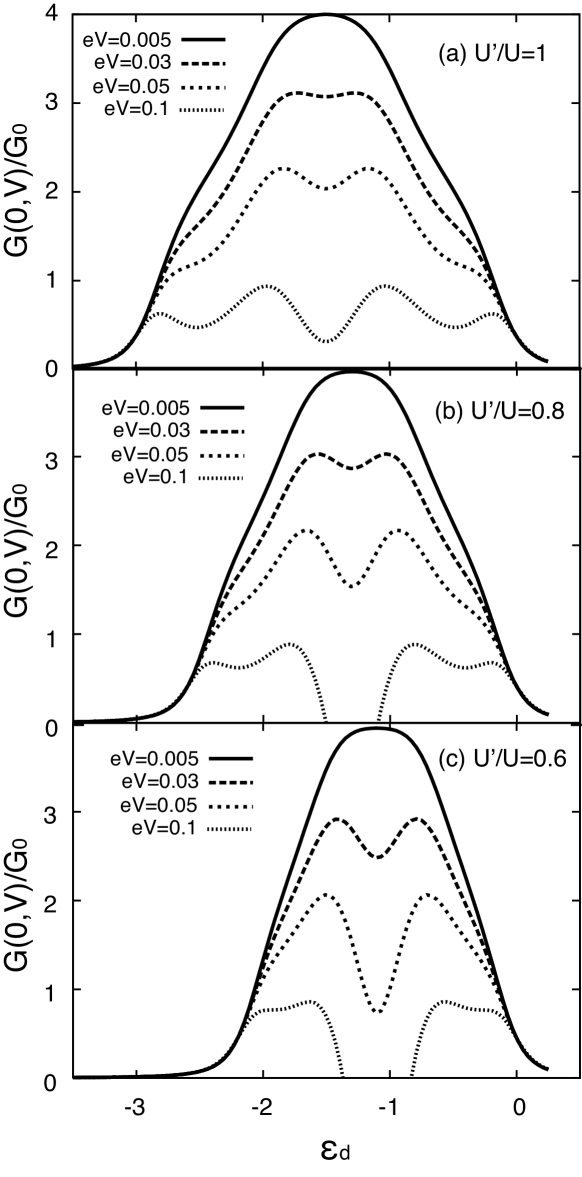
Figure 4: Bias voltage evolution of the zero-temperature differential conductance $G(0,V)$ as a function of the gate voltage with varying the interaction asymmetry (a) $U^{\prime}/U=1$, (b) $U^{\prime}/U=0.8$, and (c) $U^{\prime}/U=0.6$.

Figure 4 shows typical bias voltage evolutions of $G(0,V)$ as a function of the gate voltage with asymmetry parameters (a) $U^{\prime}/U=1$, (b) $0.8$, and (c) $0.6$. We immediately notice that the profile of $G(0,V)$ looks quite similar to that of $G(T,0)$. By applying larger bias voltage ($eV/U=0.03$, $0.05$, $0.1$), the Kondo enhancement both at $N_{d}=1,3$ and $N_{d}=2$ is suppressed, but the latter suppression is more distinctive. Like the thermal evolutions, the interaction asymmetry manifests itself only at a fixed finite bias voltage, as a ‘dip structure’ of $G(0,V)$ around half-filling.

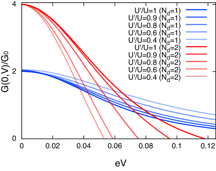
Figure 5: (color online) The differential conductance $G(0,V)$ as a function of the bias voltage with varying the interaction asymmetry $U^{\prime}/U=1,0.9,0.8,0.6,0.4$ at $N_{d}=2$ (approaching $G(0,V\to 0)\to 4G_{0}$), and at $N_{d}=1$ (approaching $G(0,V\to 0)\to 2G_{0}$).

Figure 5 shows the zero bias peak $G(0,V)$ either at $N_{d}=1$ or at $N_{d}=2$ with varying the asymmetry parameter $U^{\prime}/U=1.0$, $0.9$, $0.8$, $0.6$, and $0.4$. Since we assume the symmetric coupling $\Gamma_{L}=\Gamma_{R}$ to the leads, the $G(0,V)$ becomes symmetric regarding $V$. From its behavior, we can read off how the characteristic energy scale depends on the asymmetric parameter $U^{\prime}/U$. The dependence is the same with what is observed in the temperature evolutions of $G(T,0)$; decreasing $U^{\prime}$ leads to the reduction of the characteristic energy at $N_{d}=2$, but the enhancement at $N_{d}=1$.

Our numerical calculations show that the conductance at $N_{d}=2$

4 Characteristic temperature $T^{*}$

The Kondo temperature is an energy scale characterizing the Kondo effect, i.e., the Anderson model eq. (1) at the center of an odd Coulomb blockade valley. It is a crossover temperature, not the transition temperature, so we can fix it only modulo numerical factor with ambiguity. Instead, we seek to define a characteristic energy scale at each gate voltage covering the entire range of the topmost shell.

Recalling the present effective theory expresses the dot Green function as

$$G^{R}_{d}(\omega=0)=\frac{1}{-\tilde{\varepsilon}_{d}+i\tilde{\Gamma}}=-\frac{\exp(i\pi N_{d}/4)}{\sqrt{\tilde{\varepsilon}_{d}^{2}+\tilde{\Gamma}^{2}}},$$ (21)

we naturally define a characteristic temperature $T^{*}$ of the model

$$T^{*}=\sqrt{\tilde{\varepsilon}_{d}^{2}+\tilde{\Gamma}^{2}}\,\Big{|}_{T=0,V=0}$$ (22)

at each gate voltage or $N_{d}$. We stress it is imperative to include the shift $\tilde{\varepsilon}_{d}$ in defining a consistent energy scale at each $N_{d}$.

When $\tilde{\varepsilon}_{d}$ vanishes, we see $T^{*}=\tilde{\Gamma}$, the Kondo peak width. This is a situation of the $SU(2)$ Kondo effect. However, as derived from the Friedel sum rule of $SU(4)$ model, eq. (20), the $SU(4)$ Kondo peak needs to shift at the $N_{d}=1,3$ [17, 18] by $|\tilde{\varepsilon}_{d}|=\tilde{\Gamma}=T^{*}/\sqrt{2}$. In contrast, the $SU(4)$ Kondo peak at $N_{d}=2$ does not shift because of the electron-hole symmetry.

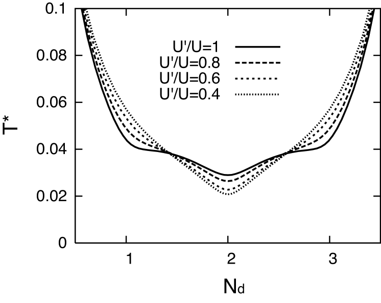
Figure 6: Dependence of the characteristic temperature $T^{*}$ on the average electron number of the dot with varying interaction asymmetry $U^{\prime}/U$.

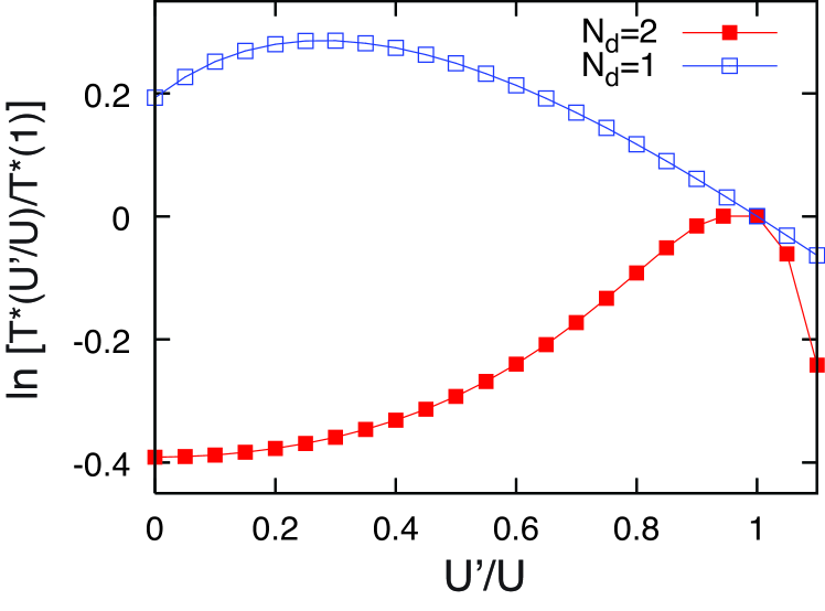
Figure 7: (color online) Dependence of the characteristic temperature $T^{*}$ on the interaction asymmetry $U^{\prime}/U$ for $N_{d}=2$ (filled square) and for $N_{d}=1$ (empty square).

The dependence of the characteristic energy $T^{*}$ obtained from our KR-SBMT calculations is shown in Fig. 6 for the entire range of the topmost shell ($N_{d}=0\sim 4$). Though the state degeneracy at $U^{\prime}=U$ is six-fold at $N_{d}=2$ and four-fold at $N_{d}=1$ respectively, $T^{*}$ of the former is lower than that of the latter.

The presence of the interaction asymmetry further amplifies this difference of $T^{*}$ as in Fig. 7; it reduces $T^{*}$ at $N_{d}=2$ but enhances it at $N_{d}=1$; $T^{*}$ is almost unchanged at the filling corresponding to Coulomb blockade peaks ($N_{d}\approx 1.3$ and $2.7$ in Fig. 6). Because of this, the Kondo enhancement around $N_{d}\approx 2$ is destroyed more rapidly than at $N_{d}\approx 1$ either by finite temperature or by finite bias voltage. The above dependence of $T^{*}$ gives a consistent explanation on the conductance profiles Figs. 2–5 in the previous section.

How much asymmetry deforms the conductance profile of the $SU(4)$ symmetry? The characteristic temperature $T^{*}$ at half-filling (of the symmetric model) controls it. When $|U-U^{\prime}|$ exceeds $T^{*}(N_{d}=2,U^{\prime}=U)$, it reduces $T^{*}$ rapidly, producing the conductance profile with a distinctive dip at half-filling. One can observe the effect only at finite temperature or by finite bias voltage. The above behavior of $T^{*}$ at $N_{d}=1$, $2$ agrees qualitatively with other numerical estimates of the Kondo temperature [19, 20, 35, 36]. However, we need to distinguish between the reduction of the characteristic energy and the crossover between the universality classes: the former does not necessarily mean the latter. We will focus on the issue in next section.

5 Universal scaling of linear and nonlinear conductance

Having understood qualitative behavior of the conductance profiles by temperature or bias voltage, we now focus on examining an important issue: what is the universality controlling quantum transport in the presence of the interaction asymmetry? The nature at half-filling have been argued actively so far, proposing the $SU(2)\times SU(2)$ Kondo effect [19, 20, 35], or the $SU(4)$ Kondo effect [36]. We should bear in mind that the absence of the exact $SU(4)$ symmetry of the model does not necessarily legitimate the former universality, because the model flows toward the $SU(4)$ symmetric strong coupling point for $0<U^{\prime}<U$; neither the reduction of $T^{*}$ in Fig. 7.

When the nonlinear conductance $G(T,V)$ is dominated by a unique universality, we expect to express $G(T,V)$ by some universal function $F_{n}(t=T/T^{*},v=eV/T^{*})$ at each filling $n=N_{d}$:

$$G(T,V)/G_{0}=F_{n}(t,v).$$ (23)

The Friedel sum rule eq. (20) constrains $F_{n}(0,0)=4\sin^{2}(\pi n/4)$. Otherwise, with a crossover present between the universality classes, we should observe a continuous change of the universal function $F_{n}(t,v)$. We test numerically the universality by making universal scalings of the temperature evolutions and the bias voltage evolutions of the conductance.

In the following, we will find the temperature or bias-voltage evolutions of the conductance $G(T,V)$ indeed exhibits itself of the $SU(4)$ behavior for different values of $U^{\prime}/U<1$. Hence we will claim the phenomena is dominated solely by the $SU(4)$ universality, not a crossover between two different universality classes.

5.1 Universal scaling of $G(T,0)$

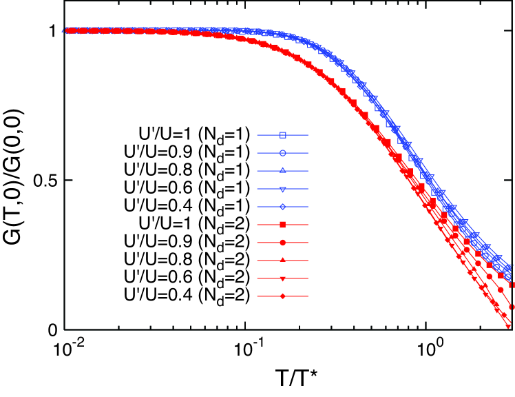
Figure 8: (color online) Universal scaling of the temperature scaled by $T^{*}$. Data are the same with Fig. 3.

We first examine a universal form of the temperature evolutions of the linear conductance

$$G(T,0)/G_{0}=F_{n}(t,0);\quad t=T/T^{*}.$$ (24)

In Fig. 8, universal temperature dependence of $G(T,0)$ either at $N_{d}=1$ or $N_{d}=2$ are confirmed numerically, by rescaling Fig. 3 as a function of $t=T/T^{*}$ with varying $U^{\prime}/U=0.4\sim 1.0$. Here we defined $T^{*}$ at each $N_{d}$ and $U^{\prime}/U$. The results are striking. For all values of $U^{\prime}/U$ both at $N_{d}=1,2$, universal curves collapse well up to $t\lesssim 1$ (an upper scale restricting the validity of the present analysis). It implies that the universal temperature dependence either at half-filling or at quarter-filling reduces to the $SU(4)$ symmetric case. Additionally Fig. 8 shows that such universal dependence differs slightly but significantly between $N_{d}=1,2$. The universal curves obtained here look very similar to those of the symmetric model $U^{\prime}=U$ obtained in NRG [32].

5.2 Universal scaling of $G(0,V)$

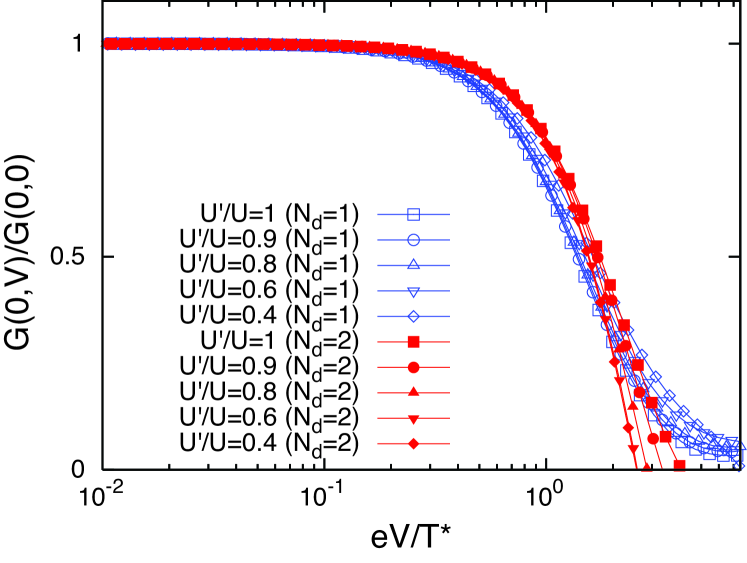
Figure 9: (color online) Universal scaling of the bias voltage scaled by $T^{*}$. Data are the same with Fig. 5.

We now turn our attention to universal scaling of non-equilibrium transport regime, of the nonlinear conductance

$$G(0,V)/G_{0}=F_{n}(0,v);\quad v=eV/T^{*}.$$ (25)

In Fig. 9, we show the bias-voltage evolution $G(0,V)$ as a function of the scaled bias voltage $v=eV/T^{*}$ either at $N_{d}=1$ or at $N_{d}=2$. As the most important observation, we can confirm that all of the universal scaling curves for $U^{\prime}/U=0.4\sim 0.9$ collapse on the $SU(4)$ symmetric one, similarly to temperature dependence. In comparing with thermal universal curves $F_{n}(t,0)$ in Fig. 8, bias-voltage universal curves $F_{n}(0,v)$ at $N_{d}=1,2$ exhibit rather similar behavior, up to $t\lesssim 1$ ($T\lesssim T^{*}$).

5.3 Universal scaling of $G(T,V)$

As a concrete dependence, thermal universal curve $F_{n}(t,0)$ and bias-voltage one $F_{n}(0,v)$ behave differently for $n=N_{d}=1,2$. This means that we need three independent variables $t$, $v$, and $n$ fully to describe a universal curve. However, a simpler description is possible to characterize the suppression by finite temperature or bias-voltage. The idea essentially comes from seeking what is a cut-off energy of the RG flow.

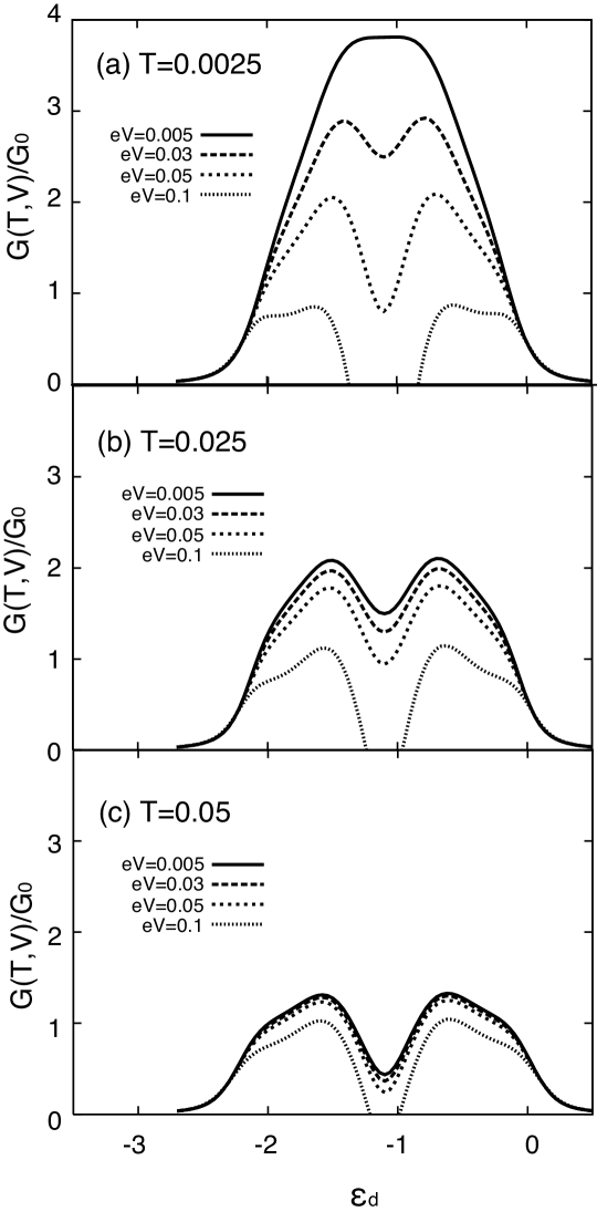
Figure 10: Conductance profiles $G(T,V)$ by varying different temperature and bias voltage. (a) $T=0.0025U$ (b) $T=0.025U$ (c) $T=0.05U$. For each temperature, results of bias voltage $eV=0.005$, $0.03$, $0.05$, and $0.1U$ are shown. The characteristic energy at half-filling is $T^{*}(2)=0.023U$.

A typical nonlinear conductance evolution at finite temperature is shown in Fig. 10 for $U^{\prime}/U=0.6$, for (a) $T=0.0025U$, (b) $0.025U$ and (c) $0.05U$. In this system, the characteristic temperature $T^{*}$ at half-filling is estimated as $T^{*}(N_{d}=2)=0.023U$. We understand its behaviors by classifying these behaviors, comparing with this energy scale $T^{*}(2)$. At (a) $T=0.0025U\ll T^{*}(2)$ ($t\ll 1$), the conductance profile looks similar to that at $T=0$ in Fig. 4 (c). It shows the temperature is so small that no thermal effect appears. On the other hand, at (c) $T=0.05U\gg T^{*}(2)$ ($t\gg 1$), all the conductance profiles with different bias-voltage $V$ almost collapse except for $eV=0.1U$ which is larger than the temperature $T=0.05U$, which is a hallmark of the temperature $T\gg T^{*}(2)$ controlling the conductance profile for a region $T\gtrsim eV$. Consistent behaviors are also confirmed at (b) $T=0.025U\approx T^{*}(2)$: the temperature controls the conductance profile for $T>eV$; the bias voltage, for $T<eV$. In Fig. 11, we illustrate universal functions $F_{n}(t,v)$ for $n=1,2$ of the $SU(4)$ universality, obtained by our KR-SBMT approach. We conclude that the larger energy scale $\max[t,v]$ between the temperature and the bias voltage effectively dominates the nonlinear conductance profile. The result presented in Fig. 11 is indeed calculated for $U^{\prime}/U=0.6$, but as we have shown so far, this universal function $F_{n}(t,v)$ is almost the same up to $T^{*}$ with that of $U^{\prime}/U=1$ and also of $U^{\prime}/U<1$.

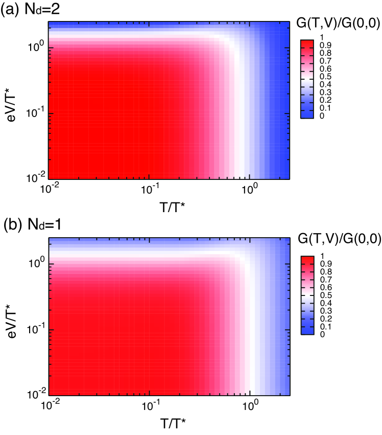
Figure 11: (color online) Universal function $F_{n}(t,v)$ of the $SU(4)$ universality class, obtained by the KR-SBMT. (a) $G(T,V)/G(0,0)=F(t,v)/4$ at half-filling ($N_{d}=2$) and (b) $G(T,V)/G(0,0)=F(t,v)/2$ at quarter-filling ($N_{d}=1$),

Before concluding this section, we give two cautionary comments regarding the applicability of the present universal dependence of the conductance: (1) on conductance profiles observed as a function of the gate voltage $\varepsilon_{d}$; (2) on the dependence on the value of $U/\Gamma$. The first point is related to our employed approximation (KR-SBMT). Although we believe the present analysis of the $T^{*}$ scaling may be useful even for $\max[T,eV]\gtrsim T^{*}$, our present KR-SBMT method is believed to describe the system adequately only up to $\lesssim T^{*}$; it does not fully incorporate charge fluctuations, which will be important for transport under a large bias. The characteristic temperature $T^{*}$ is lower at half-filing, higher at quarter-filling, particularly in the presence of the interaction asymmetry (Figs. 6, 7). Hence the conductance evaluated by the KR-SBMT is validated up to a smaller value $T$ or $eV$ at half-filling than at quarter-filling. Such signature is observed in the conductance profile for $eV=0.1U$ in Figs. 4 and 10, where $\max[T,eV]]\gg T^{*}(N_{d}=2)$ and the Coulomb blockade physics dominates the system. In those cases, the conductance is anticipated to vanish, with some nonlinear bias effect that the KR-SBMT is likely to miss. The second point is related to why our analysis observes the $SU(4)$ universality class, disregarding the interaction asymmetry, without a crossover. This important issue will be examined further in next section.

6 $T^{*}$ renormalization or a crossover: Effect of finite $U$

As we have shown, our results of conductance at finite temperature and/or bias voltage behave consistently with the $SU(4)$ universality class even in the presence of the interaction asymmetry $U^{\prime}/U<1$, exhibiting no crossover toward a different universality class. The results may seem odd at first glance, contradicting with the suggested crossover between $SU(4)$ and $SU(2)\times SU(2)$ universality classes [19]. However, such a crossover behavior takes place only for a larger value of $U/\Gamma$. In a usual range of experimentally feasible parameters, we claim the renormalization of the characteristic temperature $T^{*}$, not a crossover of the universality classes, plays a more dominant role, controlling the conductance behavior.

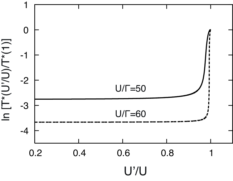
Figure 12: Dependence of the characteristic temperature $T^{*}$ on the interaction asymmetry $U^{\prime}/U$ at $N_{d}=2$ for $U/\Gamma=50$ and $60$.

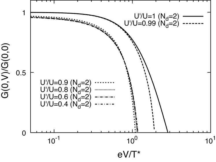
Figure 13: Universal scaling of the bias voltage scaled by $T^{*}$ at $N_{d}=2$ for $U/\Gamma=50$. A crossover between different universality classes occurs.

To support our view, we also examine the behavior with larger values of $U$. Figure 12 shows the characteristic temperature $T^{*}$ at $N_{d}=2$ as a function of the interaction asymmetry $U^{\prime}/U$ for $U/\Gamma=50,60$, to be compared with Fig. 7. In this case, the interaction asymmetry $U^{\prime}/U$ reduces $T^{*}$ quite rapidly, which signals a crossover of the universality class from $SU(4)$ to $SU(2)\times SU(2)$ [19]. We confirm that such a crossover indeed occurs by performing the universal scaling (Fig. 13). For $U/\Gamma=50$, the universal scaling indicates that the scaled curve for $U^{\prime}/U=0.9$ is clearly different from that for $U^{\prime}/U=1$ or $0.99$; the universality class crosses over between $SU(4)$ and $SU(2)\times SU(2)$ in this case.

In usual experiments, however, $U$ is roughly in the range of $U=10\sim 20\Gamma$ (see also the next section). For this case, as was shown in §5, the dominant effect at $N_{d}\approx 2$ is due to the renormalization of $T^{*}$, not a crossover of the universality classes.

7 Experimental manifestation

We have found theoretically the effect of the interaction asymmetry on the conductance profile substantial, either at finite temperature or at finite bias voltage. Currently, a few experimental realization of the $SU(4)$ Anderson model eq. (1) are known: transport through a carbon nanotube dot, and, through double quantum dots coupling capacitively with each other [3, 4]. We discuss our present results in the light of existing experimental data.

7.1 Carbon nanotube dot

Several groups have investigated and observed the Kondo enhancement in the linear conductance measurement through a carbon nanotube dot [12, 13, 14, 15]. A carbon nanotube dot has doubly degenerate orbitals in the topmost shell, and moreover, the conductance according to the $SU(4)$ Friedel sum rule eq. (20) is clearly observed experimentally at low temperatures [15]. This observation clearly justifies the validity of the $SU(4)$ Anderson model. Notwithstanding, we have not understood fully the temperature evolution of the conductance, particularly around $N_{d}\approx 2$: While the experiment by Makarovski et al. has observed visible low-temperature “Kondo-like enhancement” around $N_{d}=2$[15], such enhancement was absent exhibiting a characteristic ‘dip’ in others [13, 14]. We suggest the interaction asymmetry enables us to understand systematically finite temperature evolutions in these experiments [25].

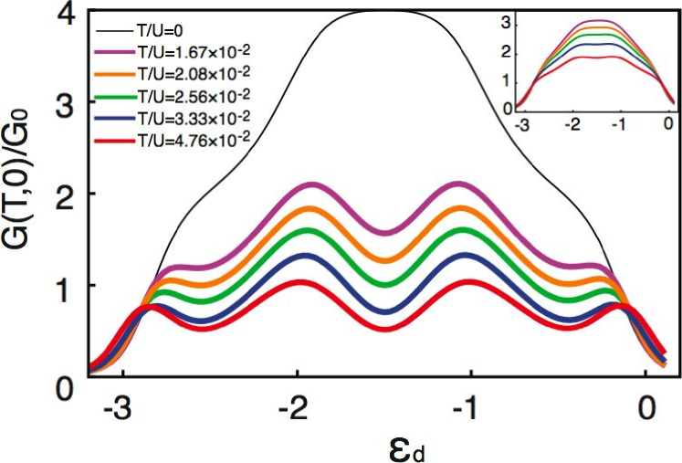
Figure 14: (color online) Schematic plotting for the comparison with carbon nanotube dot experiments: Conductance as a function of the gate voltage for $U^{\prime}/U=0.997$ and $U=30\Gamma$. $|U-U^{\prime}|\ll T^{*}(N_{d}=2,U^{\prime}=U)$ is realized. Inset shows larger coupling parameter regime $U=15\Gamma$.

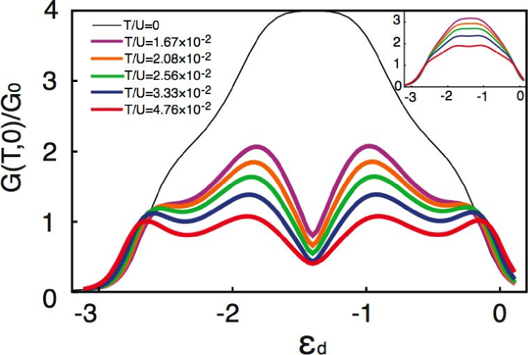
Figure 15: (color online) Schematic plotting for the comparison with carbon nanotube dot experiments: Conductance as a function of the gate voltage for $U^{\prime}/U=0.9$. Other parameters are the same with Fig. 14. $|U-U^{\prime}|\gg T^{*}(N_{d}=2,U^{\prime}=U)$ is realized.

In Figs. 14 and 15, we present schematic calculations mimicking the experimental situation, changing $U^{\prime}/U$ slightly, with $U=30\Gamma$ (with $U=15\Gamma$ for the insets). In Fig. 14 with $U^{\prime}/U=0.997$, the conductance profile reproduces all the features of the $SU(4)$ symmetric model. Notably, the Kondo enhancement at low temperature occurs either at $N_{d}\approx 2$ or at $N_{d}\approx 1$ similarly. As was claimed already in ref. Anders08, these temperature evolutions by the $SU(4)$ symmetric Anderson model agree very well with what is observed either at $V_{g}\sim 3.9\textrm{V}$ or at $V_{g}\sim 5.3\textrm{V}$ in the experiments by Makarovski et al. [15]. To our surprise, however, the conductance profiles with four peaks ($U=30\Gamma$) are modified considerably by a relatively small asymmetry (less than 10%), having a characteristic dip structure around half-filling as in Fig. 15. This is because the characteristic energy at $N_{d}=2$ is rather small, $T^{*}(N_{d}=2,U^{\prime}=U)\approx 0.014U$. The value $U^{\prime}/U=0.9$ conforms to almost equally-spaced Coulomb blockade peaks, observed at $T=8\textrm{K}$ [14]. We believe Fig. 15 captures essential characteristics experiments [13, 14] with a reasonable choice of physical parameters; for instance, in Fig. 3(a) or Fig. SI2 of Jarillo-Herreo et al.[14], the conductance at $V_{g}\approx 3\textrm{V}$ is smaller than that of $V_{g}\approx 2.8\textrm{V}$ or $3.2\textrm{V}$ at each temperature.

Regarding the mixed-valence regime ($U/\Gamma=15$, insets of Figs. 14 and 15), four peaks merge to form one big peak showing the Kondo enhancement. In this regime, we find the interaction asymmetry $U^{\prime}/U$ hardly affecting the conductance profile even at finite temperature.

7.2 Double dot system with capacitive coupling

Several groups have been investigating experimentally on orbital and/or spin Kondo effects in double quantum dot systems with capacitive coupling [3, 4, 7, 8], where the orbital Kondo effect has been observed at quarter-filling. The measured Kondo temperature is found surprisingly high. Thus we should possibly attribute the phenomena to the $SU(4)$ Kondo effect, as an entanglement of spins and orbits. Therefore, within the universality of the topmost shell, we will be able to describe the system by applying the $SU(4)$ Anderson model eq. (1).

Although the $SU(4)$ Anderson model suggests that the conductance should exhibit the Kondo enhancement both at quarter-filling and at half-filling, to the best of our knowledge, no enhancement has been observed so far at half-filling. However, we argue that the absence of the Kondo-like enhancement at half-filling is due to the combined effect of finite bias effect and the interaction asymmetry in those systems. Consequently, it is expected that the conductance enhancement should appear also at half-filling by suppressing the bias voltage at low temperature.

To make our argument more concrete, let us examine typical double dot experiments [3, 4], whose $IV$ characteristics at $T=30\textrm{mK}$ are excerpted in Fig. 16 (a), which is measured by applying the source-drain voltage $80\mu\textrm{V}$. The voltage $V_{(1-2)}$ controls the degeneracy of single levels; the topmost single orbits realize two-fold degeneracy at $V_{(1-2)}\approx 3.75,4.25,4.75,5.25$ etc. The honeycomb structure clearly shows Kondo enhancement at quarter-filling (denoting regions ‘b’ in Fig. 16(a)); no enhancement at half-filling. In Fig. 16 (b), choosing the parameters $U=0.7\textrm{meV}$, $U^{\prime}/U=0.6$, and $U/\Gamma=20$, we plot corresponding KR-SBMT results of the nonlinear conductance $G(T,V)$ by varying the source-drain voltage $V=0,35,70\,\mu\textrm{V}$. The result of $V=70\,\mu\textrm{V}$ reproduces well with experimental data; Kondo enhancement is observed at quarter-filling but not at half-filling.

Our KR-SBMT calculations evaluate the characteristic energy at half-filling $T^{*}(2)$ to be $16\mu\textrm{eV}$ for these systems. So we conclude experiments realize large bias regime suppressing the Kondo effect at $N_{d}\approx 2$. It also suggests that when we can decrease the source-drain voltage, less than $16\mu\textrm{V}$, the Kondo-like enhancement should appear at half-filling as well as at quarter-filling.

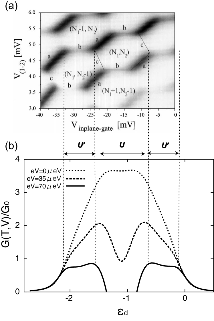
Figure 16: (a) Experimental $IV$ characteristics excerpted from refs. Wilhelm00,Wilhelm02 (see the text). (b) A schematic differential conductance obtained by the KR-SBMT at $T=30\,\textrm{mK}$, as a function of the gate voltage, varying bias voltage $V=0$, $35$, $70\,\mu\textrm{V}$.

8 Conclusion

We have investigated the role of the inter- and intra-orbital interactions in transport through quantum dots with two-fold orbital degeneracy, e.g., carbon nanotube dots, double dot systems with capacitive interaction etc. By using the $SU(4)$ Anderson model with the interaction asymmetry between orbits/dots and within the validity of the KR-SBMT, we have shown how significantly a small amount of it can affect the profile of the linear conductance at finite temperature, and of the nonlinear conductance. We have shown that the phenomena can be understood systematically by the different dependence $T^{*}$ on interaction asymmetry at each gate voltage. In addition, we have compared our theoretical results with experimental data in two typical situations: carbon nanotube dots, and double dot systems with capacitive interaction. We believe our theoretical results agree very well, suggesting unexplored phenomena of the Kondo enhancement in double dot systems. We have shown clearly the interaction asymmetry is essential in explaining conductance profiles through these two-fold degenerate systems in real experiments.

9 Acknowledgments

The authors appreciate K. Isozaki, W. Izumida and H. Tamura for helpful discussion. One of the authors (H.O.) thanks S. Okada and K. Shiraishi for their support. The work was partially supported by Grant-in-Aid for Scientific Research (Grant No. 18063003 and 18500033) from the Ministry of Education, Culture, Sports, Science and Technology of Japan and the Core Research for Evolutional Science and Technology from Japan Science and Technology Corporation.

References

- [1] D. Goldhaber-Gordon, H. Shtrikman, D. Mahalu, D. Abusch-Magder, U. Meirav, and M. A. Kastner: Nature 391 (1998) 156.
- [2] U. Wilhelm, J. Schmid, J. Weis, and K. v. Klitzing: Physica E9 (2001) 625.
- [3] U. Wilhelm and J. Weis: Physica E6 (2000) 668.
- [4] U. Wilhelm, J. Schmid, J. Weis, and K. v. Klitzing: Physica E14 (2002) 385.
- [5] I. H. Chan, R. M. Westervelt, K. D. Maranowski, and A. C. Gossard: Applied Phys. Lett. 80 (2002) 1818.
- [6] D. T. McClure, L. DiCarlo, Y. Zhang, H.-A. Engel, and C. M. Marcus: Phys. Rev. Lett. 98 (2007) 056801.
- [7] A. Hübel, J. Weis, W. Dietsche, and K. v. Klitzing: Applied Phys. Lett. 91 (2007) 102101.
- [8] A. Hübel, K. Held, J. Weis, and K. v. Klitzing: Phys. Rev. Lett. 101 (2008) 186804.
- [9] T. Pohjola, H. Schoeller, and G. Schön: Europhys. Lett. 54 (2001) 241.
- [10] D. Boese, W. Hofstetter, and H. Schoeller: Phys. Rev. B 66 (2002) 125315.
- [11] S. Sasaki, S. D. Franceschi, J. M. Elzerman, W. G. van der Wiel, M. Eto, S. Tarucha, and L. P. Kouwenhoven: Nature 405 (2000) 764.
- [12] J. Nygard, D. H. Cobden, and P. E. Lindelof: Nature 408 (2000) 342.
- [13] B. Babić, T. Kontos, and C. Schönenberger: Phys. Rev. B 70 (2004) 235419.
- [14] P. Jarillo-Herrero, J. Kong, H. S. J. van der Zant, C. Dekker, L. P. Kouwenhoven, and S. D. Franceschi: Nature 434 (2005) 484.
- [15] A. Makarovski, J. Liu, and G. Finkelstein: Phys. Rev. Lett. 99 (2007) 066801.
- [16] L. Borda, G. Zaránd, W. Hofstetter, B. I. Halperin, and J. von Delft: Phys. Rev. Lett. 90 (2003) 026602.
- [17] M.-S. Choi, R. López, and R. Aguado: Phys. Rev. Lett. 95 (2005) 067204.
- [18] J. S. Lim, M.-S. Choi, M. Y. Choi, R. López, and R. Aguado: Phys. Rev. B 74 (2006) 205119.
- [19] M. R. Galpin, D. E. Logan, and H. R. Krishnamurthy: Phys. Rev. Lett. 94 (2005) 186406.
- [20] M. R. Galpin, D. E. Logan, and H. R. Krishnamurthy: J. Phys.: Condens. Matter 18 (2006) 6545.
- [21] M. Eto and Y. V. Nazarov: Phys. Rev. Lett. 85 (2000) 1306.
- [22] D. Goldhaber-Gordon, J. Göres, M. A. Kastner, H. Shtrikman, D. Mahalu, and U. Meirav: Phys. Rev. Lett. 81 (1998) 5225.
- [23] M. Grobis, I. G. Rau, R. M. Potok, H. Shtrikman, and D. Goldhaber-Gordon: Phys. Rev. Lett. 100 (2008) 246601.
- [24] J. Rincón, A. A. Aligia, and K. Hallberg: Phys. Rev. B 79 (2009) 121301R.
- [25] H. Oguchi and N. Taniguchi: J. Phys. Soc. Jpn 78 (2009) 083711.
- [26] G. Kotliar and A. E. Ruckenstein: Phys. Rev. Lett. 57 (1986) 1362.
- [27] We here extend the original KR formulation, which breaks the spin-rotational symmetry. The approach can be formulated in a spin-rotational invariant way (see T. Li, P. Wölfle, and P. J. Hirschfeld: Phys. Rev. B 40 (1989) 6817), but it does not affect the mean field result.
- [28] B. Dong and X. L. Lei: J. Phys.: Condens. Matter 13 (2001) 9245.
- [29] J. Takahashi and S. Tasaki: J. Phys. Soc. Japan 75 (2006) 094712.
- [30] B. Dong and X. L. Lei: Phys. Rev. B 66 (2002) 113310.
- [31] N. S. Wingreen and Y. Meir: Phys. Rev. B 49 (1994) 11040.
- [32] F. B. Anders, D. E. Logan, M. R. Galpin, and G. Finkelstein: Phys. Rev. Lett. 100 (2008) 086809.
- [33] This is believed to be an artifact of the Gutzwiller approximation, to which the KR-SBMT reduces at .
- [34] C. Karrasch, T. Enss, and V. Meden: Phys. Rev. B 73 (2006) 235337.
- [35] A. K. Mitchell, M. R. Galpin, and D. E. Logan: Europhys. Lett. 76 (2006) 95.
- [36] C. A. Büsser and G. B. Martins: Phys. Rev. B 75 (2007) 045406.