Initial phases of massive star formation in high infrared extinction clouds.

Abstract

Aims. The earliest phases of massive star formation are found in cold and dense infrared dark clouds (IRDCs). Since the detection method of IRDCs is very sensitive to the local properties of the background emission, we present here an alternative method to search for high column density in the Galactic plane by using infrared extinction maps. Using this method we find clouds between 1 and 5 kpc, of which many were missed by previous surveys. By studying the physical conditions of a subsample of these clouds, we aim at a better understanding of the initial conditions of massive star formation.

Methods. We have made extinction maps of the Galactic plane based on the $3.6-4.5$ $\mu$m color excess between the two shortest wavelength Spitzer IRAC bands, reaching to visual extinctions of $\sim$100 mag and column densities of $9\times 10^{22}\leavevmode\nobreak\ \mathrm{cm^{-2}}$. From this we compiled a new sample of cold and compact high extinction clouds. We used the MAMBO array at the IRAM 30m telescope to study the morphology, masses and densities of the clouds and the dense clumps within them. The latter were followed up by pointed ammonia observations with the 100m Effelsberg telescope, to determine rotational temperatures and kinematic distances.

Results. Extinction maps of the Galactic plane trace large scale structures such as the spiral arms. The extinction method probes lower column densities, $N_{\mathrm{H_{2}}}\sim 4\times 10^{22}\,\mathrm{cm^{-2}}$, than the 1.2 mm continuum, which reaches up to $N_{\mathrm{H_{2}}}\sim 3\times 10^{23}\,\mathrm{cm^{-2}}$ but is less sensitive to large scale structures. The 1.2 mm emission maps reveal that the high extinction clouds contain extended cold dust emission, from filamentary structures to still diffuse clouds. Most of the clouds are dark in 24 $\mu$m, but several show already signs of star formation via maser emission or bright infrared sources, suggesting that the high extinction clouds contain a variety of evolutionary stages. The observations suggest an evolutionary scheme from dark, cold and diffuse clouds, to clouds with a stronger 1.2 mm peak and to finally clouds with many strong 1.2 mm peaks, which are also warmer, more turbulent and already have some star formation signposts.

1 Introduction

Massive stars play a fundamental role in the evolution of galaxies through their strong UV radiation, stellar winds and supernovae explosions, which contribute to the chemical enrichment of the interstellar medium. Massive stars are rare, hence usually found at large distances. They form very rapidly while still deeply embedded in their natal molecular clouds. These characteristics impose several observational obstacles, like the necessity of high resolution and sensitivity in an un-absorbed frequency range, to study their formation.

Currently, the earliest stage of massive star formation is thought to take place in the very dense clumps found in Infrared Dark Clouds (IRDCs). The properties of IRDCs are shown by Carey et al. (1998) to be dense ($n_{\mathrm{gas}}>10^{5}\,\mathrm{cm^{-3}}$) and cool ($T<20\,\mathrm{K}$) aggregations of gas and dust in the Galaxy. They contain clumps with typical masses of $\geq 100\,\mathrm{M_{\odot}}$ (Rathborne et al., 2006; Pillai et al., 2006; Simon et al., 2006b). From IRDC clumps to the next stage, the high-mass protostellar objects (HMPOs, Beuther et al., 2002; Sridharan et al., 2002), the temperatures increase ($30\,\mathrm{K}<\mathrm{T}<60\,\mathrm{K}$), the line widths increase, densities and masses rise (Motte et al., 2007). HMPOs are usually found prior to the formation of ultra compact Hii (UCHii) regions, before the newly formed star begins to ionize its surrounding medium.

Motte et al. (2007) demonstrated the difficulty of finding massive objects in an early evolutionary phase: in their survey of 3 deg² in Cygnus X, they found little evidence for dense clumps without any trace of star formation, however dense clumps with already ongoing star formation were found to be abundantly present. Based on these results, the statistical life time of the high-mass protostars and prestellar cores was estimated $\leq 3\times 10^{4}$ yr (Motte et al., 2007), which is much shorter than what is found in nearby low-mass star-forming regions: $\sim$$3\times 10^{5}$ yr (Kirk et al., 2005). It is these very early stages, which provide important clues to construct a theoretical model of massive star formation, since the initial fragmentation of the gas and dust in a clump will be different in the case of monolithical collapse (Krumholz et al., 2009) compared to the competitive accretion model (Bonnell et al., 2001; Clark et al., 2008).

Massive stars generally form in clusters (Lada & Lada, 2003), of which the precursors are massive clumps or the so-called precluster forming clumps, hereafter just clumps, of a $\sim$1 pc size. For many massive star-forming regions, we do not yet have the capacity to resolve the clumps into prestellar cores and study the fragmentation (Beuther et al., 2007; Rathborne et al., 2007, 2008; Zhang et al., 2009; Swift, 2009). In this paper, we report on the physical parameters of the clumps, such as their morphology, density and temperature. Based on this, we hypothesize on an evolutionary sequence of cluster formation.

Our understanding of the clumps increased considerably with the discovery of IRDCs. IRDCs are detected by a local absence of infrared (IR) emission against the diffuse mid IR emission of the Galactic plane (Perault et al., 1996; Egan et al., 1998) and are observed numerously throughout the Milky Way (Simon et al., 2006b). At the typical low temperatures of IRDCs ($\sim 20$ K), the dust emission peaks in the far-infrared and is optically thin at mm/submm wavelengths. For a majority of IRDCs the mm dust emission coincides with the morphology of the IR absorption (Rathborne et al., 2006; Pillai et al., 2006). Many clumps in IRDCs show signs of star formation via infrared emission at 24 $\mu$m, or SiO emission from shocks driven by outflows (Motte et al., 2007; Beuther & Sridharan, 2007; Chambers et al., 2009). Observations tell that clumps in IRDCs span a very wide range of masses, indicating that not all will form clusters with massive stars (Rathborne et al., 2006; Pillai et al., 2006).

The detection method of IRDCs is very sensitive to the local properties of the background emission. Also, not all massive dust condensations will be infrared dark if there is enough foreground emission. Hence, to find the high mass end of molecular clouds in an unbiased fashion, new, complementary approaches are needed. We have developed such a new method, well known from studies of low mass star-forming regions, to target more efficiently the most massive clouds: Lada et al. (1994) pioneered the method of measuring high amounts of extinction through stellar color excess in the infrared. Applied to the 2 $\mu$m data of the 2MASS survey, they covered the range up to 40 magnitudes in visual extinction, $A_{V}$. However, this is not sufficient to probe the dense birthplaces of massive stars. Here the results of the Spitzer Space Telescope GLIMPSE survey (Benjamin et al., 2003) came to help: by applying the extinction curve of Indebetouw et al. (2005) we have extended the color excess method to reach up to peaks in $A_{V}$ of $\sim$100 magnitudes (or column densities $N_{\mathrm{H_{2}}}$ of $9\times 10^{22}$ cm^-2), thus entering the realm where massive star formation becomes possible. The extinction method, however, is limited by the number of available background stars, and will therefore detect mainly nearby clouds (discussed in Sect. 2.1). In the meanwhile, complementary, unbiased dust continuum surveys were carried out: the ATLASGAL survey of the complete inner Galactic plane at 870 $\mu$m by Schuller et al. (2009) and the 1.1 mm BOLOCAM survey (Rosolowsky et al., 2009) of the Galactic plane accessible from the northern hemisphere.

We selected the more compact and high extinction (mean $A_{\mathrm{V}}>20\,\mathrm{mag}$ or $N_{\mathrm{H_{2}}}>2\times 10^{22}$ cm^-2) sources from large scale extinction maps of the inner Galactic plane ($-60\degr<l<60\degr$, $0.9\degr<b<-0.9\degr$). These high extinction clouds (HECs) were studied in the millimeter dust continuum and the rotational transitions of ammonia ($\mathrm{NH_{3}}$). $\mathrm{NH_{3}}$ has proven to be a reliable tracer of dense gas in dark clouds: not only does the $\mathrm{NH_{3}}$ emission match the submillimeter dust emission peaks (Pillai et al., 2006), but also do observations show that, unlike other molecules, $\mathrm{NH_{3}}$ does not deplete from the gas phase for typical IRDC densities – Pagani et al. (2005) observed that $\mathrm{NH_{3}}$ depletes at densities of $10^{6}\,\mathrm{cm^{-3}}$ in agreement with the prediction of Bergin & Langer (1997). Moreover, throughout the evolutionary stages of massive star formation, $\mathrm{NH_{3}}$ shows an increasing trend in averaged line widths and temperatures from less to more evolved sources (Pillai et al., 2006), which indicates that the $\mathrm{NH_{3}}$ molecule is also a tracer of evolutionary phase.

This study presents an overview from the high extinction complexes on Galactic size-scales, covering several tens of parsecs, to the clumps found in the 1.2 mm continuum of $0.1-0.7$ pc in size. The connection between the largest and smallest scale is important for a comprehensive view of cluster formation in giant molecular clouds. In section 2 , we present the method of extinction mapping. Observations and data reduction are described in section 3, and the results follow in section 4. The analysis and discussion of the physical parameters are given in section 5, and are compared to previous studies and theoretical predictions in section 6.

2 High extinction clouds

2.1 Method: extinction mapping

The overall distribution of dust in a cloud can be traced by the extinction of background starlight at visual and near-infrared wavelengths as it passes through a cloud (Lada et al., 1994). Since extinction decreases with wavelength, observations at longer wavelengths probe deeper into the cloud and trace denser regions. Additionally the number of detectable background stars increases at these wavelengths. With the advance of infrared cameras it became possible to detect several hundreds of background stars through a cloud, allowing to convert the infrared images covering them in extinction maps of useful resolution.

The GLIMPSE survey employed the Infrared Array Cameras (Fazio et al., 2004) onboard the Spitzer Space telescope, operating at 3.6, 4.5, 5.8 and 8.0 $\mu$m. We used the data provided by the GLIMPSE I survey (release April 2005), which covered longitudes of $l=10-65\degr,\leavevmode\nobreak\ 295-350\degr$ with $b=\pm 1\degr$. The calibration of the data is described in Reach et al. (2005). The inner 20° of the Galactic Plane, except for the innermost $\pm 1\degr$, was taken from the GLIMPSE II survey (2007).

To construct the extinction maps we used the averaged (3.6 $\mu$m–4.5 $\mu$m) color excess, because the extinction law determination for these wavelengths is the most accurate of all the Spitzer bands. The averaged color excess, $<E(3.6\,\mu\mathrm{m}-4.5\,\mu\mathrm{m})>$, was calculated from the color excess in a large scale field (a box of size $108\arcsec\times 108\arcsec$):

$$<E(3.6\,\mu\mathrm{m}-4.5\,\mu\mathrm{m})>=\hskip 110.96556pt$$

$$<(3.6\,\mu\mathrm{m}-4.5\,\mu\mathrm{m})-(3.6\,\mu\mathrm{m}-4.5\,\mu\mathrm{m})_{0}>\,,$$ (1)

where the background stars are taken to be common-type K giants. Measurements of $(3.6\,\mu\mathrm{m}-4.5\,\mu\mathrm{m})_{0}$ in such control fields showed that K giants have an average color of $\sim$0 mag with a dispersion of 0.2 mag. Starting from the reddening law for $<E(H-K)>$ in Lada et al. (1994), one can extend it following Indebetouw et al. (2005), and get the relation between the averaged color excess to the averaged visual extinction, $<A_{V}>$:

$$<A_{V}>=81.8<E(3.6\,\mu\mathrm{m}-4.5\,\mu\mathrm{m})>\hskip 14.22636pt[\mathrm{mag}].$$ (2)

The color excess map can be contaminated by embedded stars in the cloud itself or by foreground stars. The latter will increase in number as the cloud is located at a farther distance. Since the foreground stars will not be reddened, they decrease the average color excess of the field. For example, if the number of foreground stars equals the number of background stars the color excess will be halved. It also means that for far away clouds the color excess will be underestimated. Rathborne et al. (2006) and Chambers et al. (2009) find signs of active massive star formation in one of our clouds. Such young red objects will contribute to the measured color excess, which will lead to an overestimation of the derived extinction. However, the selection of clouds associated with very early phases of star formation will not be affected.

In general, the limits of extinction mapping are set by the number of available background stars; their number has to be sufficient for a statistically meaningful color excess determination. Thus, the reach of the extinction method will change with Galactic latitude, because at higher latitudes the number of stars decreases. In the Galactic plane, there will be “horizon” to which one can measure a sufficient color excess, however this horizon will be far from uniform; it depends for every direction on the number of K giants in front and behind the clouds, which will differ when crossing a spiral arm or moving in toward the Galactic center.

Recently, Chapman et al. (2009) studied the changes in the mid-infrared extinction law within a large region with high resolution. They find that while in regions with a K-band extinction of $A_{\mathrm{K}}\leq 0.5$ mag the extinction law is well fitted by an extinction factor of $R_{\mathrm{V}}=3.1$ (Weingartner & Draine, 2001), the regions with $A_{\mathrm{K}}\geq 1.0$ mag are more consistent with the Weingartner & Draine (2001) model of $R_{\mathrm{V}}=5.5$, which uses larger maximum dust grain sizes. The high extinction clouds are by definition very dense regions for which $A_{\mathrm{K}}>1.0$ mag. This means that the visual extinctions and column densities reached by the extinction mapping are a factor $\sim$1.8 higher than estimated from Eq. 2, where we used $R_{\mathrm{V}}=3.1$. The near and mid-infrared extinction law is of great interest, and recently many publications appeared on the mid-infrared (Flaherty et al., 2007; Nishiyama et al., 2009; Zasowski et al., 2009) and the near-infrared (Moore et al., 2005; Froebrich & del Burgo, 2006; Stead & Hoare, 2009) extinction law. Within the range of 3.6 and 4.5 $\mu$m, the range we used for our extinction maps, there is a reasonable agreement between the results of Indebetouw et al. (2005) and most recent studies.

2.2 Catalog of high extinction clouds

We made extinction maps for the complete inner part of the Galaxy with a resolution of 108″, plotted in Fig. 1. The mid-infrared extinction is changing with longitude and latitude, because it is sensitive to large-scale structures. Fig. 2 shows histograms of the average color excess in longitude and latitude. Most of the peaks in the color excess can be associated to Galactic spiral arms. The large-scale structure of the extinction was excluded by selecting only compact high extinction regions with an color excess above 0.25 mag (equivalent to a hydrogen column density of $2\times 10^{22}$ cm^-2). In a second step, smaller extinction maps with a higher resolution ($54\arcsec$) were computed to obtain more accurate positions of the highest extinction peaks. These peaks were selected by eye. Regions with known sources, such as Hii regions and HMPOs, were discarded, leaving a sample of unknown and possibly cold and massive clouds. In this paper we studied 25 high extinction clouds (HECs) in the first Galactic quadrant. These were the clouds, visible from the northern hemisphere, with the highest extinction peaks which were not associated with Hii regions from the Becker et al. (1994) survey and which had no available mm/submm maps from the literature. A complete catalog of all the high extinction clouds is given in Table LABEL:ta:ext, where for each cloud the center position in J2000 coordinates is listed with its corresponding peak color excess.

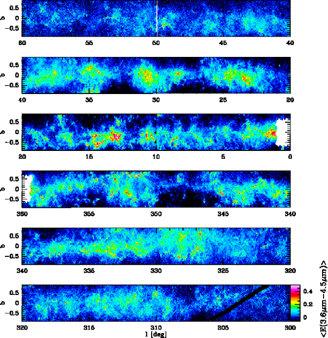
Figure 1: The color excess $\mathrm{<E(3.6\mu\mathrm{m}-4.5\mu\mathrm{m})>}$ for the first (top three graphs) and fourth (bottom three graphs) quadrant of the Galaxy. The extinction maps are available in fits format on the CDS.

1

Table 1: Catalog of high extinction clouds (HECs) with the peak color excess, $E<(3.6\,\mu\mathrm{m}-4.5\,\mu\mathrm{m})>$

HEC name	R.A.	Dec.	Color Excess	HEC name	R.A.	Dec.	Color Excess
	(h:m:s)	(°: ′: ″)	(mag)		(h:m:s)	(°: ′: ″)	(mag)
	(J2000)	(J2000)			(J2000)	(J2000)
1st quadrant clouds				4th quadrant clouds
G011.09–00.54	18:12:01.2	–19:36:07	0.40	G313.26–00.72	14:20:34.2	–61:47:42	0.48
G012.54–00.35	18:14:15.8	–18:14:11	0.29	G313.72–00.29	14:22:57.1	–61:13:49	0.69
G012.65–00.17	18:13:49.6	–18:02:53	0.45	G314.21+00.21	14:25:18.8	–60:35:22	0.70
G012.73–00.58	18:15:33.2	–18:08:45	0.29	G314.27+00.09	14:26:07.4	–60:40:48	0.67
G012.89+00.48	18:11:52.7	–17:31:27	0.55	G314.31+00.12	14:26:21.3	–60:38:31	0.58
G013.28–00.34	18:15:40.8	–17:34:32	0.57	G316.45–00.63	14:44:46.4	–60:29:47	0.47
G013.38–00.27	18:15:38.8	–17:27:26	0.47	G316.73+00.06	14:44:28.6	–59:45:12	0.49
G013.91–00.51	18:17:34.8	–17:06:07	0.58	G316.77–00.02	14:45:02.6	–59:48:25	0.89
G013.97–00.45	18:17:27.6	–17:01:34	0.51	G317.70+00.11	14:51:11.0	–59:16:52	0.53
G014.33–00.65	18:18:55.4	–16:48:12	0.53	G317.88–00.26	14:53:46.2	–59:31:40	0.89
G014.39–00.75	18:19:24.1	–16:47:34	0.42	G318.05+00.09	14:53:43.9	–59:08:36	0.90
G014.45–00.09	18:17:06.1	–16:25:37	0.50	G318.78–00.17	14:59:40.2	–59:02:11	0.84
G014.63–00.57	18:19:13.6	–16:29:56	0.57	G320.19+00.85	15:05:20.9	–57:28:03	0.76
G014.72–00.21	18:18:04.7	–16:14:47	0.46	G321.93–00.01	15:19:42.4	–57:18:40	1.06
G015.09–00.60	18:20:14.0	–16:06:38	0.33	G322.16+00.64	15:18:33.9	–56:38:03	0.67
G015.21–00.62	18:20:33.2	–16:00:37	0.40	G323.19+00.15	15:26:47.7	–56:29:15	0.64
G015.51–00.42	18:20:23.8	–15:39:22	0.31	G323.72–00.28	15:31:44.6	–56:32:20	0.52
G016.33–00.55	18:22:27.7	–14:59:20	0.31	G325.51+00.42	15:39:08.4	–54:55:47	0.57
G016.37–00.21	18:21:18.7	–14:48:01	0.36	G326.40+00.93	15:41:58.5	–53:59:04	0.86
G016.54–00.39	18:22:19.1	–14:43:50	0.28	G326.47+00.70	15:43:16.2	–54:07:35	0.80
G016.81–00.33	18:22:35.9	–14:27:46	0.30	G326.47+00.88	15:42:29.3	–53:59:03	0.95
G016.93+00.24	18:20:46.0	–14:05:28	0.30	G326.62+00.61	15:44:26.9	–54:06:02	0.95
G017.19+00.81	18:19:12.9	–13:35:18	0.37	G326.77–00.12	15:48:22.3	–54:35:29	0.85
G018.11–00.30	18:25:00.0	–13:18:15	0.26	G326.80+00.37	15:46:24.8	–54:10:57	0.67
G018.15–00.39	18:25:24.8	–13:18:34	0.28	G326.95–00.16	15:49:30.7	–54:30:42	0.44
G018.26–00.24	18:25:05.3	–13:08:26	0.40	G326.97–00.02	15:49:01.0	–54:23:15	0.77
G018.48–00.18	18:25:16.9	–12:54:56	0.26	G327.16–00.24	15:50:59.1	–54:26:28	0.46
G018.63–00.06	18:25:09.3	–12:43:43	0.29	G327.29–00.58	15:53:05.3	–54:37:13	0.46
G018.84–00.49	18:27:05.1	–12:44:30	0.29	G327.40–00.41	15:52:57.9	–54:25:05	0.68
G018.87–00.42	18:26:54.1	–12:41:05	0.27	G327.85–00.56	15:56:01.5	–54:15:02	0.53
G018.99–00.03	18:25:42.8	–12:23:51	0.48	G328.06+00.38	15:53:02.6	–53:23:27	0.55
G019.29+00.06	18:25:56.6	–12:05:11	0.32	G328.11+00.61	15:52:20.6	–53:11:00	0.46
G019.37–00.03	18:26:26.1	–12:03:31	0.36	G328.26–00.53	15:58:01.3	–53:57:44	0.56
G019.62–00.66	18:29:12.2	–12:07:52	0.30	G328.81+00.64	15:55:46.8	–52:43:01	0.80
G019.89–00.54	18:29:16.5	–11:50:27	0.27	G329.03–00.20	16:00:30.6	–53:12:37	0.93
G019.91–00.79	18:30:14.3	–11:56:07	0.25	G329.06–00.30	16:01:06.9	–53:16:05	0.67
G020.10–00.70	18:30:14.1	–11:43:18	0.26	G329.46+00.51	15:59:38.0	–52:23:28	0.60
G022.06+00.21	18:30:40.5	–09:34:11	0.35	G329.72+00.81	15:59:37.6	–51:59:53	0.60
G022.57–00.02	18:32:25.6	–09:13:08	0.26	G330.78+00.25	16:07:09.3	–51:42:48	1.01
G022.85–00.45	18:34:30.3	–09:10:11	0.28	G330.87–00.37	16:10:17.6	–52:06:33	1.10
G022.96+00.03	18:32:59.5	–08:51:08	0.26	G330.99+00.34	16:07:45.7	–51:30:39	0.55
G022.98–00.19	18:33:49.6	–08:55:50	0.26	G331.25–00.44	16:12:23.9	–51:53:57	0.49
G023.09–00.15	18:33:53.3	–08:49:05	0.30	G331.38+00.15	16:10:27.1	–51:23:04	0.55
G023.25–00.36	18:34:54.9	–08:46:36	0.32	G331.41–00.36	16:12:48.9	–51:44:25	0.64
G023.29–00.06	18:33:56.7	–08:36:09	0.35	G331.53–00.08	16:12:09.7	–51:27:08	0.50
G023.35–00.21	18:34:34.5	–08:37:04	0.35	G331.63+00.53	16:09:58.6	–50:56:03	0.48
G023.38–00.12	18:34:19.2	–08:32:53	0.41	G331.71+00.59	16:10:04.2	–50:50:23	0.73
G023.44–00.06	18:34:13.1	–08:27:47	0.31	G332.15+00.05	16:14:26.3	–50:55:29	0.50
G023.45–00.51	18:35:52.4	–08:39:48	0.28	G332.19–00.02	16:14:58.1	–50:56:49	0.43
G023.47+00.09	18:33:43.9	–08:22:18	0.27	G333.02+00.76	16:15:20.8	–49:48:32	0.50
G023.57+00.12	18:33:48.9	–08:16:00	0.26	G333.08–00.56	16:21:22.0	–50:42:51	0.59
G024.02+00.14	18:34:34.9	–07:51:38	0.26	G333.19–00.09	16:19:47.5	–50:18:26	0.56
G024.07+00.18	18:34:32.8	–07:47:49	0.28	G333.20–00.36	16:21:03.0	–50:29:19	0.43
G024.18+00.03	18:35:17.0	–07:46:11	0.27	G333.22–00.41	16:21:19.3	–50:30:37	0.46
G024.37–00.15	18:36:16.5	–07:40:56	0.32	G333.31–00.36	16:21:32.2	–50:24:41	0.51
G024.43–00.24	18:36:42.2	–07:40:06	0.31	G333.47–00.15	16:21:18.9	–50:08:51	0.44
G024.50+00.09	18:35:39.2	–07:27:13	0.27	G333.49–00.24	16:21:46.8	–50:12:19	0.57
G024.61–00.33	18:37:21.6	–07:33:08	0.31	G333.60–00.22	16:22:09.9	–50:06:32	0.44
G024.64+00.15	18:35:41.4	–07:18:22	0.38	G333.66+00.37	16:19:50.9	–49:38:47	0.68
G024.82–00.11	18:36:57.6	–07:16:02	0.26	G333.75–00.33	16:23:17.6	–50:04:46	0.56
G024.94–00.15	18:37:19.4	–07:10:34	0.35	G333.76+00.35	16:20:25.0	–49:35:26	0.54
G025.15–00.28	18:38:09.6	–07:02:52	0.32	G334.20–00.20	16:24:42.2	–49:39:56	0.43
G025.63–00.12	18:38:30.1	–06:32:55	0.32	G334.45–00.24	16:25:58.1	–49:31:03	0.50
G025.79+00.81	18:35:26.6	–05:58:57	0.19	G335.06–00.42	16:29:22.5	–49:11:57	0.77
G028.53+00.21	18:42:39.1	–03:49:20	0.30	G335.25–00.30	16:29:38.2	–48:59:04	0.68
G030.48–00.38	18:48:20.1	–02:21:16	0.29	G335.28–00.13	16:29:00.9	–48:50:43	0.69
G030.62+00.18	18:46:34.4	–01:58:31	0.31	G335.44–00.23	16:30:07.0	–48:47:56	0.82
G030.73+00.12	18:47:00.0	–01:54:22	0.32	G337.15–00.39	16:37:46.4	–47:38:49	0.79
G030.90+00.00	18:47:43.1	–01:48:24	0.30	G337.45–00.40	16:39:00.2	–47:26:07	0.45
G031.05+00.27	18:47:02.7	–01:33:08	0.30	G337.50–00.19	16:38:18.9	–47:15:09	0.48
G034.03–00.33	18:54:36.9	+00:49:43	0.30	G337.77–00.34	16:40:00.7	–47:08:50	0.53
G034.11+00.06	18:53:22.0	+01:04:37	0.30	G337.93–00.51	16:41:23.3	–47:08:51	0.64
G034.34–00.90	18:57:12.8	+00:50:40	0.30	G339.26–00.41	16:46:01.8	–46:04:40	0.53
G034.35–00.72	18:56:35.7	+00:56:11	0.34	G339.58–00.13	16:46:00.1	–45:38:54	0.52
G034.71–00.63	18:56:55.6	+01:17:44	0.41	G339.62–00.12	16:46:05.1	–45:37:07	0.41
G034.77–00.81	18:57:40.0	+01:15:57	0.39	G340.06–00.24	16:48:14.9	–45:21:32	0.47
G034.85+00.43	18:53:23.6	+01:54:07	0.34	G340.26–00.24	16:48:59.8	–45:12:03	0.57
G034.98+00.30	18:54:06.3	+01:57:43	0.31	G340.77–00.12	16:50:18.0	–44:44:05	0.44
G035.19–00.75	18:58:13.9	+01:40:07	0.59	G340.93–00.23	16:51:21.4	–44:40:36	0.61
G035.49–00.30	18:57:10.4	+02:08:27	0.38	G341.12–00.42	16:52:51.9	–44:39:26	0.60
G036.42–00.15	18:58:20.4	+03:02:04	0.27	G341.12–00.42	16:52:51.6	–44:39:17	0.61
G037.26+00.09	18:59:01.9	+03:53:40	0.36	G341.21–00.24	16:52:25.3	–44:28:11	0.47
G037.44+00.14	18:59:09.6	+04:04:18	0.28	G342.57+00.18	16:55:21.5	–43:09:13	0.56
G037.48+00.07	18:59:29.3	+04:05:03	0.29	G343.40–00.33	17:00:21.5	–42:49:13	0.52
G037.54+00.20	18:59:08.7	+04:11:44	0.29	G343.75–00.16	17:00:48.1	–42:26:19	0.56
G037.65+00.12	18:59:38.5	+04:15:22	0.29	G343.76–00.15	17:00:49.1	–42:25:24	0.56
G038.93–00.36	19:03:40.9	+05:10:19	0.48	G343.84–00.08	17:00:45.1	–42:19:04	0.66
G044.30+00.03	19:12:17.0	+10:07:02	0.31	G344.10–00.65	17:04:03.9	–42:27:36	0.81
G046.33–00.24	19:17:05.9	+11:47:23	0.32	G344.21–00.61	17:04:14.8	–42:21:09	0.44
G048.90–00.27	19:22:08.9	+14:02:57	0.41	G344.99–00.23	17:05:10.4	–41:29:38	0.87
G049.39–00.31	19:23:16.0	+14:27:17	0.34	G345.00–00.23	17:05:12.5	–41:29:35	0.50
G049.48–00.38	19:23:40.6	+14:30:25	0.60	G345.04–00.21	17:05:15.2	–41:26:59	1.20
G050.06+00.06	19:23:13.0	+15:13:28	0.36	G345.26–00.04	17:05:14.5	–41:10:16	0.80
G050.39–00.41	19:25:34.4	+15:17:32	0.35	G345.49+00.31	17:04:29.1	–40:46:27	0.64
G053.14+00.07	19:29:18.0	+17:56:08	0.46	G345.50+00.34	17:04:24.5	–40:44:38	1.21
G053.21–00.09	19:30:01.7	+17:55:28	0.34	G345.67+00.34	17:04:58.5	–40:36:44	0.82
G053.24+00.06	19:29:31.8	+18:01:14	0.57	G348.18+00.47	17:12:10.4	–38:31:19	0.95
G053.57+00.06	19:30:12.6	+18:18:35	0.37	G350.02–00.51	17:21:39.5	–37:35:45	0.95
G053.63+00.03	19:30:26.3	+18:20:40	0.33	G350.52–00.36	17:22:27.3	- -37:05:32	0.79
G053.81–00.00	19:30:54.4	+18:29:32	0.41	G350.69–00.48	17:23:26.9	–37:01:05	0.52
G058.48+00.42	19:39:01.4	+22:46:46	0.30	G350.94+00.75	17:19:06.7	–36:07:04	0.45
G059.63–00.18	19:43:47.6	+23:28:45	0.30	G350.94+00.66	17:19:30.2	–36:09:52	0.83
G059.79+00.06	19:43:13.2	+23:44:22	0.29	G350.96+00.55	17:19:58.7	–36:12:56	0.57
4th quadrant clouds				G351.16+00.71	17:19:53.7	–35:57:29	0.62
G300.91+00.88	12:34:13.0	–61:55:39	1.00	G351.25+00.66	17:20:23.3	–35:54:39	0.82
G305.36+00.19	13:12:33.8	–62:35:12	0.58	G351.44+00.66	17:20:54.7	–35:45:11	0.92
G309.13–00.14	13:45:14.1	–62:21:36	0.52	G351.47–00.45	17:25:30.5	–36:21:33	0.75
G309.37–00.12	13:47:18.1	–62:17:35	0.22	G351.52–00.56	17:26:07.7	–36:22:40	0.40
G309.42–00.62	13:48:37.0	–62:46:00	0.51	G351.53–00.56	17:26:06.6	–36:22:05	1.30
G310.22+00.39	13:53:21.6	–61:36:15	0.66	G351.59–00.36	17:25:26.9	–36:12:41	0.65
G311.57+00.31	14:04:24.5	–61:19:45	0.53	G351.78–00.54	17:26:44.9	–36:09:17	0.58
G311.60+00.41	14:04:25.5	–61:13:36	0.50	G351.81+00.65	17:21:59.2	–35:27:34	0.94
G311.95+00.15	14:07:48.4	–61:22:56	0.49	G351.96–00.27	17:26:08.4	–35:51:15	0.71
G312.11+00.27	14:08:47.1	–61:13:09	0.47

3 Observations and data reduction

3.1 Millimeter bolometer observations and calibration

The 1.2 mm dust continuum of the selected extinction peaks was imaged with the 117-element Max-Planck Millimeter BOlometer array (MAMBO-2) installed at the IRAM 30m telescope. The observations were performed in four sessions between 2006 October and 2007 March. The MAMBO passband has an equivalent width of approximately 80 GHz centered on an effective frequency of 240 GHz ($\lambda\sim 1.25\leavevmode\nobreak\$mm). The full width at half maximum (FWHM) beam size at this frequency is $10\hbox to0.0pt{$.$\hss}\,\arcsec 5$. The maps were taken in the dual-beam on-the-fly mapping mode, where the telescope was scanning row by row in azimuth at a constant speed, while the secondary beam was wobbling in azimuth with a throw of 92″. The map sizes were 6′$\times$6′, resulting in $\sim$ 10′$\times$10′ images with a reduced sensitivity at the edges. Each scan was separated by 8″ in elevation. We used a scanning velocity of 8″$\leavevmode\nobreak\ \mathrm{s^{-1}}$ with a wobbler rate of 2 Hz. The observation time per map was $\sim 27$ minutes. In total 25 high extinction clouds listed in Table 2 were observed, the respective center positions used for the observations are given in Table LABEL:ta:ext.

Table 2: Properties of the high extinction clouds

HEC name		Radius		$<A_{V}>_{\mathrm{ext}}$	$<N_{\mathrm{H_{2}}}>_{\mathrm{ext}}$	$F^{i}$	$M_{\mathrm{ext}}$	$M_{\mathrm{1.2\,mm}}$	Clump/	Cloud	Class
		(″/	pc)	(mag)	($10^{22}$ cm-2)	(Jy)	($\mathrm{M_{\odot}}$)	($\mathrm{M_{\odot}}$)	(mJy beam-1/	mJy)
G012.73–00.58…		109/	0.26	32	3.0	1.89	119	109	63/	52	diffuse
G013.28–00.34…		59/	1.15	42	3.9	3.85	3,039	1,693	129/	66	diffuse
G013.91–00.51…		49/	0.65	44	4.2	2.84	1,015	602	203/	66	peaked
G013.97–00.45…		52/	0.6	22	2.1	2.29	457	308	99/	56	diffuse
G014.39–00.75…	A	62/	0.66	34	3.2	4.88	507	796	64/	195	peaked
	B	25/	0.31	16	1.5	0.69	86	165	103/	66	diffuse
G014.63–00.57…		98/	1.04	35	3.3	17.47	2,084	1,822	907/	96	multiply p.
G016.93+00.24…		52/	0.61	32	3.0	2.20	632	294	118/	56	peaked
G017.19+00.81…		71/	0.79	34	3.2	6.78	1,258	785	547/	63	multiply p.
G018.26–00.24…		85/	1.93	32	3.0	11.27	6,540	5.896	317/	92	multiply p.
G022.06+00.21…		45/	0.81	28	2.6	4.05	1,000	1,018	1151/	72	multiply p.
G023.38–00.12…		68/	1.84	29	2.8	5.16	5,498	3,470	211/	67	peaked
G024.37–00.15…		43/	0.81	26	2.5	0.56	921	561	168/	52	multiply p.
G024.61–00.33…		40/	0.61	25	2.4	1.78	496	424	214/	69	multiply p.
G024.94–00.15…		49/	0.79	32	3.0	2.17	1,095	650	160/	62	peaked
G025.79+00.81…		38/	0.63	24	2.3	1.05	494	351	-/	46	diffuse
G030.90+00.00 …	A	36/	0.80	24	2.2	1.45	826	619	188/	61	peaked
	B	39/	1.35	20	1.8	1.57	1,960	2,232	157/	57	peaked
	C	30/	0.83	21	2.0	0.83	799	636	129/	71	diffuse
	D	14/	0.17	22	2.1	0.17	37	31	115/	68	diffuse
G034.03–00.33…		6/	-	21	1.9	0.02	-	-	-/	60	diffuse
G034.34–00.90…		-/	-	-	-	-	-	-	-/	-	diffuse
G034.71–00.63…		51/	0.74	31	3.0	3.05	968	642	206/	54	multiply p.
G034.77–00.81…		9/	0.13	32	3.0	0.05	30	12	-/	-	diffuse
G034.85+00.43…		16/	0.29	37	3.5	0.17	171	73	-/	43	diffuse
G035.49–00.30…	A	19/	0.34	11	1.1	0.39	73	103	198/	58	peaked
	B	63/	0.91	33	3.1	4.1	1,495	1,300	118/	56	peaked
G037.44+00.14…	A	26/	0.16	33	3.1	0.58	47	37	-/	67	diffuse
	B	9/	0.11	25	2.4	0.05	17	9	-/	54	diffuse
G050.06+00.06…		51/	1.18	29	2.8	2.92	2,257	2,227	140/	54	peaked
G053.81–00.00…		40/	0.37	31	2.9	1.54	236	192	140/	56	peaked

Notes. The first two columns give the HEC name and the subgrouping of clouds based on the kinematic distance, the following columns represent (in order of appearance): radius of the cloud, average visual extinction derived from the extinction maps, average hydrogen column density derived from the extinction maps, integrated 1.2 mm flux, cloud mass derived from the extinction maps, cloud mass derived from the 1.2 mm, clump peak flux and median cloud flux, class of HEC.

The project was observed in the bolometer pool as a backup project resulting in strongly varying weather conditions from one session to another. The zenith atmospheric opacity, $\tau$, was monitored by sky dips, performed every $\sim$1.5 hour, and varied between 0.1 and 0.5. The calibration was performed every $\sim$3 hours mainly on H ii regions G34.3+0.2 and G10.2–0.4, and was found to be accurate within $\sim$10%. Pointing checks were made roughly every half hour to hour, before and usually also after each map. Bolometer observations are dominated by the sky noise, the variation of the brightness of the sky, which usually exceeds the intensity of astronomical sources. The sky noise was reduced by subtracting the correlated noise between the bolometers in the array. The average r.m.s. noise signal in the individual maps was better than $\sim$$15\,\mathrm{mJy\leavevmode\nobreak\ beam}^{-1}$ after reduction of the sky noise. The data were reduced using the MOPSI software package developed by R. Zylka.

3.2 Ammonia observations

For each cloud, we selected by eye the mm emission peaks for follow-up with pointed ammonia observations. All mm emission peaks above two times the mean emission of the cloud, that is the r.m.s. emission in the cloud where we omit the bright mm peaks, were observed. When no clear emission peak was present, such as in a very diffuse cloud, the center of the diffuse emission was targeted. Even in cases where the mm emission was below $3\sigma$, where $\sigma$ is the noise in the bolometer map ($\sigma=0.015$ Jy beam^-1), we choose a few positions to observe the ammonia lines to search for a cloud so cold and diffuse that is was missed by the bolometer. For clouds that had several continuum emission peaks separated by more than 20″ from each other, more than one position was observed, denoted by MM1, MM2 etc. Several high exinction clouds had very weak or no mm emission - in this case the name extension, which was MM1, MM2 for the mm sources, was changed to 1 or 2, e.g., G034.34–00.90 1.

The ammonia observations were performed with the MPIfR 100m Effelsberg Telescope. We observed 54 positions, given in Table 3 and 4, between 2007 April and 2008 December. The Effelsberg beam is $40\arcsec$ FWHM at the ammonia inversion line frequencies of $\sim$23.7 GHz. The 2007 observations used the 8192 channel AK90 auto correlator backend. The correlator was configured into eight spectral windows with 20 MHz bandwidth and 1024 channels each, where every window could be set to a different frequency. This provided the opportunity to simultaneously observe the ($J,K$) = (1,1), (2,2) and (3,3) inversion lines of ammonia in both polarizations. The spectral resolution with this setup was 0.25 km s^-1. The 2008 observations used the Fast Fourier Transform Spectrometer (FFTS) with a 500 MHz bandwidth and 8192 channels. This bandwidth is sufficient to simultaneously observe the three ammonia inversion lines with a spectral resolution of 0.7 km s^-1. All the observations were performed in frequency switching mode with a throw of 7.5 MHz.

Table 3: Positions (J2000) and fluxes of the clumps from the 1.2 mm continuum data

HEC name		R.A.	Declination	$F^{p}$	$F^{i}$	$F^{i}_{\mathrm{0.25pc}}$	Major Axis	Minor Axis	P.A.	$\mathrm{H_{2}O}$
		(h:m:s)	(°: ′: ″)	(mJy beam-1)	(mJy)	(mJy)	(arcsec)	(arcsec)	(deg)
G012.73–00.58…	MM1	18:15:41.3	–18:12:44	42(8)	165	316	28.4	15.2	26.9	..
G013.28–00.34…	MM1	18:15:39.9	–17:34:37	59(12)	212	141	22.7	17.5	-49.6	–
G013.91–00.51…	MM1	18:17:34.8	–17:06:52	142(15)	685	535	27.3	17.1	-22.2	–
G014.39–00.75A..	MM1	18:19:19.0	–16:43:49	142(17)	503	456	27.1	14.4	57.1	–
G014.39–00.75B..	MM3	18:19:33.3	–16:45:01	81(9)	259	377	21.5	16.4	6.7	..
G014.63–00.57…	MM1	18:19:15.2	–16:29:59	689(8)	3,111	2.780	28.5	17.5	10.3	+
	MM2	18:19:14.3	–16:30:41	332(9)	584	650	16.2	12.0	-57.3	..
	MM3	18:19:02.9	–16:30:29	112(11)	269	276	21.5	12.3	-42.0	..
	MM4	18:19:20.5	–16:31:42	86(9)	215	265	22.1	12.5	-49.3	..
G016.93+00.24…	MM1	18:20:50.8	–14:06:01	76(11)	357	296	27.2	19.1	-80.4	..
G017.19+00.81…	MM1	18:19:08.9	–13:36:29	120(10)	386	409	21.6	16.4	65.3	..
	MM2	18:19:12.9	–13:33:46	475(11)	1,304	1,430	17.8	16.9	87.8	+
	MM3	18:19:12.1	–13:33:32	157(11)	725	1,080	31.3	16.2	-72.9	..
	MM4	18:19:15.2	–13:39:29	87(10)	426	407	28.2	19.1	-42.0	..
G018.26–00.24…	MM1	18:25:11.8	–13:08:04	257(16)	666	438	19.4	14.7	26.5	–
	MM2	18:25:06.4	–13:08:51	221(17)	887	429	31.2	14.2	30.2	–
	MM3	18:25:05.6	–13:08:20	152(16)	231	201	14.8	11.3	-42.8	..
	MM4	18:25:04.5	–13:08:27	133(14)	211	168	16.7	10.5	47.7	..
	MM5	18:25:01.8	–13:09:06	141(19)	559	291	24.1	18.1	64.6	..
G022.06+00.21…	MM1	18:30:34.7	–9:34:46	995(14)	2,019	1,820	15.6	14.3	70.6	+
	MM2	18:30:38.5	–9:34:29	166(15)	259	208	14.6	11.8	64.0	..
G023.38–00.12…	MM1	18:34:23.5	–8:32:20	171(15)	521	246	22.3	15.1	29.1	..
G024.37–00.15…	MM1	18:36:27.8	–7:40:24	133(12)	529	350	26.8	14.4	33.0	–
	MM2	18:36:18.3	–7:41:00	94(11)	254	202	17.3	15.1	42.7	+
G024.61–00.33…	MM1	18:37:23.1	–7:31:39	147(8)	655	496	25.3	19.4	84.2	–
	MM2	18:37:21.3	–7:33:07	75(8)	276	187	26.1	15.6	20.6	–
G024.94–00.15…	MM1	18:37:19.7	–7:11:41	133(15)	350	318	19.4	13.2	-32.8	+
	MM2	18:37:12.2	–7:11:23	114(15)	278	218	19.2	12.4	23.2	–
G030.90+00.00A..	MM1	18:47:28.9	–1:48:07	141(10)	728	307	32.1	17.7	-2.5	..
G030.90+00.00B..	MM2	18:47:41.9	–1:52:13	116(19)	494	130	26.9	17.4	43.7	–
G030.90+00.00C..	MM3	18:47:48.2	–1:51:30	98(20)	369	164	24.3	17.1	-10.5	–
G030.90+00.00D..	MM4	18:47:51.5	–1:49:24	106(10)	260	279	20.9	13.0	32.4	..
G034.71–00.63…	MM1	18:56:48.3	1:18:49	148(9)	1,174	678	36.0	24.3	2.2	–
	MM2	18:56:58.2	1:18:44	79(11)	368	250	30.2	17.1	-81.7	..
	MM3	18:57:06.5	1:16:52	60(11)	203	179	23.9	15.6	78.9	–
G035.49–00.30A..	MM1	18:57:05.2	2:06:29	180(11)	374	339	16.8	13.6	-38.8	+
G035.49–00.30B..	MM2	18:57:08.4	2:09:01	76(10)	204	139	19.1	15.5	28.0	–
	MM3	18:57:08.1	2:10:47	73(14)	437	279	33.3	19.9	-1.6	+
	MM4	18:57:09.0	2:08:23	60(10)	178	118	24.1	13.5	-1.4	..
	MM5	18:57:06.7	2:08:27	62(10)	211	154	26.4	14.3	-28.9	..
	MM6	18:57:11.5	2:07:27	55(11)	274	184	29.0	19.1	-6.1	..
G050.06+00.06…	MM1	19:23:12.4	15:13:35	89(8)	332	167	26.9	15.4	43.1	–
	MM2	19:23:09.2	15:12:42	84(9)	246	157	30.5	14.8	83.0	..
G053.81–00.00…	MM1	19:30:55.7	18:29:55	106(11)	226	291	16.5	14.3	-50.8	–

Notes. The first two columns give the HEC name and the millimeter clump number, the following columns represent (in order of appearance): right ascension, declination, 1.2 mm peak flux, integrated 1.2 mm flux, integrated 1.2 mm flux within 0.25 pc diameter, clump major axis, clump minor axis, position angle and water maser detection.

Table 4: Positions (J2000) and determined properties toward the positions without clumps

HEC name		R.A.	Declination	$d_{\mathrm{kin}}$	$F^{i}_{\mathrm{0.25pc}}$	$M_{0.25pc}$	$T_{\mathrm{rot}}$	${N_{\mathrm{NH_{3}}}}$
		(h:m:s)	(°: ′: ″)	(kpc)	(mJy)	($\mathrm{M_{\odot}}$)	(K)	($10^{15}$ cm-2)
G012.73–00.58…	MM2	18:15:32.7	–18:10:15	1.1	178	8	11.4(0.7)	..
G013.97–00.45…	MM1	18:17:16.5	–17:01:16	2.4	189	25	16.6(0.9)	..
G014.39–00.75A..	MM2	18:19:17.4	–16:44:04	2.1	382	32	20.0(2.3)	..
G023.38–00.12…	MM2	18:34:20.4	–8:33:16	5.6	..	44	17.8(2.0).	..
G025.79+00.81…	MM1	18:35:20.5	–5:56:36	3.4	196	77	13.1(0.7)	..
	MM2	18:35:26.3	–5:59:21	3.4	63	31	..	..
G034.03–00.33…	MM1	18:54:25.1	0:49:56	..	..	..	..	..
	2	18:54:39.2	0:51:37	..	..	..	..	..
G034.34–00.90…	1	18:57:16.5	0:50:48	..	..	..	..
G034.77–00.81…	MM1	18:57:40.7	1:16:09	2.9	49	11	..	..
G034.85+00.43…	MM1	18:53:23.2	1:53:16	3.6	73	31	13.2(1.5)	..
G037.44+00.14A..	MM1	18:59:14.0	4:07:37	1.3	163	8	..	..
G037.44+00.14B..	MM2	18:59:10.2	4:04:32	1.7	130	..	..	..

Notes. The first two columns give the HEC name and the millimeter clump number, the following columns represent (in order of appearance): right ascension, declination, kinematic distance, integrated 1.2 mm flux within 0.25 pc diameter, mass within 0.25 pc diameter, $\mathrm{NH_{3}}$ rotational temperature, and $\mathrm{NH_{3}}$ column density.

3.2.1 Data calibration

During the observations, pointings on a nearby compact continuum source were performed every hour for determining pointing corrections. For the flux calibration, we observed a well-known flux calibrator, NGC 7027 or 3C 286, in every run. The post-observational calibration to obtain the main beam brightness temperature, $T_{\mathrm{MB}}$, consisted of the opacity correction, elevation correction, and flux calibration:

$$T_{\mathrm{MB}}=\frac{A\times T_{\mathrm{ant}}e^{-\tau/\sin\theta}}{G(\theta)}\,,$$ (3)

where $A$ is a scaling factor, $T_{\mathrm{ant}}$ is the antenna temperature, $\tau$ the zenith opacity, and G the function of the gain with elevation $\theta$.

The opacity, $\tau$, was calculated by fitting a linear function to the system temperature against airmass ($\sin^{-1}\theta$) and taking the slope of the fit. We found a $\tau$ of 0.031 for good weather. When it was not possible to retrieve the $\tau$ by this method the average $\tau$ of 0.054 at 23 GHz was assumed (the averaged water vapor radiometer value for 2007).

For all parabolic dish telescopes the gain decreases at very low and very high elevations. We corrected for this by dividing by $G(\theta)$ taken from the Effelsberg website (see Eq. 3), which is given by

$$G(\theta)=a_{0}+a_{1}\theta+a_{2}\theta^{2}\,,$$ (4)

where $a_{0}=0.88196$, $a_{1}=6.6278\times 10^{-3}$, $a_{2}=-9.2334\times 10^{-5}$, and $\theta$ the elevation. After the opacity and gain corrections, the scaling factor $A$ was found by comparing the measured uncalibrated intensities of absolute flux density calibrator sources with the literature values calculated from the formulae given by Baars et al. (1977) for 3C 286, and Ott et al. (1994) for NGC 7027.

The calibrated spectra were baseline subtracted, and the ammonia lines were fitted by a Gaussian. Only the $\mathrm{NH_{3}}$(1,1) line, for which the hyperfine structure was clearly detectable given the signal to noise ratios, was fitted by special routine ‘method nh3(1,1)’ of the GILDAS/CLASS software. This method calculates the optical depth from the hyperfine structure and returns optical depth corrected line widths. The observed ammonia parameters, such as the velocity in the local standard of rest (LSR), $V_{\mathrm{LSR}}$, main beam temperatures, $T_{\mathrm{MB}}$, line widths, $\Delta v$, and the main group optical depth, $\tau_{\mathrm{main}}$ are listed in Table 5.

5

Table 5: Observed ammonia parameters with uncertainties (in parenthesis) from hyperfine and Gaussian fits with CLASS

HEC name		$\mathrm{NH_{3}}$(1,1)				$\mathrm{NH_{3}}$(2,2)		$\mathrm{NH_{3}}$(3,3)
		$V_{LSR}$	$T_{\mathrm{MB}}$	$\Delta v$	$\tau_{\mathrm{main}}$	$T_{\mathrm{MB}}$	$\Delta v$	$T_{\mathrm{MB}}$	$\Delta v$
		(km s-1)	(K)	(km s-1)		(K)	(km s-1)	(K)	(km s-1)
G012.73–00.58..	MM1	6.48(0.01)	1.3(0.3)	0.7(0.1)	4.1(0.4)	0.2(0.1)	0.8(0.1)	..	..
	MM2	6.19(0.01)	1.8(0.3)	1.0(0.1)	1.3(0.1)	0.3(0.1)	1.6(0.2)	..	..
G013.28–00.34..	MM1	41.30(0.06)	3.2(0.7)	1.6(0.2)	1.8(0.5)	1.3(0.3)	1.6(0.2)	..	..
G013.91–00.51..	MM1	22.94(0.02)	2.5(0.3)	1.3(0.1)	1.8(0.3)	0.8(0.2)	1.3(0.2)	..	..
G013.97–00.45..	MM1	19.76(0.02)	1.4(0.2)	2.3(0.1)	0.7(0.1)	0.5(0.1)	3.0(0.1)	0.3(0.1)	4.5(0.3)
G014.39–00.75A..	MM1	17.84(0.04)	1.0(0.1)	1.2(0.1)	0.8(0.4)	0.4(0.1)	2.9(0.4)	0.1(0.1)	3.0(0.9)
	MM2	17.49(0.03)	1.1(0.1)	1.2(0.1)	0.5(0.3)	0.6(0.1)	2.2(0.3)	0.2(0.1)	2.9(0.5)
G014.39–00.75B..	MM3	21.29(0.03)	1.5(0.2)	0.9(0.1)	2.3(0.5)	0.4(0.1)	1.3(0.4)	..	..
G014.63–00.57..	MM1	18.75(0.01)	4.0(0.4)	1.8(0.1)	2.2(0.1)	2.4(0.1)	2.4(0.1)	1.2(0.1)	2.7(0.1)
	MM2	18.45(0.02)	3.0(0.3)	1.3(0.1)	1.8(0.2)	1.3(0.1)	1.8(0.1)	0.4(0.1)	2.4(0.4)
	MM3	17.64(0.04)	1.0(0.2)	1.4(0.1)	2.1(0.4)	0.5(0.1)	1.9(0.2)	0.2(0.1)	1.5(0.3)
	MM4	19.13(0.05)	0.6(0.2)	0.8(0.1)	2.0(0.9)	0.4(0.1)	1.0(0.3)	..	..
G016.93+00.24..	MM1	23.80(0.01)	1.5(0.1)	0.9(0.1)	1.7(0.2)	0.5(0.1)	1.7(0.3)	..	..
G017.19+00.81..	MM1	25.04(0.01)	3.2(0.1)	1.2(0.1)	1.5(0.1)	1.5(0.1)	1.5(0.1)	0.2(0.1)	2.5(0.7)
	MM2	22.75(0.01)	3.1(0.1)	1.3(0.1)	1.3(0.1)	1.7(0.2)	1.6(0.1)	0.5(0.1)	2.3(0.3)
	MM3	22.73(0.01)	3.1(0.2)	1.3(0.1)	1.6(0.1)	2.0(0.2)	1.5(0.1)	0.5(0.1)	2.4(0.2)
	MM4	21.64(0.06)	0.5(0.1)	2.8(0.1)	0.9(0.3)	0.3(0.1)	3.6(0.3)	0.2(0.1)	2.6(0.4)
G018.26–00.24..	MM1	68.07(0.01)	2.6(0.1)	1.5(0.1)	2.4(0.2)	1.6(0.1)	2.3(0.1)	0.6(0.1)	2.8(0.3)
	MM2	67.75(0.02)	2.6(0.1)	2.0(0.1)	2.8(0.1)	1.7(0.2)	2.6(0.2)	0.3(0.1)	2.8(0.3)
	MM3	68.32(0.01)	3.6(0.7)	2.2(0.1)	2.6(0.1)	1.8(0.1)	2.7(0.1)	0.6(0.1)	3.3(0.1)
	MM4	68.31(0.02)	3.4(0.4)	2.1(0.1)	2.2(0.1)	1.8(0.1)	2.8(0.1)	0.8(0.1)	2.9(0.2)
	MM5	66.28(0.03)	1.9(0.2)	2.0(0.1)	2.6(0.2)	1.1(0.1)	2.0(0.2)	0.2(0.1)	5.0(1.1)
G022.06+00.21..	MM1	51.17(0.02)	1.8(0.1)	1.7(0.1)	1.9(0.2)	1.5(0.1)	2.2(0.2)	0.5(0.1)	3.6(0.3)
	MM2	51.45(0.02)	1.1(0.1)	1.2(0.1)	1.9(0.3)	0.5(0.1)	2.9(0.5)	0.1(0.1)	5.3(1.0)
G023.38–00.12..	MM1	98.42(0.02)	1.7(0.1)	1.6(0.1)	2.3(0.2)	1.1(0.1)	1.9(0.1)	0.2(0.1)	3.4(0.3)
	MM2	98.86(0.02)	1.0(0.1)	1.1(0.1)	1.4(0.3)	0.5(0.1)	1.1(0.1)	..	..
G024.37–00.15..	MM1	58.83(0.03)	0.9(0.1)	2.1(0.1)	2.8(0.3)	0.6(0.1)	2.6(0.2)	0.2(0.1)	4.2(0.4)
	MM2	55.96(0.03)	1.3(0.1)	1.5(0.1)	2.2(0.3)	0.6(0.1)	2.0(0.3)	0.1(0.1)	3.2(1.0)
G024.61–00.33..	MM1	42.80(0.02)	1.3(0.1)	1.4(0.1)	1.2(0.2)	0.6(0.1)	1.5(0.2)	0.1(0.1)	4.9(1.1)
	MM2	43.58(0.01)	1.9(0.1)	0.8(0.1)	1.7(0.2)	0.8(0.1)	1.3(0.1)	0.2(0.1)	3.6(0.8)
G024.94–00.15..	MM1	47.10(0.01)	2.8(0.1)	1.5(0.1)	2.3(0.1)	1.3(0.2)	1.9(0.2)	0.4(0.1)	2.4(0.3)
	MM2	48.03(0.02)	1.8(0.1)	1.4(0.1)	2.2(0.2)	0.8(0.1)	2.1(0.2)	0.2(0.1)	3.7(0.7)
G025.79+00.81..	MM1	49.70(0.01)	2.0(0.1)	1.1(0.1)	2.1(0.1)	0.6(0.1)	1.7(0.2)	..	..
	MM2	49.81(0.02)	0.9(0.2)	0.9(0.1)	1.3(0.4)	..	..	..	..
G030.90+00.00A..	MM1	74.82(0.03)	1.6(0.1)	1.5(0.1)	1.7(0.3)	0.9(0.1)	2.0(0.1)	0.3(0.1)	2.1(0.4)
G030.90+00.00B..	MM2	109.55(0.06)	1.4(0.1)	2.5(0.1)	1.9(0.3)	..	..	..	..
G030.90+00.00C..	MM3	93.78(0.03)	1.2(0.1)	1.1(0.1)	2.7(0.4)	0.7(0.2)	2.3(0.4)	0.1(0.1)	1.7(0.9)
G030.90+00.00D..	MM4	37.61(0.05)	0.8(0.1)	1.0(0.1)	1.9(0.8)	..	..	..	..
G034.71–00.63..	MM1	44.61(0.02)	1.7(0.1)	1.7(0.1)	1.1(0.1)	0.8(0.1)	2.2(0.2)	0.3(0.1)	4.4(0.3)
	MM2	45.43(0.02)	1.9(0.4)	1.3(0.1)	3.0(0.3)	0.6(0.1)	1.5(0.1)	0.2(0.1)	6.4(0.8)
	MM3	46.16(0.02)	1.1(0.1)	1.4(0.1)	0.6(0.2)	0.4(0.1)	1.3(0.2)	..	..
G034.77–00.81..	MM1	43.36(0.08)	0.6(0.1)	1.6(0.2)	0.5(0.7)	..	..	..	..
G034.85+00.43..	MM1	55.52(0.03)	1.1(0.3)	0.8(0.1)	1.8(0.5)	0.3(0.1)	0.8(0.1)	..	..
G035.49–00.30A..	MM1	55.23(0.06)	0.7(0.1)	1.9(0.1)	0.7(0.4)	0.3(0.1)	2.2(0.4)	0.2(0.1)	4.1(0.6)
G035.49–00.30B..	MM2	45.31(0.01)	2.7(0.3)	1.0(0.1)	3.5(0.3)	0.8(0.1)	1.3(0.1)	0.1(0.1)	2.4(1.2)
	MM3	45.71(0.02)	2.1(0.1)	1.6(0.1)	2.5(0.2)	0.8(0.1)	1.6(0.1)	0.1(0.1)	1.9(0.7)
G037.44+00.14A..	MM1	18.37(0.02)	1.3(0.2)	0.8(0.1)	0.6(0.3)	0.4(2.0)	0.5(2.2)	..	..
G037.44+00.14B..	MM2	40.17(0.11)	0.4(0.1)	1.3(0.3)	0.5(1.1)	..	..	..	..
G050.06+00.06..	MM1	54.11(0.03)	0.9(0.1)	1.3(0.1)	1.5(0.3)	0.3(0.1)	1.3(0.3)	..	..
	MM2	54.53(0.03)	0.8(0.1)	1.3(0.1)	1.2(0.3)	0.2(0.1)	3.2(0.7)	..	..
G053.81–00.00..	MM1	24.13(0.02)	1.3(0.1)	1.4(0.1)	1.3(0.2)	0.3(0.1)	3.1(0.9)	..	..

3.3 Water maser observations

Several positions with a peak in the 1.2 mm emission above twice the mean cloud emission, indicating that they are possibly harboring evolved clumps, were searched for water maser emission using the 100m Effelsberg telescope on 5 and 24 of February 2008. In total 24 positions in common with $\mathrm{NH_{3}}$ were observed (marked in Table 3). We performed on-off observations using the FFTS backend with a bandwidth of 20 MHz centered on 22.235 GHz. This setup afforded a high spectral resolution of 0.04 km s^-1, while allowing the water maser to have line widths of up to 100 km s^-1. The bandwidth was 270 km s^-1 and was centered on the $\mathrm{NH_{3}}$ $V_{\mathrm{LSR}}$ of the observed clump. We applied the same data reduction as described above in Sect. 3.2.1. for the ammonia observations. Table 6 lists the $V_{\mathrm{LSR}}$ and peak intensity of the water maser detections. In case of multiple maser components we give the $V_{\mathrm{LSR}}$ range.

Table 6: Detected water masers

HEC name		Peak Intensity	$V_{\mathrm{LSR}}$
		(Jy beam-1)	(km s-1)
G014.63–00.57	MM1	9.3	22
G017.19+00.81	MM2	22.3	$-4-37$
G022.06+00.21	MM1	11.7	$42-51$
G024.37–00.15	MM2	6.0	65
G024.94–00.15	MM1	6.6	$52-72$
G035.49–00.30A	MM1	5.6	$40-77$
G035.49–00.30B	MM2	2.6	40

4 Results

4.1 Kinematic distances

Accurate distance determination within the Galaxy is generally difficult. Nevertheless, the kinematic distance is commonly used as a distance measure. It is based on a model of Galactic rotation, the “rotation curve” characterized by the distance between the Sun and the Galactic Center, $R_{0}$, and the rotation velocity at the Suns orbit, $\Theta_{0}$. Toward the inner part of the Galactic plane, kinematic distances are ambiguous: for a given Galactic longitude and LSR velocity, it cannot a priori be determined if the object is at the “near” or “far” kinematic distance. All extinction clouds should be at the near kinematic distance since at large distances the number of background stars decreases and the percentage of foreground stars increases making it difficult to measure any color excess. We calculated the kinematic distances for all clumps with $\mathrm{NH_{3}}$ detections, using a program of Todd Hunter, which applies the Galactic rotation model of Fich et al. (1989) assuming a flat rotation curve, $\Theta_{0}=220\,\mathrm{kms^{-1}}$, and $R_{0}=8.5$ kpc. The resulting kinematic distances are given in Table 4 and 7.

4.2 Galactic scale extinction

The low resolution extinction maps show large extinction structures across the whole inner Galactic disk from 60° to $-60$° longitude (Fig. 1). In longitude, the 3° averaged distribution (Fig. 2, top panel) shows signs of Galactic structure, meaning that peaks in the distribution can be related to known spiral arms. The column density appears higher in the fourth quadrant, $0\degr>l>-60\degr$, than in the first, $60\degr>l>0\degr$. Additionally, there seems to be a quasi symmetrical distribution around the Galactic Center around longitudes of $\sim$15°, –10°and $\sim$35°, –30°. In latitude (Fig. 2, lower panel), we found a peak towards $b\sim-0\hbox to0.0pt{$.$\hss}\,\degr 1$, which is also seen for the compact submillimeter sources found in the ATLASGAL survey (Schuller et al., 2009). The shift of the peak out of the midplane indicates that the Sun is located above the midplane. Similar results have been found by the studies using young open clusters and OB stars (see e.g. Joshi, 2007). The FWHM of our distribution is $\sim$1°, while in ATLASGAL this is more narrow, $\sim$$0\hbox to0.0pt{$.$\hss}\,\degr 6$. If one assumes that the Galactic disk has a constant scale height, then objects closer to the Sun should have a wider latitude distribution then ones at larger distances. It therefore appears that the high extinction clouds are on average closer to the Sun than the ATLASGAL sources.

Figure 2: Mean color excess along Galactic longitude (upper diagram, bins of 3°) and Galactic latitude (lower diagram, bins of 0.1°). In the longitude histogram, encounters with a spiral arm are marked with letters representing N for Norma-Cygnus, Sc for Scutum-Crux, Sa for Sagittarius-Carina, and P for Perseus.

With the kinematic distances we can place our sample of clouds within a face-on view of the Galactic plane (Fig. 3). They inhabit similar regions as IRDCs (see the IRDCs distribution by Jackson et al., 2008). The extinction method misses nearby ($d<1\,\mathrm{kpc}$) and most of the far away ($d>4\,\mathrm{kpc}$) clouds. The insensitivity to the latter stems from the increasing number of foreground stars at larger distances (see Sect. 2.1). Between distances of one and four kilo parsec the high extinction clouds agree with the IRDCs regions.

Figure 3: A face-on view of the Galactic plane. The Galactic center is located at (0,0). The Galacitic longitudes of 12° and 53° are indicated by solid lines. The locations of the sample of high extinction clouds, which were studied in this paper, are marked by open circles.

4.3 Extinction clouds

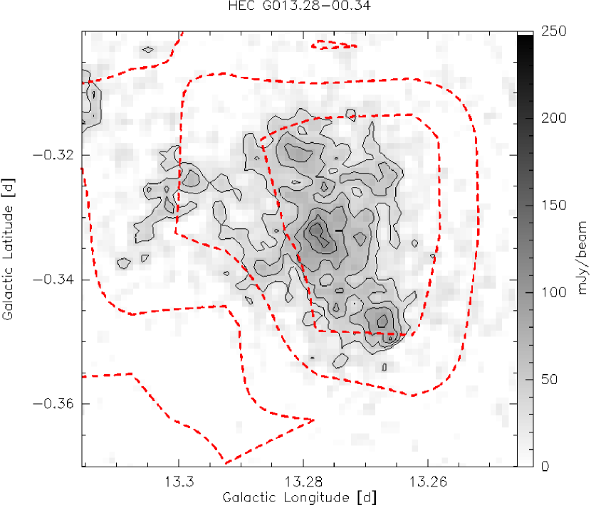
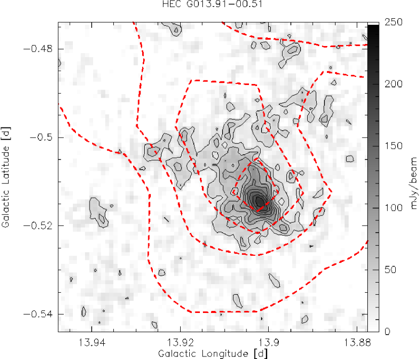
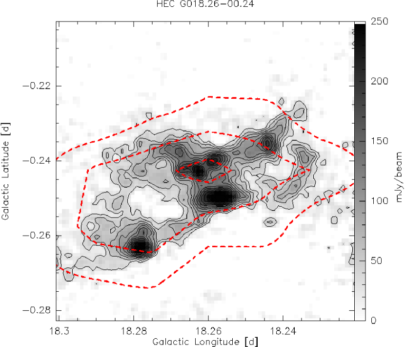
Figure 4: Examples of extinction maps (red dashed contour, starting at $A_{\mathrm{V}}$=21 mag and increasing by 10 magnitudes, beam 54″) on top of the 1.2 mm emission observed with MAMBO-2 (beam $10\hbox to0.0pt{$.$\hss}\,\arcsec 5$) in greyscale and solid black contours.

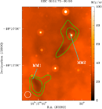
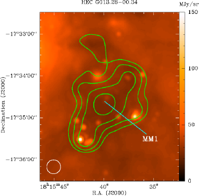
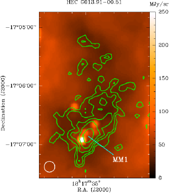
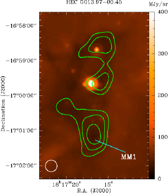
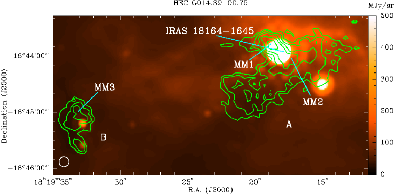
Figure 5: Spitzer/MIPS 24 $\mathrm{\mu m}$ images overlaid with the 1.2 mm continuum emission contours starting at $2\sqrt{2}\sigma$ ($\sigma=0.015$ Jy beam^-1) and increasing by factors of $\sqrt{2}$. The 1.2 mm clumps are labeled with their designation (as listed in Table 3, 7 and 5). In the bottom left corner we indicate the original MAMBO beam at 1.2 mm ($10\hbox to0.0pt{$.$\hss}\,\arcsec 5$), or the smoothed beam (20″) when a smoothed map is shown. Additionally, 6.7 GHz methanol masers (cyan triangles), water masers (blue squares), Hii regions (green pentagons with black contours), and IRAS sources are marked in the images. The 1.2 mm continuum emission maps are available in fits format on the CDS.

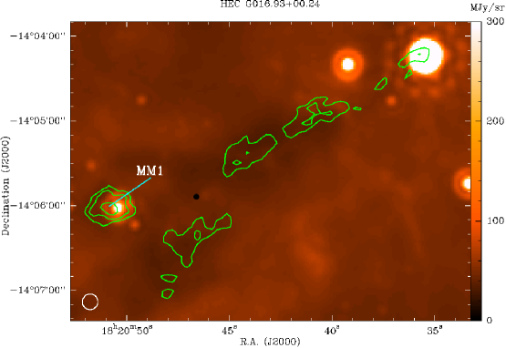
Figure 5: –Continued.

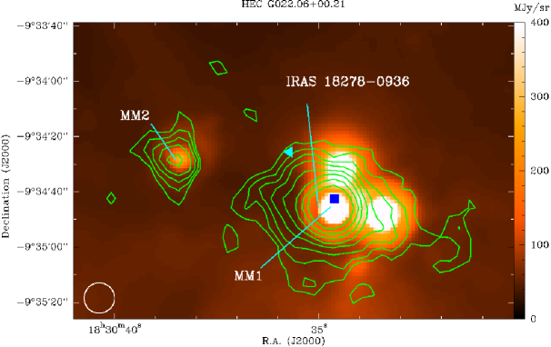
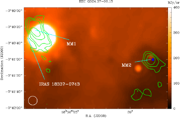
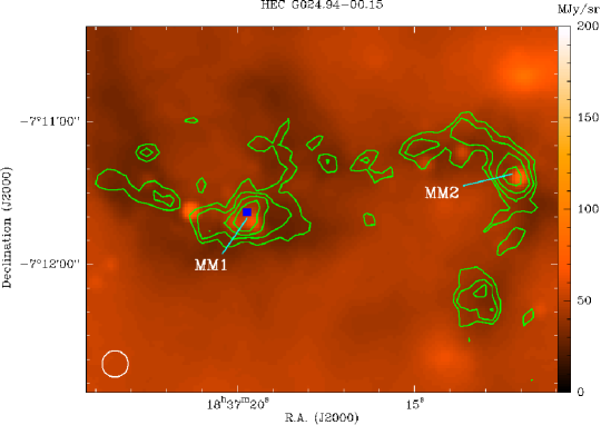
Figure 5: –Continued.

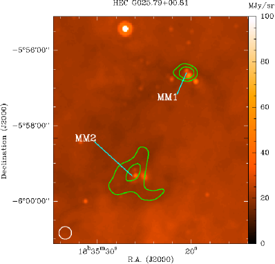
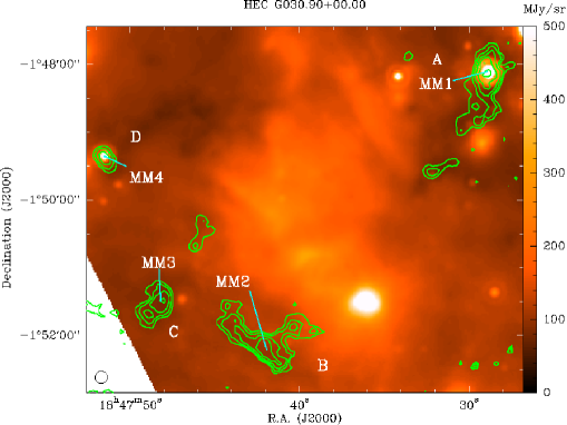
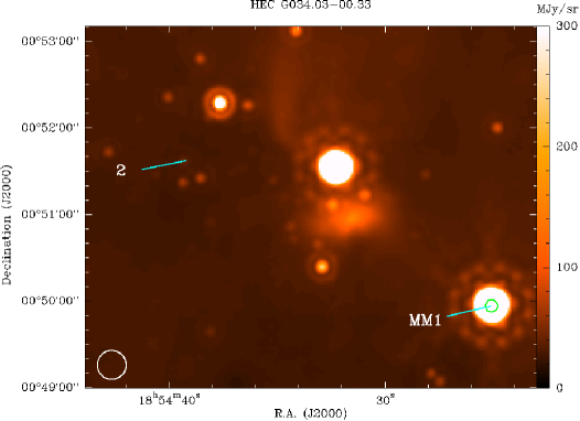
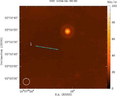
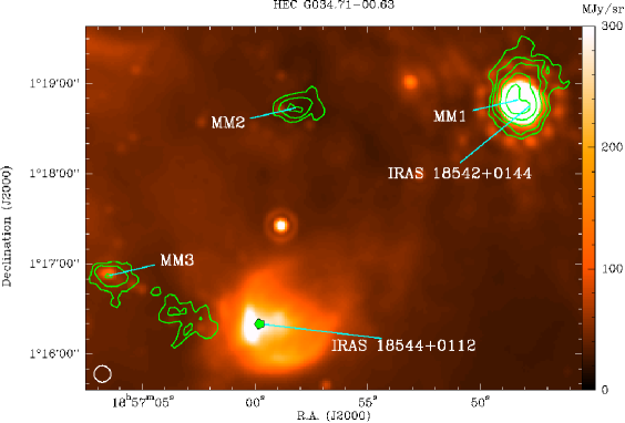
Figure 5: –Continued.

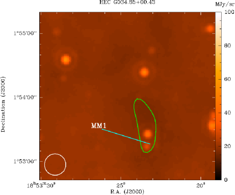
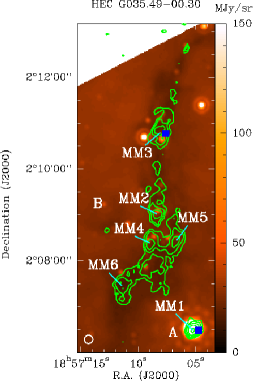
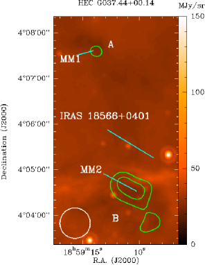
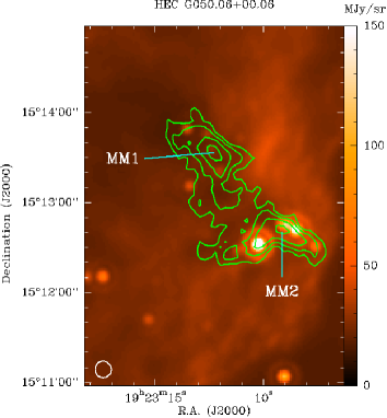
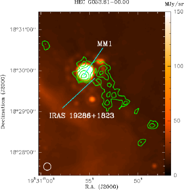
Figure 5: –Continued.

Millimeter continuum emission was detected in 88% of the bolometer maps. It usually followed well the 54″ resolution extinction maps (Fig. 4). Two examples of weak millimeter emission or non-detections are G034.03–00.33 and G034.34–00.90 (Fig. 5). Figure 5 shows the 24 $\mu$m maps from the Multiband Imaging Photometer for Spitzer (MIPS) overlaid with the mm emission. While the high extinction clouds match well with 24 $\mu$m dark features, the 1.2 mm peaks often contain weak compact 24 $\mu$m emission. The bolometer maps were sensitive to structures from $10\hbox to0.0pt{$.$\hss}\,\arcsec 5$ (FWHM) to $\sim$ 90$\arcsec$; large-scale structures are not faithfully represented due to the sky noise subtraction and chopping. We smoothed the maps, by convolving with a 20″ Gaussian beam, to study the extended cloud structure and increase the signal-to-noise toward weak and diffuse sources.

We find single clouds and clusters of clouds, for example G014.63–00.57 in Fig. 5. Based on the kinematic distance the clouds were identified as belonging together in one large cloud, or being physically separated clouds if the difference in distance was larger than 10%. The latter clouds were marked as A, B etc. and were treated as distinct clouds throughout the paper. For the total integrated flux of the cloud (Table 2), we defined a cloud edge at a threshold of $3\sigma$ (of the smoothed map) and integrated all the emission within this region using the Gildas Software package GREG. The corresponding radius of the cloud, $\sqrt{A/\pi}$ with $A$ the surface of the cloud, is given in arcseconds and parsecs (using the kinematic distance) in Table 2. The average cloud radius was 0.7 pc. Certain clouds have spherical shapes, for example G013.28-00.34, however, most are filamentary, as can be seen in G024.94-00.15 or G016.93+00.24. Cloud sizes are very diverse depending on the geometry; there are elongated structures up to several parsecs in length. The number of clumps per cloud varies from five (in G018.26-00.24, Fig. 5) to one or none in very diffuse clouds (G034.85+00.43, Fig. 5). We used the SIMBAD database to investigate if our clouds contain signs of star formation, such as maser emission, Hii regions, and IRAS sources.

4.4 Clumps in high extinction clouds

To study the clumps we used the unsmoothed maps, as the extended structure surrounding the clump complicates the definition of source edge and confuses Gaussian fitting routines. We removed the extended emission from the map by applying a median filter with a box size of 63″ (6 $\times$ beamsize) using the MIRIAD task ‘immedian’. After median removal, the source-find algorithm of MIRIAD, ‘sfind’, was run on these images delivering 2D Gaussian fits, the peak flux, and the integrated fluxes of the clumps. The median removal should strip the low density mass reservoir which surrounds the denser part of the clump.

Figure 6: Number distribution of 1.2 mm clumps with size determined from Gaussian fits and converted to physical units using the near kinematic distance.

Figure 7: Distance as a function of clump mass (left) and size (right). In the left panel, the clump mass based on Gaussian fitting is marked by squares, and the clump mass within 0.25 pc around the center of a clump is indicated by crosses. There is a linear correlation with distance for the mass and the size. The most massive clumps are at large distances, whereas almost no low-mass clumps are found at distances larger than 4 kpc, which can be expected for a sensitivity limited selection of clouds.

First, we selected the peaks in the mm emission by eye, and then we took the parameters for the FWHM size, the integrated flux and peak flux of the clump from ‘sfind’. The observed parameters of the clumps are presented in Table 3. The clumps have sizes (geometrical mean of the major and minor axis of the clump) of $10-30$″ or $0.11-0.72$ pc, peaking around 0.25 pc (Fig. 6). Most of the clumps are resolved with the $10\hbox to0.0pt{$.$\hss}\,\arcsec 5$ beam of the 30m telescope. The (physical) clump size follows a linear trend with distance (Fig. 7, right panel). At far distances we observe only larger, hence brighter clumps, which is expected for our sensitivity limited selection. The angular sizes, however, are more equally distributed (see Table 3). For several clouds with very weak mm emission the selected position was not the mm emission peak, but the emission center. In such clouds ‘sfind’ did not find any clumps; these positions without clumps are listed in Table 4.

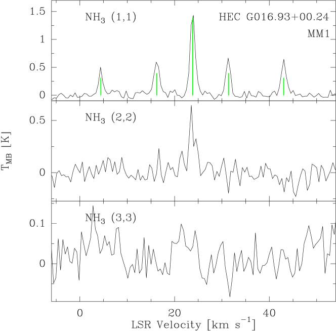
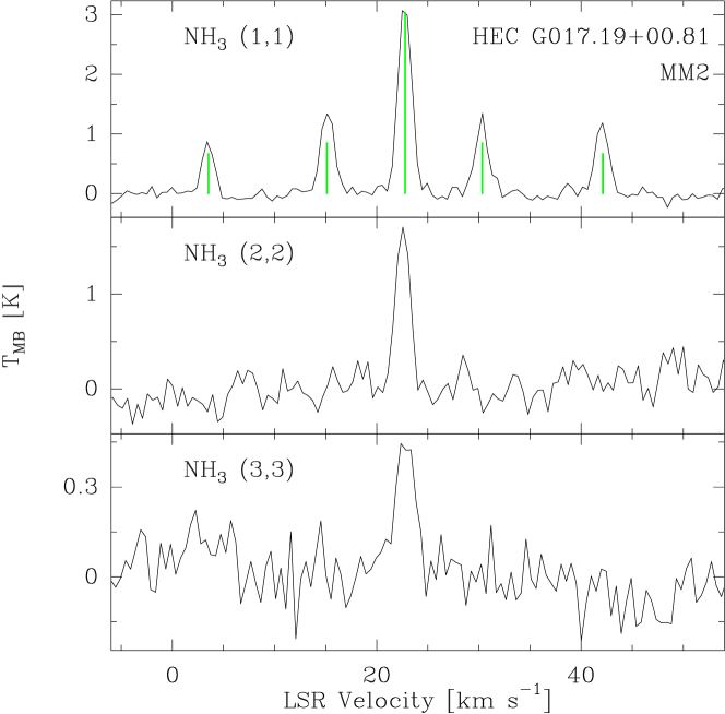
Figure 8: The $\mathrm{NH_{3}}$(1,1), $\mathrm{NH_{3}}$(2,2) and $\mathrm{NH_{3}}$(3,3) spectra taken with the Effelsberg 100m telescope toward two HEC clumps. The green lines indicate the theoretical intensity of the hyperfine lines given the intenstity of the main line.

Ammonia emission was detected toward 94% of the observed positions. Figure 8 shows the spectra of the $\mathrm{NH_{3}}$(1,1), $\mathrm{NH_{3}}$(2,2) and $\mathrm{NH_{3}}$(3,3) transitions toward two compact clumps representing typical values for an early stage where the clump is cold (14 K, G016.93+00.24 MM1) and a more evolved stage, where the temperature has increased (19 K, G017.19+00.81 MM2). In the early stage the $\mathrm{NH_{3}}$(3,3) line is not detected, while for the warmer clump it is clearly present. The results of the ammonia observations are summarized in Table 5. The main beam brightness temperatures of the $\mathrm{NH_{3}}$(1,1) lines are, after baseline removal, between 0.5 and 4.0 K. The baseline r.m.s. is $\sim$0.2 K, but several spectra are more noisy. The line widths from the main component of the $\mathrm{NH_{3}}$(1,1) range between 0.7 and 2.8 km s^-1, yielding an average of 1.4 km s^-1(Fig. 9). These line widths are far above a thermal linewidth, which would be around 0.23 km s^-1 for temperatures of $\sim$18 K. For most of the sources, the $\mathrm{NH_{3}}$(1,1) and $\mathrm{NH_{3}}$(2,2) lines are both detected, while the $\mathrm{NH_{3}}$(3,3) line is often very weak or not present. The $\mathrm{NH_{3}}$(2,2) and $\mathrm{NH_{3}}$(3,3) lines are on average both wider than the main $\mathrm{NH_{3}}$(1,1) line. This implies that these lines do not trace exactly the same volume of gas, meaning that the beam filling factor is not identical.

Figure 9: Number distribution of the $\mathrm{NH_{3}}$(1,1) line widths of the 1.2 mm clumps.

5 Analysis

Table 7: Properties of the clumps derived from $\mathrm{NH_{3}}$ and the 1.2 mm continuum.

HEC name		$d_{\mathrm{kin}}$	$A_{V}$	$FWHM$	${N_{\mathrm{H_{2}}}}$	${n_{\mathrm{H_{2}}}}$	$M_{\mathrm{1.2\,mm}}$	$M_{0.25pc}$	$M_{\mathrm{vir}}$	$T_{\mathrm{rot}}$	${N_{\mathrm{NH_{3}}}}$
		(kpc)	(mag)	(pc)	($10^{22}$ cm-2)	($10^{5}$ cm-3)	($\mathrm{M_{\odot}}$)	($\mathrm{M_{\odot}}$)	($\mathrm{M_{\odot}}$)	(K)	($10^{15}$ cm-2)
G012.73-00.58..	MM1	1.1	47	0.11	4.5	2.8	12	22	6	9.3(0.7)	3.7(0.8)
G013.28-00.34..	MM1	4.0	31	0.39	2.9	0.5	93	62	104	14.9(2.0)	3.2(1.1)
G013.91-00.51..	MM1	2.7	82	0.28	7.7	2.2	145	113	50	14.1(1.3)	2.5(0.5)
G014.39-00.75A..	MM1	2.2	61	0.21	5.7	2.0	52	47	31	17.4(2.0)	1.1(0.6)
G014.39-00.75B..	MM3	2.5	61	0.23	5.7	1.8	62	90	19	11.8(1.5)	2.4(0.8)
G014.63-00.57..	MM1	2.2	280	0.24	26.3	7.7	323	289	82	18.1(1.3)	4.7(0.5)
	MM2	2.2	164	0.15	15.4	7.3	72	80	26	15.7(1.1)	2.7(0.4)
	MM3	2.1	55	0.17	5.2	2.2	31	32	34	15.8(1.9)	3.4(0.8)
	MM4	2.3	32	0.18	3.0	1.2	21	26	12	19.1(5.9)	2.0(1.1)
G016.93+00.24..	MM1	2.4	44	0.27	4.2	1.1	64	53	23	14.0(1.3)	1.7(0.3)
G017.19+00.81..	MM1	2.5	52	0.23	4.9	1.5	54	58	35	17.2(0.9)	2.1(0.2)
	MM2	2.3	186	0.20	17.4	6.3	142	156	35	18.7(1.1)	2.1(0.2)
	MM3	2.3	56	0.25	5.3	1.5	72	108	45	20.0(1.5)	2.6(0.3)
	MM4	2.3	31	0.26	2.9	0.8	40	39	211	20.1(2.1)	3.2(1.1)
G018.26-00.24..	MM1	4.7	104	0.39	9.8	1.8	306	201	91	18.2(1.1)	4.3(0.4)
	MM2	4.7	95	0.48	8.9	1.3	431	208	201	17.4(1.2)	6.5(0.6)
	MM3	4.7	76	0.29	7.1	1.7	130	113	150	15.7(1.5)	6.4(0.9)
	MM4	4.7	61	0.30	5.7	1.3	110	88	140	16.6(1.1)	5.3(0.6)
	MM5	4.6	63	0.47	6.0	0.9	278	145	197	16.8(1.7)	6.0(1.0)
G022.06+00.21..	MM1	3.7	270	0.27	25.4	6.8	384	346	81	24.7(3.3)	4.9(0.9)
	MM2	3.7	84	0.24	7.9	2.4	92	74	36	15.5(1.6)	2.6(0.5)
G023.38-00.12..	MM1	5.6	70	0.50	6.5	0.9	346	163	134	18.1(1.2)	4.4(0.5)
G024.37-00.15..	MM1	3.9	52	0.38	4.9	1.1	165	110	174	18.6(1.9)	7.1(1.2)
	MM2	3.8	47	0.30	4.4	1.2	94	74	70	15.7(1.5)	3.8(0.7)
G024.61-00.3.3.	MM1	3.1	63	0.34	5.9	1.2	140	106	69	17.5(1.9)	2.0(0.4)
	MM2	3.2	38	0.31	3.5	0.8	72	49	21	15.5(1.2)	1.5(0.2)
G024.94-00.15..	MM1	3.3	69	0.26	6.5	2.0	104	94	61	15.2(1.0)	3.8(0.4)
	MM2	3.4	59	0.25	5.5	1.8	85	67	52	15.2(1.1)	3.5(0.5)
G030.90+00.00A..	MM1	4.6	55	0.53	5.2	0.7	311	131	125	18.6(1.7)	3.1(0.6)
G030.90+00.00B..	MM2	7.2	61	0.76	5.8	0.5	702	736	497	..	..
G030.90+00.00C..	MM3	5.7	46	0.56	4.3	0.5	283	126	71	16.4(2.4)	3.4(0.9)
G030.90+00.00D..	MM4	2.6	101	0.21	9.5	3.2	49	95	22	..	..
G034.71-00.63..	MM1	3.0	61	0.43	5.8	1.0	224	129	130	17.8(1.1)	2.2(0.3)
	MM2	3.0	55	0.33	5.2	1.1	122	83	59	12.4(0.9)	4.4(0.7)
	MM3	3.1	26	0.29	2.5	0.6	43	38	59	17.1(1.9)	1.0(0.4)
G035.49-00.30A..	MM1	3.6	71	0.26	6.6	1.8	98	89	100	18.6(2.9)	1.7(1.0)
G035.49-00.30B..	MM2	3.0	57	0.25	5.3	1.5	72	49	26	11.9(0.7)	3.9(0.5)
	MM3	3.0	44	0.38	4.2	0.8	127	81	102	13.6(0.7)	4.3(0.4)
	MM4	3.0	39	0.26	3.7	1.0	54	36	..	..	..
	MM5	3.0	40	0.28	3.8	1.0	64	46	..	..	..
	MM6	3.0	36	0.34	3.3	0.7	83	55	..	..	..
G050.06+00.06..	MM1	4.8	47	0.47	4.4	0.7	208	104	83	14.9(2.2)	2.1(0.6)
	MM2	4.8	49	0.49	4.6	0.7	233	106	87	14.1(1.7)	1.7(0.5)
G053.81-00.00..	MM1	1.9	74	0.14	6.9	3.6	28	36	28	12.4(1.4)	2.1(0.5)

Notes. The first two columns give the HEC name and the millimeter clump number, the following columns represent (in order of appearance): kinematic distance, visual extinction based on $N_{\mathrm{H_{2}}}$ from the 1.2 mm emission, size at FWHM, hydrogen column density, hydrogen volume density, mass, mass within 0.25 pc diameter, virial mass, $\mathrm{NH_{3}}$ rotational temperature, and $\mathrm{NH_{3}}$ column density.

5.1 Extinction masses

Since the color excess, or extinction, is a direct measure of the amount of column density in a region, we could derive extinction masses. One magnitude of $A_{V}$ is related to a hydrogen column density, $N_{\mathrm{H_{2}}}$, according to Bohlin et al. (1978) and Frerking et al. (1982) by

$$A_{V}=\frac{N_{\mathrm{H_{2}}}}{0.94\times 10^{21}}\hskip 14.22636pt[\mathrm{mag}].$$ (5)

Multiplying by the mass of a hydrogen atom, $m_{\mathrm{H}}$, the mean molecular weight, $\mu=2.33$, and the cloud surface, $A$, one arrives at the extinction mass:

$$M_{\mathrm{ext}}=3.7\times 10^{26}\mu m_{\mathrm{H}}<E(3.6\,\mu\mathrm{m}-4.5\,\mu\mathrm{m})>\big{(}\frac{A}{\mathrm{pc^{2}}}\big{)}\hskip 14.22636pt[\mathrm{M_{\odot}}].\\$$ (6)

The extinction mass is independent of temperature, but it still depends on the distance via the cloud surface $A$. We derive extinction masses for the clouds from $\sim$30 to 6500 $\mathrm{M_{\odot}}$ (Table 2).

5.2 Column densities and visual extinction

As mm emission from cool clouds is usually optically thin, the column density and the mass of a cloud are well sampled by the observed flux density. The beam averaged column density is given by Motte et al. (2007):

$$N_{\mathrm{H_{2}}}=\frac{F^{p}_{1.2\mathrm{mm}}}{\Omega m_{\mathrm{H}}\mu\kappa_{1.2\mathrm{mm}}B_{1.2\mathrm{mm}}(T_{\mathrm{dust}})}\,,$$ (7)

where $F^{p}_{1.2\mathrm{mm}}$ is the peak flux, $\Omega$ the beam solid angle, $\kappa_{1.2\mathrm{mm}}$ the dust opacity at 1.2 mm per unit mass column density, assuming a gas-to-dust ratio of 100, $B_{1.2\mathrm{mm}}(T_{\mathrm{dust}})$ the (full) Planck function at the dust temperature, and $m_{\mathrm{H}}$ and $\mu$ as defined before. The column density depends strongly on the dust properties: the dust opacity, $\kappa_{\lambda}$, and the emission coefficient, $\beta$, are related as $\kappa_{\lambda}=\kappa_{0}(\frac{\lambda}{\lambda_{0}})^{-\beta}$. We considered two different opacities; $\kappa_{\mathrm{1.2mm}}=0.4\,\mathrm{cm^{2}g^{-1}}$ after Hildebrand (1983) and $\kappa_{\mathrm{1.2mm}}=1.0\,\mathrm{cm^{2}g^{-1}}$ taken from Ossenkopf & Henning (1994), Table 1 column 6, for dust grains with thin ice mantles. The emission coefficient was kept at $\beta=2$, the advocated value for cold dust clumps (Hill et al., 2006). The dust opacities differ by a factor 2.5, meaning the $\kappa$ of Hildebrand (1983) results in 2.5 times larger column densities than the opacity of Ossenkopf & Henning (1994). In this work we used the dust opacity of Ossenkopf & Henning (1994), $\kappa_{\mathrm{1.2mm}}=1.0\,\mathrm{cm^{2}g^{-1}}$. For the dust temperature we assumed the rotational temperature derived from ammonia (see Section 5.5). Since the clumps have high densities, collisions will dominate over radiative processes and the temperature exchange between dust and gas will be efficient. In sources without $\mathrm{NH_{3}}$ detection we assumed a dust temperature of 16 K, which was the average $\mathrm{NH_{3}}$ rotational temperature. For clumps which have an embedded protostar the $\mathrm{NH_{3}}$ rotational temperature, derived on a 40″ scale, might underestimate the dust temperature leading to an overestimation of the derived masses and column densities.

We found clumps with column densities of the order of $10^{22}-10^{23}\,\mathrm{cm^{-2}}$ (Table 7). We derived corresponding peak visual extinction values by applying Eq. 5. The peak fluxes, column densities and peak visual extinction of Table 7 correspond to the positions listed in Table 3. The clumps have peaks in $A_{\mathrm{V}}$ from 31 to 280 mag, with an average value of 75 mag. These values are much higher than the mean visual extinction reached by the extinction method for this selected sample, which is between 16 and 47 mag. This is expected because the peak values are larger than the mean and with the limited resolution of 54″ higher extinction peaks (as found for example in IRDCs) are missed. Additionally, also the temperature might play a role, since the derivation of the $A_{\mathrm{V}}$ from the mm emission depends on temperature while the extinction method does not.

5.3 Masses from 1.2 mm emission

The clump mass can be derived from the 1.2 mm emission by (Hildebrand, 1983; Motte et al., 2007):

$$M_{\mathrm{1.2mm}}=\frac{F^{i}_{\mathrm{1.2mm}}d^{2}}{\kappa_{\mathrm{1.2mm}}B_{\mathrm{1.2mm}}(T_{\mathrm{dust}})}\,,$$ (8)

where $F^{i}_{\mathrm{1.2mm}}$ is the integrated flux density of the clump, $d$ the distance, and $\kappa_{\mathrm{1.2mm}}$, $B_{\mathrm{1.2mm}}$, and $T_{\mathrm{dust}}$ as defined before. The measured flux density can be contaminated by free-free emission if an ionizing source is present. Since our sample contained very young objects, we can neglect such contamination. The derived masses depend strongly on temperature and distance; a $10\%$ nearer distance decreases the mass by $20\%$, a $10\%$ decrease in temperature increases the mass by $17\%$. Nevertheless, the largest uncertainty in the mass derivation is caused by the dust properties, as described in the previous section.

The majority of the clumps have masses between 12 and 700 $\mathrm{M_{\odot}}$ and are located at distances between 2 and 5 kpc (see the squares in the left panel of Fig. 7 and Table 7). We find no low-mass clumps ($M<100\,\mathrm{M_{\odot}}$) further than 4 kpc, which is an bias of our extinction method (discussed in Sect. 6.4). Almost all high mass clumps ($M>100\,\mathrm{M_{\odot}}$) are located at distances larger than 4 kpc.

A second method was used as a comparison for the clump masses to check if the source finding algorithm was biased to a source size (and hence clump mass). Based on the (near) kinematical distances, we defined circles of 0.25 pc diameter for each source. Then, we derived the integrated flux, $F_{0.25\mathrm{pc}}$, and the mass, $M_{0.25\mathrm{pc}}$, for the region within this circle (see Tables 3, 7 and 4). The crosses in the left panel of Fig. 7 show $M_{0.25\mathrm{pc}}$ as a function of the distance. The clump masses within 0.25 pc show a similar behavior as the clump masses determined by Gaussian fits. On a larger scale, the cloud mass was derived from the 1.2 mm emission according to Eq. 8 using the integrated flux down to 3$\sigma$. The cloud diameters are of order $\sim$90″, so after resampling the extinction map, it was possible to compare the cloud masses derived by extinction with the masses from the 1.2 mm emission. We find the extinction masses to be larger by a factor $\sim 1.3$ than the masses derived from the dust continuum maps (see Fig. 10). This is expected, since the bolometer filters out large-scale structures by the sky noise subtraction and chopping. The cloud masses derived from the 1.2 mm emission and the extinction are listed in Table 2.

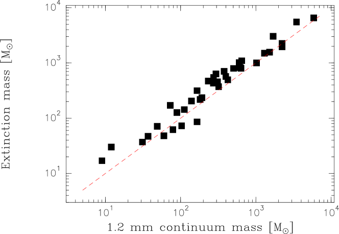
Figure 10: The cloud masses estimated from the color excess versus the masses estimated from the 1.2 mm continuum maps. The red dashed line is a help line indicating the trend in which both mass estimates are equal.

Finally, we estimated the volume-averaged gas density of the clumps, $n_{\mathrm{H_{2}}}$, following Motte et al. (2007):

$$n_{\mathrm{H_{2}}}=\frac{M}{\frac{4}{3}\pi R^{3}\mu m_{\mathrm{H}}}\,,$$ (9)

where $M$ is the clump mass, $R$ the clump radius given by the geometrical mean of the semi major and semi minor axis from the Gaussian fit. The average gas density is $\sim 2\times 10^{5}\,\mathrm{cm^{-3}}$ and the individual results are given in Table 7.

5.4 Virial masses

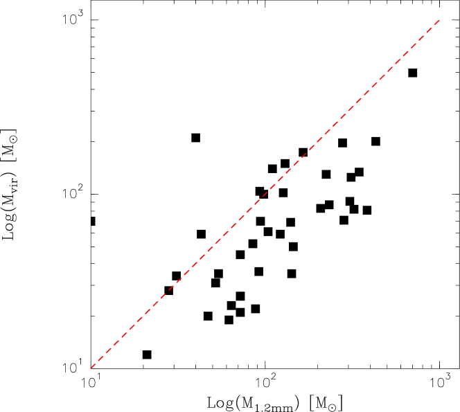
Figure 11: Virial clump masses versus the 1.2 mm continuum clump masses. The red dashed line indicates the trend where the virial parameter is unity.

The thermal line widths are usually one order of magnitude smaller than the observed $\mathrm{NH_{3}}$ line widths, which indicates that the observed line widths are dominated by turbulence, hence contain information of the average kinetic energy within a clump.

Given an optically thin line width and a clump radius, the virial mass, $M_{\mathrm{vir}}=k_{1}\sigma^{2}R/G$, can be calculated (MacLaren et al., 1988). Here $\sigma$ is the three dimensional root-mean-square velocity, $R$ the clump radius and $k_{1}$ a density distribution constant. For a constant density distribution $k_{1}=5/3$. After the conversion of $\sigma$ to the observable FWHM line width $\Delta v$, $\sigma^{2}=(3/8\ln 2)\Delta v^{2}$ (Rohlfs & Wilson, 2004), the virial mass can be written as:

$$M_{\mathrm{vir}}=210\times\big{(}\frac{\Delta v}{\mathrm{km\,s^{-1}}}\big{)}^{2}\big{(}\frac{R}{\mathrm{pc}}\big{)}\hskip 14.22636pt[M_{\odot}].$$ (10)

The resultant virial masses, $M_{\mathrm{vir}}$, are listed for each clump in Table 7. The virial parameter is defined as $\alpha=\frac{M_{\mathrm{vir}}}{M}$ (Bertoldi & McKee, 1992). For $\alpha<1$ , the clumps are dominated by gravity, however with $\alpha>>1$, the clumps are confined by surface pressure and self-gravity is unimportant. Most clumps in high extinction clouds have clump masses larger than their virial masses (see Fig. 11), indicating that possibly most clumps are dominated by gravity and are collapsing.

5.5 Temperatures

The ammonia molecule, described thoroughly by Ho & Townes (1983), is often used as a molecular cloud thermometer (Danby et al., 1988). Its energy levels are parameterized by the $J$ and $K$ quantum numbers, measuring, respectively, the magnitude of the total angular momentum and its component along the symmetry axis. Each set of rotational transitions is arranged into so-called $K$-ladders, levels of fixed $K$-value. From the symmetry of the electric dipole moment of the molecule, all dipole transitions with nonzero $\Delta K$ are forbidden, meaning that the $K$-ladders are independent of each other. The lowest transitions of each $K$-ladder are metastable, and can be excited via collisions. Additionally, $\mathrm{NH_{3}}$ also undergoes vibrational motion from the tunneling of the nitrogen atom through the hydrogen plane, which splits the rotational energy levels into inversion doublets.

The inversion transitions are further split into five quadrupole hyperfine lines, which allow the calculation of the optical depth (see the hyperfine lines in the $\mathrm{NH_{3}}$(1,1) transition in Fig. 8). Typical values of the optical depth were between 1 and 3, showing that ammonia is optically thick in most cases. With the optical depth known, the rotational temperature follows from the ratio of the peak intensities of $\mathrm{NH_{3}}$(1,1) and $\mathrm{NH_{3}}$(2,2) lines after Mangum et al. (1992):

$$T_{\mathrm{rot}}=-41.5\big{[}\ln\big{[}-\frac{0.283\Delta v_{22}}{\tau_{\mathrm{main}}\Delta v_{11}}\ln\big{[}1-\frac{T_{22}}{T_{11}}(1-e^{-\tau})\big{]}\big{]}\big{]}^{-1}\hskip 14.22636pt[\mathrm{K}],$$ (11)

where $\tau_{\mathrm{main}}$ is the $\mathrm{NH_{3}}$(1,1) main group optical depth, $\Delta v_{11}$, $\Delta v_{22}$, $T_{11}$, $T_{22}$ are the line widths and the peak intensities of the $\mathrm{NH_{3}}$(1,1) and $\mathrm{NH_{3}}$(2,2) lines, respectively.

The line width ratio in this equation is debatable. Observations show that the $\mathrm{NH_{3}}$(1,1) and $\mathrm{NH_{3}}$(2,2) line widths are dominated by turbulence. If one assumes that both transitions arise from the same region, they experience the same turbulence, and the line widths are equal, $\Delta v_{22}=\Delta v_{11}$. In this case, the linewidth ratio drops out of the equation, which becomes the equation from Ho & Townes (1983). We observed slightly larger $\mathrm{NH_{3}}$(2,2) line widths for several clumps, probably since this transition has a higher energy and is therefore more sensitive to warmer and more turbulent regions. The $\mathrm{NH_{3}}$(2,2) line widths are therefore more sensitive to the peak temperature, determined by the turbulent outliers. We considered it reasonable to use $\Delta v_{22}$ =$\Delta v_{11}$, since it would give an ‘average’ of the $\mathrm{NH_{3}}$(2,2) turbulence, and hence an ‘average’ rotational temperature of that region. The two methods yield very similar results; the Ho & Townes (1983) temperatures were slightly lower ($\Delta T_{\mathrm{rot}}\simeq 1$K) than when using the formula of Mangum et al. (1992).

The clumps are on average cold $\sim$16 K. The temperatures range from 10 to 25 K. For such low temperatures, the kinetic temperature is well approximated by $T_{\mathrm{rot}}$ (Walmsley & Ungerechts, 1983; Danby et al., 1988).

We derived column densities of the $\mathrm{NH_{3}}$(1,1) line (after Mangum et al., 1992):

$$N_{(1,1)}=6.60\times 10^{14}\Delta v_{11}\tau\frac{T_{\mathrm{rot}}}{\nu_{11}}\hskip 14.22636pt[\mathrm{cm}^{-2.}]$$ (12)

From this we estimated the total ammonia column density (following Li et al., 2003):

$$N_{\mathrm{NH_{3}}}=N_{(1,1)}\Big{[}1+\frac{1}{3}\exp\big{(}\frac{23.1}{T_{\mathrm{rot}}}\big{)}+\frac{5}{3}\exp\big{(}\frac{-41.2}{T_{\mathrm{rot}}}\big{)}$$

$$+\frac{14}{3}\exp\big{(}\frac{-99.4}{T_{\mathrm{rot}}}\big{)}\Big{]}\hskip 14.22636pt[\mathrm{cm}^{-2}].$$ (13)

The averaged ammonia column density for the clumps is $3.1\times 10^{15}\,\mathrm{cm^{-2}}$. The $\mathrm{NH_{3}}$ rotational temperatures and column densities for all clumps are given in Table 7 together with the other parameters derived in this Section.

6 Discussion

6.1 High extinction structures

Thanks to the high resolution Spitzer IRAC data, the extinction method allows to follow the mass distribution from Galactic size-scales down to single clouds. High extinction traces Galactic structure (see the Galactic distribution of the color excess in Fig. 2), similar to the CO survey of the Galactic plane (Dame et al., 1987) and the dust continuum surveys, ATLASGAL at 850 $\mathrm{\mu m}$ (Schuller et al., 2009) and BOLOCAM at 1.1 mm (Rosolowsky et al., 2009). In addition, the distribution of 6.7 GHz Class II methanol masers traces high-mass star-forming regions and, thus, Galactic structure (Pestalozzi et al., 2005). All these surveys, except for the methanol masers, peak toward the Galactic Center. The extinction maps miss the inner 1° around the Galactic Center, since the Spitzer IRAC data were not publicly available for this region at the time. However, a rising trend toward the Galactic Center was observed. The extinction distribution indicates that the column densities are higher towards the fourth quadrant, $0\degr>l>-60\degr$. We find no evidence for this from the CO distribution, nor from the methanol masers. Only the ATLASGAL survey (Schuller et al., 2009) hints at a similar distribution, but needs to be extended in longitude range for giving conclusive evidence.

The next eye-catching features in the extinction distribution were two bumps, peaking roughly around longitudes of $\sim 40\degr$ and $-30\degr$ (see Fig. 2), which were confirmed by the methanol maser distribution (Pestalozzi et al., 2005). We identified several spiral arms by comparing our results to the Galactic models of Vallée (2008). In Fig. 2 each spiral arm traced by a maximum in the extinction distribution is marked. We can trace the tangential point of the Sagittarius-Carina arm at $l\sim 50\degr$, the tangential points of the Scutum-Crux arm at $l\sim 35\degr$ and $l\sim-45\degr$, the beginning of the Norma-Cygnus arm on the near end of the Galactic bar $l\sim 10\degr$, the beginning of the Sagittarius-Carina arm at the far end of the Galactic bar $l\sim-5\degr$, the beginning of the Perseus arm $l\sim-20\degr$, and the tangential point of the Norma-Cygnus arm at $l\sim-30\degr$. Several of these features are also seen in the ATLASGAL survey, and to a lesser extent in the CO distribution. Hence, the total extinction distribution seems to agree with results of previous studies, and tracks large scale mass structures.

The combination of submillimeter dust continuum emission and extinction maps extends the size scales down to clump sizes of fractions of parsecs. In Table 8 the mean masses, radii, and volume densities for different size-scales of complexes, clouds and clumps are compared. Complexes are the low density ($A_{\mathrm{V}}>21\,\mathrm{mag}$ or $N_{\mathrm{H_{2}}}>2\times 10^{22}\,\mathrm{cm^{-2}}$) regions surrounding the cloud. In general, the masses and sizes decrease towards the smaller scales, while the volume density increases as expected. The cloud masses derived from the extinction are higher than from the mm emission, as discussed in Sect. 5.3. The complexes and the clouds are confined by the pressure of the surroudning medium rather than by gravity. This is based on their virial masses, where we used for the line width estimate the ¹³CO data from the Galactic Ring Survey (GRS) (Jackson et al., 2006). The ¹³CO line is a probe of the low density material and with the GRS resolution of 47″ the line width is represenative for a cloud-scale average. Most of the clumps inside the clouds are, however, bound objects for which $M_{\mathrm{vir}}<M_{\mathrm{1.2\,mm}}$.

Table 8: Mean properties of high extinction complexes, clouds and clumps

Size scale	Method	Mass	Radius	Vol. den.
		($\mathrm{M_{\odot}})$	(pc)	(cm-3)
complex	extinction	4000	1.4	6$\times 10^{3}$
clouds	extinction	910	0.7	1$\times 10^{4}$
clouds	1.2 mm emission	700	0.7	9$\times 10^{3}$
clumps	1.2 mm emission	130	0.15	2$\times 10^{5}$

6.2 Evolutionary sequence

Our observations suggest different classes of clouds and in the following we discuss their possible relation to different evolutionary stages. Clouds, which either have no clumps or clumps of which the peak in the mm emission is less than twice the mean emission in the cloud, were defined as diffuse clouds – this definition is based on the cloud morphology and therefore different from the “classical diffuse clouds” defined by $A_{\mathrm{V}}<1\,$mag (Snow & McCall, 2006). Clouds which contain clumps with a higher contrast, above twice the mean cloud emission, were considered to be peaked clouds. If the peak flux was above thrice the mean emission and there were two or more clumps the cloud was classified as a multiply peaked cloud. The ratio of the clump peak emission to the mean emission of the cloud is given in Table 2 together with the classification. The mean physical properties such as temperature, masses, column densities and line widths are put together in Table 9 for the three classes.

Diffuse clouds are the most likely candidates to form, or harbor, starless clumps, which are expected to be cold, more extended and more massive. The clump, or cloud, consists of low column density material and contains no massive compact object. Indeed, for very diffuse clouds, the source find algorithm yielded few clumps. On the smoothed maps, the algorithm returned values which were close to cloud size-scales without much substructure. This supports the idea that these diffuse clouds represent the earliest stage in which few condensations have formed and gravitational collapse has not yet started. More evidence for the young nature of diffuse clouds was found in the 24 $\mathrm{\mu}$m MIPS data: generally the (smoothed) dust emission followed the 24 $\mathrm{\mu}$m-dark regions and only a few 24 $\mathrm{\mu}$m sources of $\sim$100$\,\mathrm{MJy\leavevmode\nobreak\ sr^{-1}}$, located within 20″ of mm peak, were found toward the clouds. In two cases 24 $\mu$m source $>100\,\mathrm{MJy\leavevmode\nobreak\ sr^{-1}}$ were found the edge of the cloud, at $\sim$1′ from the mm peak. Examples are G012.73–00.58, G013.28–00.34, and G034.85+00.43 (see Fig. 5).

As the first clumps become more compact and their mm peak flux rises above twice the mean emission of cloud, in the peaked cloud stage, the clump is accreting material from a lower density reservoir or envelope surrounding it, and consequently the temperature and turbulence rise. Since star formation is a process which is dynamic and includes feedback and triggering, already in this early stage a cloud can contain more than one clump, though possibly the other peaks barely stick out above the mean mm emission of the cloud. The peaked clouds are generally dark at 24 $\mathrm{\mu}$m, except for a bright 24 $\mathrm{\mu}$m source located within 20″ of the mm peak (see G013.91–00.51, G016.93+00.24, and G053.81–00.00 in Fig. 5). The peak flux of the 24 $\mu$m sources is on average $\sim 250\,\mathrm{Mjy\leavevmode\nobreak\ sr^{-1}}$, which is higher than what was found for the diffuse clouds.

After more accretion from the reservoir, the clump will have a much higher mm peak flux compared to the initial stage, reaching at least trice the mean emission of the cloud. The clump mass will have decreased toward the more evolved stage, since not all of the mass reservoir will not be accreted onto the clump, as the star formation efficiency is apparently less then 100%. The column density, temperature and turbulence will increase even further than in the peaked cloud stage. While in the peaked stage, there were few clouds which had multiple clumps, in the more evolved stage one expects to find more clouds with multiple clumps. Most of these clumps should be well above the mean emission of the cloud. In these multiply peaked clouds, the clumps will be in different cloud stages of evolution depending on the initial conditions of the clump. Also not all clumps will form high-mass stars, so they will have different properties. And indeed, several clumps in the multiply peaked clouds show bright, $\gtrsim 500\,\mathrm{Mjy\leavevmode\nobreak\ sr^{-1}}$, 24 $\mathrm{\mu}$m emission, indicating a protostar, within 10″ or less of the mm peak, while other clumps are infrared dark. Such clouds with clumps in various phases are not completely infrared dark, since the dust is locally heated from the already hot HMPO or UCHii region. Examples for multiply peaked clumps are shown in Fig. 5: G014.63–00.57, with the very bright component MM1 and the cloud G018.26–00.24 with five clumps.

Additionally, one can check the evolutionary stage by searching for signs of star formation such as water masers, Class II methanol masers, and shocks. Table 9 also contains entries for such star formation tracers. Water masers are thought to be caused by outflows during (low and high-mass) star formation (Menten, 1996). The Class II methanol masers are uniquely associated with high-mass star formation, and are usually found prior or coexistent with an H ii region (Menten, 1991; Ellingsen, 2006; Pestalozzi et al., 2007). While the water masers are found towards both the peaked and the multiply peaked clouds, the methanol masers are only found toward the latter class. Another indication for star formation comes from gas excited by shocks, such as H₂($v$=0–0), $S$(9,10,11) or CO($v$=1–0) gas. The IRAC 4.5 $\mu$m band contains both these transitions, and can therefore be used to search for ongoing star formation. The close association of the extended 4.5 $\mu$m objects with Class II methanol masers, found by Cyganowski et al. (2008), suggests that they might trace ongoing massive star formation. We find two multiple peaked clouds in our sample that contain such an extended 4.5 $\mu$m source, of which one also contains Class II methanol masers.

The peaked and multiply peaked clouds show active star formation, while the diffuse clouds do not. Possibly, these clouds might not form stars or will not have column densities high enough to form massive stars. However, some, for example G013.28–00.34, seem to be forming clumps which might evolve into active star-forming clumps. Table 9 shows that the clump temperatures are very similar, especially in the case of peaked and the multiply peaked clouds; the diffuse clouds stand out with their temperature of $13.5\pm 1.5$ K against the average temperature of all clouds $16\pm 1.8$ K. As star formation produces stars in a large range of masses, so cluster-forming regions or clumps within one cloud are expected to have different column densities and temperatures. Given the range of column densities for the clumps $3-30\times 10^{22}\,\mathrm{cm^{-2}}$ not all clumps might evolve into clusters with massive stars, even if mass accretion is still continued from the low density material surrounding the clump.

Table 9: Mean physical properties of the clumps and star formation indicators in diffuse, peaked and multiply peaked clouds.

	Diffuse	Peaked	Multiply peaked
Mass ($\mathrm{M_{\odot}}$)	230	185	150
Size (pc)	0.52a	0.36	0.30
$N_{\mathrm{N_{H_{2}}}}$ ($10^{22}$cm-2)	4.5a	5.5	8.5
$T_{\mathrm{rot}}$ (K)	13.5	15.7	17.5
$\Delta v$ (km s-1)	1.2	1.4	1.6
IRDC corr. (within 2′)	83%	50%	70%
24$\mu$m (within 1′)	17%	83%	100%
Ext. 4.5$\mu$m (within 1′)	none	none	29%
Masers (within 1′)	none	$\mathrm{H_{2}O}$ 25%	$\mathrm{H_{2}O}$ 57%
			$\mathrm{CH_{3}OH}$ 29%

6.3 Comments on individual sources

We performed a systematic search using the SIMBAD Astronomical Database of our cloud to find signs of star formation such as maser emission, Hii regions and IRAS sources. We discuss here several diffuse, peaked and multiply peaked high extinction clouds, which are representative examples of typical clouds in our sample. Additionally, several unique and interesting clouds are mentioned.

6.3.1 G013.28–00.34

The cloud G013.28–00.34, with its one centrally located clump MM1, is a good example of a cloud in a very early phase of protocluster formation. This clump has a low column density $3\times 10^{22}\,\mathrm{cm^{-2}}$ and contains less than 5% of the total cloud mass. Likely, this clump did not yet start to collapse, since from the virial mass we know that the clump is confined by gas pressure. Additionally, the clump contains no 24 $\mu$m emission, which is a further evidence for stage prior to star formation. The moderate $\mathrm{NH_{3}}$ line widths of $1.6\,\mathrm{km\leavevmode\nobreak\ s^{-1}}$ indicate a source of turbulence or large scale motions, however, without an $\mathrm{NH_{3}}$ map of the cloud it is impossible to isolate the source for the turbulence.

6.3.2 G013.91–00.51

In the cloud G013.91–00.51 the 1.2 mm emission follows an infrared dark patch. The one clump in this cloud which is three times above the mean emission is located nearby two infrared emission peaks and can be possibly triggered by the star formation in these infrared bright sites. The clump is very massive, 145 $\mathrm{M_{\odot}}$, and cold. The virial mass is 50 $\mathrm{M_{\odot}}$ suggesting a collapse.

6.3.3 G014.63–00.57

Cloud G014.63–00.57 is nested around two bright infrared sources. The 1.2 mm peak fluxes are high, especially for clumps nearby the infrared sources. The brightest clump, MM1, contains a compact bright infrared source, IRAS 18164–1631, with a flux density at 25 $\mu$m $F_{\mathrm{25\mu m}}=23$ Jy (Helou & Walker, 1988) and has wide $\mathrm{NH_{3}}$ line widths of $1.8\,\mathrm{km\,s^{-1}}$ indicating large turbulence. Additionally, water masers were detected towards this clump (Jaffe et al., 1981) and Cyganowski et al. (2008) showed that there is extended 4.5 $\mu$m emission – a further indication for outflows. All evidence points to a state of ongoing star formation for the MM1 clump. The other clumps of G014.63–00.57 are still infrared dark. The MM1 and MM2 clumps have the theoretically required column density for massive star formation (see Sect. 6.6).

6.3.4 G016.93+00.24

In G016.93+00.24 the 1.2 mm emission follows the infrared dark filament. In the west end of the filament, the 1.2 mm peak MM1, is a few arc seconds offset from a infrared bright emission peak. The $\mathrm{NH_{3}}$ line widths are relatively narrow, $0.9\,\mathrm{km\leavevmode\nobreak\ s^{-1}}$, and the temperature is low, $14\,$K, which suggests that the clump is in a very early phase with little turbulence.

6.3.5 G017.19+00.81

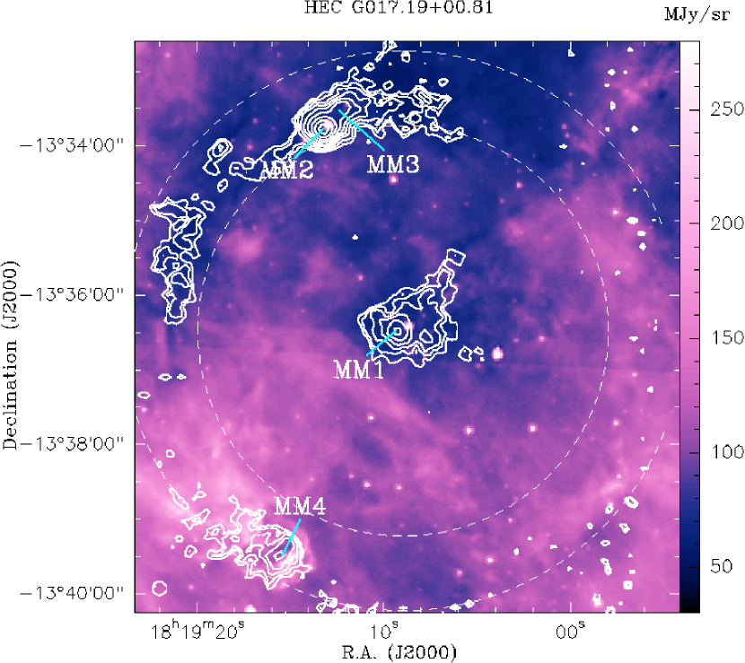
Figure 12: A Spitzer GLIMPSE 8.0 $\mu$m image of cloud G017.19+00.81 overlaid with the 1.2 mm emission in white contours starting at $2\sigma$ ($\sigma=0.015$ Jy beam^-1) and increasing by $\sqrt{2}$. All clumps are at the same kinematic distance of $2.3\pm 0.2$ kpc. The dashed circles guide the eye to the arc-like structure, which is infrared dark in the north-east and infrared bright in the south west.

The multiple peaked cloud G017.19+00.81 harbors several clumps, which are all at a kinematic distance of $2.3\pm 0.2$ kpc, arranged in an infrared dark arc (Figs. 5 and 12). Such a morphology might point to triggered star formation. The location of this cloud, on the edge of the bright Hii region M16, the Eagle nebula, suggests that we are observing new massive star-forming clumps in an early stage of evolution, whose creation might be linked to the already ongoing star formation in this region. G017.19+00.81 differs from the classical triggered star formation scenario described by Zavagno et al. (2005). First, the absence of an Hii region in the center of the arc; no radio emission was detected either in the 20 cm MAGPIS survey (Helfand et al., 2006), the 21 cm VLA survey (Condon et al., 1998), or in the 6 cm Parkes survey (Haynes et al., 1979) – the object was not covered by the 5 cm VLA survey (Becker et al., 1994). Second, an arc triggered by an Hii region is expected to be infrared bright, whereas G017.19+00.81’s arc is partially infrared dark.

The clumps in the cloud have similar temperatures and sizes. The upper two left clumps, MM2 and MM3, represent most of the mass in this cloud, whereas the southern MM4, shows the largest amount of turbulence. Toward the MM2 clump we detected water masers, within a beam of 40″. It is coincident with a bright 24 $\mu$m source indicating a protostar. MM2 seems to be an evolved clump, where star formation is just beginning. Additionally, the column density of this clump theoretically allows high-mass star formation. The MM4 clump is located nearby an Hii region, which might explain the wide line width of $2.8\,\mathrm{km\leavevmode\nobreak\ s^{-1}}$ and high degree of turbulence. Nearby (1′) there is an infrared-bright source, IRAS 18164–1340, which is only detected at long mid-infrared wavelengths of 100 $\mu$m ($F_{\mathrm{100\mu m}}=770$ Jy, Helou & Walker, 1988) We performed a more detailed study of this region; a molecular line survey with IRAM 30m and an interferometer study with the SMA (Rygl et al. , in preparation).

6.3.6 G018.26–00.24

G018.26–00.24 is a cloud with five 1.2 mm peaks located northward of an infrared bright region with several Hii regions and water maser detections. There are several infrared sources present in the cloud, however, the most mm emission peaks are infrared dark. MM3 is an exception, here the infrared peak is just a few arc seconds from the mm peak. MM1 has the largest separation from the infrared bright region. This clump has the highest column density and the narrowest line width of the five clumps in this cloud. The overall cloud shape suggests that the gas and dust was collected by a driving force south-west of the cloud, possibly the infrared bright source at ($\alpha=18^{\mathrm{h}}25^{\mathrm{m}}02\hbox to0.0pt{$.$\hss}\,^{\mathrm{s}}8,\delta=-13\degr 09\arcmin 30\arcsec$, J2000).

6.3.7 G022.06+00.21

G022.06+00.21 contains one clump with a bright mm peak, MM1, and second clump with a weaker peak, MM2. MM1 is coincident with IRAS 18278–0936 ($F_{\mathrm{25\mu m}}=12$ Jy, Helou & Walker, 1988), has 6.7 GHz methanol masers (Szymczak et al., 2000), extended 4.5 $\mu$m emission (Cyganowski et al., 2008), and has a sufficient column density for high-mass star formation. Additionally, we detected water masers towards MM1, within a beam of 40″. MM1 is a relatively warm clump, $25\,\mathrm{K}$, with ongoing star formation suggested by the masers and outflow tracers. MM2 is more quiescent and coincident with a weak infrared source.

6.3.8 G024.37–00.15

G024.37–00.15 contains two clumps, one infrared bright, MM1, and one infrared dark, MM2. MM1 coincides with the bright IRAS source 18337–0743 ($F_{\mathrm{25\mu m}}=47$ Jy, Helou & Walker, 1988), and has a wide linewidth $2.1\leavevmode\nobreak\ \mathrm{km\leavevmode\nobreak\ s^{-1}}$. The MM2 core is in an earlier state of star formation, exhibiting SiO emission (Beuther & Sridharan, 2007) and water masers.

6.3.9 G024.61–00.33

In G024.61–00.33, the strongest mm emission peak, MM1, is coincident with IRAS 18346–0734 ($F_{\mathrm{25\mu m}}=25$ Jy, Helou & Walker, 1988) and nearby, separated by $\sim 30\arcsec$, Szymczak et al. (2000) detected 6.7 GHz methanol masers. The second clump, MM2, is infrared dark.

6.3.10 G024.94–00.15

The mm emission follows closely the infrared dark filament in cloud G024.94–00.15. The clumps, MM1 and MM2, are located near weak infrared sources. We found water maser emission toward MM1, within a beam of 40″, indicating early phases of star formation.

6.3.11 G030.90+00.00 A, B, C, and D

G030.90+00.00 consists of several high extinction clouds at very different distances (Fig. 5). It is located at the tangential point of the Scutum-Crux spiral arm ($V_{\mathrm{LSR}}\sim 105$ km s^-1), where it overlaps with the Sagittarius-Carina ($V_{\mathrm{LSR}}\sim 35$ and $\sim 75$ km s^-1) (Vallée, 2008). The Scutum-Crux arm connects at this longitude of 30° with the Galactic bar, a region with highly shocked gas and explosive star formation (Garzon et al., 1997), featuring additionally the mini-starburst region W 43. We found one clump, MM2, which, considering the kinematic distance at 7.2 kpc, is located on the end of the bar.

6.3.12 G034.77–00.81

G034.77–00.81 is a cloud with very diffuse 1.2 mm emission located in a infrared dark part of the sky. By smoothing with a 20″ Gaussian the extended emission became more evident. We detected weak $\mathrm{NH_{3}}$(1,1) emission toward the center of the extended emission. The ammonia emission indicates that there is a dense region in this cloud, however, it has too low column density or is too extended to be detected by MAMBO-2. Such clouds as G034.77–00.81 could be the most early stages of within our sample.

6.3.13 G035.49–00.30 A and B

Cloud G035.49–00.30 A contains one clump, MM1, coincident with a bright infrared source. In the nearby G035.49–00.30 B we found five clumps located in an elongated infrared dark cloud with several weak infrared sources. We detected water maser emission towards MM1 and MM3, within a beam of 40″. MM1 is the most evolved clump, with ongoing star formation. MM3 should be in a earlier stage of star formation, since the peak of the mm emission is infrared dark.

6.4 Comparison with infrared dark clouds

Recent studies have shown that IRDCs generally have a filamentary shape and a high column density of $\sim$$10^{23}$ cm^-2 (Carey et al., 1998, 2000; Rathborne et al., 2006). IRDCs, which are very compact or have large aspect ratios, might not be detected in the extinction maps because of the limited resolution. The extincion method is more sensitive to the more extended and therefore on average lower column density material than generally found in IRDCs. However, the follow-up study of the 1.2 mm emission maps with MAMBO is sensitive enough to reach the typical IRDC column densities, allowing a comparison between the properties of the high extinction clouds and the IRDCs.

We find that almost 70% of the high extinction clouds have also IRDC characteristics using the Catalog of IRDC candidates from Simon et al. (2006a) and the Spitzer IRDC catalog of Peretto & Fuller (2009). This overlap caused that we incidentally studied the same source as Rathborne et al. (2006), namely G035.49–00.30 (listed as MSXDC G035.39–00.33 in the paper by Rathborne et al., 2006), allowing a direct comparison. Given the size of our bolometer map, we identified the same clumps within this cloud. Taking into account different analysis methods, we find similar fluxes and masses as Rathborne et al. (2006).

Figure 13: The $\mathrm{NH_{3}}$(1,1) line width as a function of the $\mathrm{NH_{3}}$ rotational temperature. Linear regression finds a weak trend, correlation coefficient of 0.46, of increasing line width with temperature.

Figure 14: The $\mathrm{NH_{3}}$(1,1) line width as a function of the $\mathrm{NH_{3}}$ column density. In general, larger line widths are found for higher $\mathrm{NH_{3}}$ column densities with a correlation coefficient of 0.53.

In general, the temperature and the level of turbulence (line withs) of the clumps in high extinction clouds was similar to values found for IRDCs (Pillai et al., 2006). Figures 13 and 14 show that the turbulence tends to increase with ammonia column density and temperature, which is similar for IRDCs (Pillai et al., 2006). The masses and volume averaged densities of the clumps in our sample are similar to the averaged values for clumps in IRDCs (referred to as “cores” in Rathborne et al., 2006). However, at large distances the high extinction method is biased toward more massive clumps. Comparing with the IRDCs sample of Rathborne et al. (2006) our sample is missing low-mass clumps ($M_{\mathrm{clump}}<100\,\mathrm{M_{\odot}}$) at large distances ($d>4\,$kpc), see the left panel of Fig. 7. However, our goal, to search for high-mass molecular clouds, is not affected.

Although, the majority of the high extinction clouds is infrared dark, there are a number of infrared bright sources. Especially amongst the multiply peaked clouds, we find several cases of already ongoing star formation via detections of Hii regions, water and Class II methanol masers, and extended 4.5 $\mu$m emission. Since we did not require the high extinction clouds to be infrared dark, the method is also sensitive to the evolved stages of star formation. In addition, the color excess selection is sensitive to embedded young stars with a color excess of their own.

6.5 Comparison with more evolved objects

Later stages of massive star formation are the HMPOs and the UCHii regions. Since these objects are usually still embedded in their natal cloud, they emit most strongly in the millimeter to infrared. Additionally, UCHii regions emit free-free emission, which is detectable at radio frequencies. Most red and bright IRAS sources are such embedded stages of evolved star (or cluster) formation (Wood & Churchwell, 1989). Ammonia observations of HMPOs and UCHii regions show that they are usually warm ($T\geq 22$ K, Sridharan et al., 2002; Churchwell et al., 1990) and very turbulent (line widths of 2–3 km s^-1). Water and Class II methanol masers are observed towards these regions (Walsh et al., 1998), indicating outflows and infrared radiation, respectively.

The high extinction clumps have lower temperatures and narrower line widths. Many of the more evolved clumps in high extinction clouds have their peak of mm emission nearby bright infrared sources. In several cases the two emission peaks even coincide. For three such cases, G014.63–00.57 MM1, G017.19+00.81 MM2, and G022.06+00.21 MM1, we find slightly higher rotational temperatures, respectively 18, 19 and 25 K, and detections of water masers reminiscent of outflows in the early phase of star formation.

The clump masses in the high extinction clouds are almost one order magnitude lower than the masses of HMPOs (Beuther et al., 2002). Likely, by removing the median emission before performing the source extraction, the low column density mass reservoir of the clump is subtracted resulting in less massive clumps than in the HMPO studies. Also the HMPOs are on average larger with an average FWHM of 0.5 pc, than the sizes of our clumps ($\sim$0.3 pc).

In most of our clumps the ammonia column densities were of an order of magnitude higher than those for HMPOs. As a clump forms protostellar objects, the temperature and line widths increase, while the clump will start losing its envelope, which will decrease the ammonia column density on clump size-scales. Similar behavior of temperature, line width and ammonia column density is also observed for IRDCs (Pillai et al., 2006).

6.6 Comparison with theoretical models

There are two competing models to explain the formation of massive stars, core accretion (McKee & Tan, 2003; Krumholz et al., 2005, 2009) and competitive accretion (Klessen et al., 1998; Bonnell et al., 2001; Bonnell & Bate, 2002, 2006). They differ primarily in how the mass is collected which will ultimately make the massive star. In the first model, core accretion, a massive star forms in a massive core, hence the mass reservoir of the core determines the mass of the star. In the second theory, a clump of gas will fragment into many low-mass objects containing masses around the thermal Jeans mass. The accretion will continue in this N-body system, where the overall system potential funnels gas down to the center of the potential, to be accreted by the massive stars forming there. A powerful way to distinguish between these scenarios are better determinations of the massive cores within the clumps. For the core accretion model these cores should be distributed similar to a stellar mass function. The degree of mass segregation of the cores in a clump and the limit of fragmentation will test the competitive accretion model. Such massive core studies require a resolution much higher than this study; they have to resolve the clumps into cores. Several studies on fragmentation were recently carried out using the Plateau du Bure or the SMA interferometers (Beuther et al., 2007; Rathborne et al., 2007, 2008; Zhang et al., 2009; Swift, 2009). They show that the 1.2 mm clumps fragment into smaller cores, but cannot tell at what level the fragmentation halts. With the advent of ALMA, the limit of fragmentation will finally come within observational reach.

Simulations of core accretion models by Krumholz & McKee (2008) put forward a minium column density of 1 g cm^-2 for massive star formation. For reference, this corresponds to 4750 $\mathrm{M_{\odot}\,pc^{-2}}$ or $N_{\mathrm{H_{2}}}=2.7\times 10^{23}\,\mathrm{cm^{-2}}$. This limit would imply that only one clump from the high extinction clouds can form massive stars, namely G014.63–00.57 MM1. We note here that Krumholz & McKee (2008) use a $\kappa_{\mathrm{1.2mm}}\sim 0.4\,\mathrm{cm^{2}\,g^{-1}}$, while we used $\kappa_{\mathrm{1.2mm}}\sim 1.0\,\mathrm{cm^{2}\,g^{-1}}$. To compare this limit with our measured column densities we would have to scale our results by a factor 2.5, and in this case four clumps would theoretically be able to form massive stars. Of these four clumps only one, G014.63–00.57 MM2, is infrared dark. The other three clumps are infrared bright, indicating that they already commenced forming stars. It suggests that the theoretical column density limit is too high for the very initial stages of star cluster forming clumps.

7 Summary

We made infrared extinction maps of the first and fourth Galactic quadrant, compiling a catalog of compact high extinction features. We studied 25 high extinction clouds in detail, using IRAM 30m bolometer observations and pointed ammonia observations with the Effelsberg Telescope. The main results of the paper can be summarized as:

1. Using the average color excess of the Spitzer $3.6-4.5$ $\mu$m IRAC bands, we are able to trace high density structures across the Galactic plane. The extinction selected clouds are found on distances between 1 and 7 kpc. Most of them are concentrated in the range of $1-4$ kpc, and trace the same regions of the Galactic plane as IRDCs.

2. The extinction method is more sensitive to large scale lower column density clouds than the bolometer observations of 1.2 mm emission, which resulted in a few non detections of clouds in the mm emission despite a mean visual extinction of $\sim$30 magnitudes from the extinction map. In general, there is a good correlation between the cloud masses derived from the extinction maps and from the 1.2 mm emission.

3. From the 1.2 mm emission, we have found clumps with column densities of $3-30\times 10^{22}\,\mathrm{cm^{-2}}$ and masses of $12-400$ $M_{\odot}$. Evidently, not all clumps found by high extinction will be able to form massive stars. It is expected for cluster-forming regions to produce low and high-mass stars, thus to have a wide range in masses.

4. High extinction clouds contain a wide range of evolutionary stages. 70% of the high extinction clouds are associated with infrared dark clouds, however several clouds show more evolved stages of ongoing (massive) star formation. Three different classes of clouds are proposed:

   • Diffuse clouds have no signs of masers, Hii regions or extended 4.5 $\mu$m objects, which are general signposts of star formation. The 1.2 mm emission shows no mm peaks above twice the mean emission of the cloud. These clouds are cold ($T\sim 13.5\,\mathrm{K}$) and line widths far above the thermal value mark the importance of turbulence. The observations suggest that the diffuse clouds are in an early phase, where the accretion of gas and dust into clumps might be on the verge of beginning or might never reach the necessary column density to form stars.

   • When the clumps manage to accrete more matter so that the mm emission exceeds twice the mean cloud emission they enter the next (peaked) stage. During the peaked stage already some clouds show more than one clump, which indicates that star formation can start in different regions in the same cloud at different times.

   • Multiply peaked clouds show many signs of ongoing star formation, such as detections of masers, H ii regions or extended 4.5 $\mu$m objects. Several clumps are infrared bright and show generally slightly higher temperatures and turbulence than diffuse or peaked clouds. Clumps within a cloud are not necessary in the same state, and will likely not all form massive stars. We find four clumps that satisfy the theoretical column density requirement for high-mass star formation.