A Unified Approach to Mechanical Compaction, Pressure Solution, Mineral Reactions and the Temperature Distribution in Hydrocarbon Basins

Abstract

In modelling sediment compaction and mineral reactions, the rheological behaviour of sediments is typically considered as poroelastic or purely viscous. In fact, compaction due to pressure solution and mechanical processes in porous media is far more complicated. A generalised model of viscoelastic compaction and the smectite to illite mineral reaction in hydrocarbon basins is presented. A one-step dehydration model of the mineral reaction is assumed. The obtained nonlinear governing equations are solved numerically and different combinations of physical parameters are used to simulate realistic situations in typical sedimentary basins. Comparison of numerical simulations with real data has shown very good agreement with respect to both the porosity profile and the mineral reaction.

Key words: Compaction, mineral reaction, viscoelasticity, sedimentary basins, pressure solution.

Published in Tectonophysics, 330, 141-151 (2001).

1 Introduction

When a well-bore is being drilled for oil exploration, drilling mud is used in the hole to maintain its integrity and safety. The mud density must be sufficient to prevent collapse of the hole, but not so high that hydrofracturing of the surrounding rock occurs. Both these effects depend on the pore fluid pressure in the rock, and drilling problems occur in regions where abnormal pore pressure occurs. Such overpressuring can substantially affect oil-drilling rates and even cause serious blowouts during drilling. Therefore, an industrially important objective is to predict overpressuring before drilling and to identify its precursors during drilling. Another related objective is to predict reservoir quality and hydrocarbon migration. An essential step to achieve such objectives is the scientific understanding of overpressuring mechanisms and the evolutionary history of post-depositional sediments such as shales.

The extent of compaction is strongly influenced by burial history and the lithology of sediments. The freshly deposited loosely packed sediments tend to evolve, like an open system, towards a closely packed grain framework during the initial stages of burial compaction and this is accomplished by the processes of grain slippage, rotation, bending and brittle fracturing. Such reorientation processes are collectively referred to as mechanical compaction, and generally take place in the first 1 - 2 km of burial. After this initial porosity loss, further porosity reduction is accomplished by processes of chemical compaction such as pressure solution (Rutter, 1983; Tada and Siever, 1989). Overpressuring may develop from a non-equilibrium compaction environment (Hedberg, 1936; Gibson et al, 1967; Audet and Fowler, 1992; Connolly, 1997; Connolly and Podladchikov, 1998; Fowler and Yang, 1998). A rapidly accumulating basin is unable to expel pore fluids sufficiently rapidly due to the weight of overburden rock. The development of overpressuring retards compaction, resulting in higher porosity, permeability and low thermal conductivity than are normal for a given depth. These changes alter the structural and stratigraphic features of sedimentary units and provide the potential for hydrocarbon migration. Rieke and Chilingarian (1974) gave a detailed review on this topic. Audet and Fowler (1992) also reviewed compaction briefly and Connolly and Podladchikov (2000) provided a more recent comprehensive review.

Pressure solution has been considered as an important process in deformation and porosity change during compaction in sedimentary rocks (Bathurst, 1971;Tada and Siever, 1989). Pressure solution refers to a process by which grains dissolve at intergranular contacts under non-hydrostatic stress and reprecipitate in pore spaces, thus resulting in compaction. The solubility of minerals increases with increasing effective stress at grain contacts. Pressure dissolution at grain contacts is therefore a compactional response of the sediment during burial in an attempt to increase the grain contact area so as to distribute the effective stress over a larger surface. There has been renewed interest on pressure solution mechanisms because of its important role in the diagenesis of sedimentary rocks and its relation to rock deformation. Two common types of pressure solutions occur in nature. The intergranular pressure solution was first studied by Sorby (1863) based while the stylolitization was first described by Fuchs (1894) followed by many authors such as Stockdale (1922), Dunnington (1954) and Heald (1955). Tada and Siever (1989) gave a comprehensive review on pressure solution and some recent literature can be found in recent papers (Birchwood and Turcotte, 1994; Schneider, 1996; Connolly and Podladchikov, 1998; Fowler and Yang, 1999; Yang, 2000a). Pressure solution process is typically assumed to viscous (Weyl, 1959; Rutter, 1983; Birchwood and Turcotte, 1994; Fowler and Yang, 1999) and it is usually referred to as viscous compaction, viscous creep or pressure solution creep. Its rheological constitutive relation (or compaction relation) is often written as a relationship between effective stress and strain rate. However, the more natural and realistic rheology shall be viscoelastic (Connolly and Podladchikov, 1998; Revil, 1999; Yang, 2000c) and this is the approach we will use in the present paper.

Mineral reactions are observed worldwide in sedimentary hydrocarbon basins. The close spatial correlations between smectite disappearance and illite formation imply the existence of the smectite-illite reaction. This transformation is one of the most important in clastic rocks. The reaction has received much attention but the nature of both the illite/smectite mixed-layer and the reaction mechanism are still under discussion (Eberl and Hower 1976; Velde and Vasseur, 1992; Abercrombie et al., 1994). Measured rates of this process in the laboratory (Eberl and Hower 1976) suggest that at elevated temperature, the transformation proceeds very fast from the geological point of view. On the other hand, observations suggest that this reaction is initiated relatively suddenly at a temperature of $90^{0}C$, but then takes place gradually over a depth of several hundred meters, which suggests a time scale of the order of a million years. The transformation can be considered a simple dehydration reaction. In fact, the mechanism of such a mineral reaction is rather more complicated and is not completely understood. The mineral reaction may consist of dissolution of montmorillonite in free pore water and subsequent precipitation of silica as illite. The following dissolution-precipitation reactions have been proposed by Yang (2000b) and Fowler (2000)
Smectite dissolution

$$M^{s}(\mbox{smectite})\rightarrow[-Si^{l}-]+n[H_{2}O],$$ (1)

K-feldspar dissolution

$$[\mbox{K-feldspar}]\rightarrow[K^{+l}]+[AlO_{2}^{-l}-]+[SiO_{2}^{l}],$$ (2)

Illite precipitation

$$[K^{+l}]+[AlO_{2}^{-l}-]+[-Si^{l}-]\rightarrow I^{s}(\mbox{illite})+[SiO_{2}^{l}],$$ (3)

Quartz dissolution and precipitation

$$[SiO_{2}^{l}]\leftrightarrow[\mbox{quartz}],$$ (4)

where $s,l$ denote solid and liquid phase. $[-Si-]$ is an aqueous silica combination in such forms as $[-(Si_{4})O_{10}(OH)_{2}]$. $[AlO_{2}^{-L}-]$ is only a general notation of the combination such as $[Al(OH)_{4}^{-}]$. The reaction rates in the above dissolution and reprecipitation mechanism may be quite different at different steps because dissolution is usually enhanced by pressure solution due to the increased pressure at grain contacts, while precipipation at free pore space is less enhanced by pressure (Rimstidt and Barnes, 1980). In the limiting case, the above four step reactions can be approximately considered as a one-step (first order) dehydration process. The first-order dehydration model is a good approximation in the sense of describing the extent of progress of the overall smectite-to-illite transformation without much concern for its detailed geochemical features. Therefore, we represent it schematically as

$${\rm smectite}\cdot[H_{2}O]{\stackrel{{\scriptstyle k_{r}}}{{\rightarrow}}}{\rm illite}+n_{H_{2}O}[H_{2}O]({\rm free\,water}),$$ (5)

which was suggested in the earlier works (Eberl and Hower, 1976; Velde and Vasseur, 1992; Abercromie et al., 1994). This one-step model was studied briefly by Yang (2000b) and Fowler (2000).

Despite the importance of compaction and mineral reactions for geological problems, the literature dealing with quantitative modelling is not extensive. Although qualitative features have been received much attention in the literature, the mechanismd are still poorly understood. A full understanding of the mechanism requires an interdisciplinary study involving soil mechanics, geochemistry, geophysics and geology (Hedberg, 1936; Rieke and Chilingarian, 1974; Tada and Siever, 1989; Fowler and Yang, 1998; Connolly and Podladchikov,2000). This paper provides a unified compaction relation in a form of a visco-poroelastic relation of Maxwell type. The nonlinear partial differential equations are then solved numerically and compared with real borehole log data.

2 MATHEMATICAL MODEL

For the convenience of investigating the effect of sediment compaction and mineral reactions, the sediment is considered as as a compressible porous matrix. Combining mass conservation of the pore fluid with Darcy’s law leads to model equations of the general type. Consider a matrix consisting of four interdispersed media: free pore water and three solid phase clay minerals, namely, quartz, water-rich montmorillonite and dehydrated illite. Let the volume fractions of the respective media (montmorillonite, illite,quartz, water) be $\phi_{m},\phi_{i},\phi_{c},\phi$, so that $\phi_{m}+\phi_{i}+\phi_{c}+\phi=1$. We assume that all the solids move with the same averaged velocity $u^{s}$, while the pore water has velocity $u^{l}$. The rate at which montmorillonite is transformed is denoted by $r_{m}$, the rate of illite formation is $r_{i}$, and the rate at which water released from the mineral reaction is $r_{w}=r_{m}-r_{i}$ due to mass conservation.

Conservation of mass

$$\frac{\partial\phi_{m}}{\partial t}+{\nabla}\cdot[\phi_{m}{\bf u}^{s}]=-r_{m},$$ (6)

$$\frac{\partial\phi_{i}}{\partial t}+{\nabla}\cdot[\phi_{i}{\bf u}^{s}]=r_{i},$$ (7)

$$\frac{\partial\phi}{\partial t}+{\nabla}\cdot(\phi{\bf u}^{l})=r_{w},$$ (8)

$$\phi+\phi_{c}+\phi_{i}+\phi_{m}=1,$$ (9)

Conservation of Energy

$$\frac{\partial}{\partial t}[\rho_{l}c_{l}\phi T+\rho_{s}c_{s}(1-\phi)T]$$

$$+\nabla\cdot\{[\rho_{s}c_{s}(1-\phi){\bf u}^{s}+\rho_{l}c_{l}\phi{\bf u}^{l}]T\}=\nabla\cdot(K_{th}\nabla T),$$ (10)

Darcy’s law

$$\phi({\bf u}^{l}-{\bf u}^{s})=-\frac{k}{\mu}(\nabla p^{l}+\rho_{l}g{\bf j}),$$ (11)

Force balance

$$\nabla\cdot\mbox{\boldmath$\sigma$}^{e}-\nabla[{p}^{l}]-\rho g{\bf j}={\bf 0},\,\,\,\,\rho=(1-\phi)\rho_{s}+\phi\rho_{l},$$ (12)

where the momentum equation has been written in the similar form as Fowler (1990) and Audet and Fowler (1992). This present form is also equivalent to that given by (McKenzie, 1984) except for the notation difference. ${\bf u}^{l}$ and ${\bf u}^{s}$ are the velocities of fluid and solid matrix, $k$ and $\mu$ are the matrix permeability and the liquid viscosity, $\rho_{l}$ and $\rho_{s}$ are the densities of fluid and solid matrix, $\mbox{\boldmath$\sigma$}^{e}$ is the effective stress, ${\bf j}$ is the unit vector pointing vertically upwards. $p^{l}$ is the pore pressure, and $g$ is the gravitational acceleration. $K_{th}$ is thermal conductivity, and $T$ is temperature. $c_{s}$ and $c_{l}$ are specific heat of the solid and liquid, respectively. In formulating the mathematical model, the heat release from the mineral reaction has been neglected since it is usually very small. In addition, a rheological constitutive relation, which is often refered as compaction law, is needed to complete this model and this is described in the following section 2.1 in more detail.

Combing equation force balance and Darcy’s law, we have

$$\phi({\bf u}^{l}-{\bf u}^{s})=\frac{k(\phi)}{\mu}[\nabla.\mbox{\boldmath$\sigma$}^{e}-(\rho_{s}-\rho_{l})(1-\phi)g{\bf j}],$$ (13)

which is a reduced form of Darcy’s law and ${\bf j}$ is a unit vector pointing upward.

2.1 Poroelasticity, Pressure Solution and Viscoelastic Compaction

Nonlinear compaction models have been formulated in two ways. The early and most common models assumed an elastic or poroelastic rheology, and the compaction relation is of the Athy’s type $p_{e}=p_{e}(\phi)$ (Gibson, England & Hussey, 1967; Smith, 1971; Sharp, 1976; Wangen, 1992; Audet and Fowler, 1992; Fowler and Yang, 1998). More recent models assumes a viscous rheology with a compaction relation of the form $p_{e}=-\xi(\phi)\nabla.{\bf u}^{s}$ where $\xi$ is the bulk viscosity (Augevine and Turcotte, 1983; Birchwood and Turcotte, 1994; Fowler and Yang, 1999). The poroelastic models are valid for the mechanical compaction while the viscous models are used to simulate the chemical compaction such as pressure solution. We can thus generalise the above relations to a viscoelastic compaction law of the 1-D Maxwell type

$$\frac{\partial u^{s}}{\partial z}=-\frac{1}{K(\phi)}\frac{Dp_{e}}{Dt}-\frac{1}{\xi(\phi)}p_{e},\,\,\,\,\frac{D}{Dt}=\frac{\partial}{\partial t}+u^{s}\frac{\partial}{\partial z}.$$ (14)

and

$$K(\phi)=\frac{C_{s}(1-\phi)^{2}}{\phi},\,\,\,\,\xi=\xi_{0}(\frac{\phi_{0}}{\phi})^{n},$$ (15)

where $C_{s}$ is a constant or compaction index describing the degree of compaction of sediments. $\xi_{0}$ is the value of viscosity at $\phi=\phi_{0}$ (the initial porosity). Equivalently, we would anticipate a viscoelastic rheology for the medium, involving material derivatives of tensors, and some care is needed to ensure that the resulting model is frame indifferent. That is to say, the rheological relation of stress-strain should be invariant under the coordinate transformation. This is not always guaranteed due to the complexity of the rheological relations (Bird, Armstrong & Hassager 1977). Fortunately, for one-dimensional flow, which is always irrotational, the equation is invariant and all the different equations in corotional and codeformational frames degenerate into the same form (Yang, 2000c). In the one-dimensional case we will discuss below, we can take this for granted.

3 Non-dimensionalization

For a 1-D basin, the physical domain is from the basin basement ($z=0$) to the basin top (ocean floor) and the basin thickness varies with time $t$. The length-scale $d$ is a typical length which will be defined

$$p=\frac{Gp_{e}}{(\rho_{s}-\rho_{l})gd},$$ (16)

where $G=1+\frac{4\mu}{3\xi_{0}}$ is a constant describing sediment properties and $p_{e}$ is the effective pressure. The choice of scaling $d$ is in such a way that the dimensionless pressure $p=O(1)$. Assigning the typical thermal gradient to be $\gamma$, we also require that $\Theta=(T-T_{0})/(\gamma d)=O(1)$. Meanwhile, we scale $z$ with $d$, $u^{s}$ with ${\dot{m}}_{s}$, time $t$ with $d/{\dot{m}}_{s}$, permeability $k$ with $k_{0}$, and heat conductivity $K_{th}$ with $K_{0}$ where $\dot{m}_{s},k_{0}$ and $K_{0}$ are set to typically observed values. By writing $k(\phi)=k_{0}k^{*}$, $z=dz^{*}$, $K_{th}=K_{0}\hat{K}$, …, and dropping the asterisks, we thus have

$$\frac{\partial\phi_{m}}{\partial t}+\frac{\partial}{\partial z}(\phi_{m}u^{s})=-{\cal R}e^{\beta\Theta}\phi_{m},,$$ (17)

$$\frac{\partial\phi_{i}}{\partial t}+\frac{\partial(\phi_{i}u^{s})}{\partial z}={\cal R}(1-a)e^{\beta\Theta}\phi_{m},$$ (18)

$$\frac{\partial\phi}{\partial t}+\frac{\partial(\phi u^{l})}{\partial z}=a{\cal R}\delta e^{\beta\Theta}\phi_{m},$$ (19)

$$\phi+\phi_{i}+\phi_{c}+\phi_{m}=1;$$ (20)

$$\frac{\partial}{\partial t}\{[\alpha(1-\phi)+\phi]\Theta\}+\frac{\partial}{\partial z}\{[\alpha(1-\phi)u^{s}+\phi u^{l}]\Theta\}$$

$$=\Lambda\frac{\partial}{\partial z}(\hat{K}\frac{\partial\Theta}{\partial z}),$$ (21)

$$\phi(u^{l}-u^{s})=\lambda k(\phi)[-\frac{\partial p}{\partial z}-(1-\phi)],$$ (22)

$$\frac{\partial u^{s}}{\partial z}=-\frac{C_{s}\phi}{(1-\phi)^{2}}\frac{Dp}{Dt}-\frac{(\phi/\phi_{0})^{n}}{\Xi}p,$$ (23)

where

$$\lambda=\frac{k_{0}(\rho_{s}-\rho_{l})g}{\mu{\dot{m}}_{s}},$$

$$\Lambda=\frac{K_{0}}{\rho_{l}c_{l}{\dot{m}}_{s}d},\,\,\,\,\Xi=\frac{\xi_{0}\dot{m}_{s}G}{(\rho_{s}-\rho_{l})gd^{2}}.$$ (24)

$${\cal R}=\frac{k^{0}_{r}d}{\dot{m}_{s}},\,\,\,a=\frac{n_{w}M_{w}}{M_{m}},\,\,\,\beta=\frac{E_{a}}{RT^{2}_{0}},$$

$$\delta=\frac{\rho_{s}}{\rho_{l}},\,\,\,\,\alpha=\frac{\rho_{s}c_{s}}{\rho_{l}c_{l}}.$$ (25)

and $k_{r}^{0}$ and $k_{0}$ are the reaction rate and permeability at the basin top, respectively. $C_{s}$ is a constant coefficient or compaction index in the known function $K(\phi)$ in equation (14). $n_{w}$ is the molar water released from one molar smectite; $M_{w}$ and $M_{m}$ are the molar weights of water and smectite. $d$ is the typical length scale in the basin; $E_{a}$ is the activation energy of the mineral reaction; $T_{0}$ is the temperature at the ocean floor and $R$ is the gas constant. In addition, $(\phi_{0}/\phi)^{n}$ expresses the dependence of the bulk viscosity $\xi$ on porosity, which has been determined empirically to be $n=1.3$ for uncemented sand-like granular media and $n=2$ for a wide range of cemented rocks (Paterson, 1995).

The nondimensional parameter $\lambda$ is essentially the ratio of hydroconductivity to the sedimentation rate and thus characterises the relative time scales of fluid escape and sedimentation so that $\lambda\ll 1$ is the slow compaction limit while $\lambda\gg 1$ is the fast compaction limit (Fowler and ang, 1998). Similarly, $\Lambda$ is the ratio of the thermal conductivity to sedimention rate, and thus controls the progress of the temperature evolution. The large $\Lambda$ case ($\Lambda\gg 1$) so that a nearly equilibrium state is reached. The parameter ${\cal R}$ is the relative time scales of mineral reaction to sedimentation, and $\beta$ is the reduced activation energy. However, the factor ${\cal R}\exp(\beta\Theta)$ always appears as a combination in the above model equations, and can be rewritten as

$${\cal R}\exp(\beta\Theta)={\rm exp}[\beta(\Theta-\Theta_{c})]\,\,\,\,{\rm and}\,\,\,\,\Theta_{c}=\frac{1}{\beta}{\rm ln}\frac{1}{{\cal R}},$$ (26)

where the new parameter $\Theta_{c}$, which replaces ${\cal R}$, is a dimensionless critical temperature (with reference to the surface temperature). In the following discussions, we will see that the smectite to illite reaction virtually takes place in a region called the reaction window, at a depth of $\sim\Theta_{c}$, with its thickness controlled by $\beta$.

In the above derivation, we have used the requirement of degenerating to the poroelastic case $p=\ln(\phi_{0}/\phi)-(\phi_{0}-\phi)$ when $\Xi\rightarrow\infty$. The constitutive relation for permeability $k(\phi)$ is nonlinear, and its typical form (Smith, 1971) is

$$k(\phi)=(\frac{\phi}{\phi_{0}})^{m},$$ (27)

where $m=8$ is a typical value for shales (Smith, 1971; Audet and Fowler, 1992). However, the present model can use any value in the range from $m=3$ to $m=11$ in the numerical simulations. Initially, the basin thickness is zero or $h(t=0)=0$. During the whole evolutionary process, new sediment deposits at a constant rate $\dot{m}_{s}$ with a constant initial porosity $\phi_{0}$. The basement rock is assumed to be impeameable or $u^{l}=u^{s}=0$ at $z=0$ while a constant heat flux (-$\hat{K}\partial\Theta/\partial z$) is introduced at the basement rock. The top boundary is at constant pressure which can be taken to be zero. Thus, the boundary conditions become

$$u^{l}=0,\,\,\,\,u^{s}=0,\,\,\,\,{\hat{K}}\frac{\partial\Theta}{\partial z}=-1,\,\,\,\,{\rm at}\,\,\,\,z=0,$$ (28)

$$\phi=\phi_{0},\,\,\,\phi_{m}=\phi_{m0},\,\,\,\,\phi_{c}=\phi_{c0},\,\,\,\,p=0,$$

$$\dot{h}=\dot{m}(t)+u^{s}\,\,\,\,{\rm at}\,\,\,\,z=h(t),$$ (29)

where $\dot{m}(t)$ is the nondimensional sedimentation rate. As the thermal conductivity $\hat{K}(\phi)$ varies with $\phi$ (Nield,1991), a constant heat flux will leads to a varying temperature gradient. However, we will assume $\hat{K}=const$ (in fitting the borehole data) because of its weak dependence on porosity and gives a good approximation in reality (Schneider, 1996).

It is useful to estimate these parameters by using values taken from observations. By using the typical values of $\rho_{l}\sim 10^{3}\,{\rm kg\,m}^{-3},\,\rho_{s}\sim 2.5\times 10^{3}\,{\rm kg\,m}^{-3},\,$ $k_{0}\sim 10^{-15}-\!\!-10^{-20}\,{\rm m}^{2},\,\mu\sim 10^{-3}\,{\rm N\,s\,m}^{2},\,\xi\sim 1\times 10^{21}$ N s ${\rm m}^{-2},$ $\dot{m}_{s}\sim 300\,{\rm m\,\,Ma}^{-1}=1\times 10^{-11}\,{\rm m\,\,s}^{-1},\,g\sim 10{\rm m\,s}^{-2}$, $c_{s}\sim 500\,{\rm J}\,\,{\rm Kg}^{-1}\,\,{\rm K}^{-1}$, $c_{l}\sim 4200\,{\rm J}\,{\rm Kg}^{-1}\,\,{\rm K}^{-1}$, $K_{0}\sim 1.5\,\,{\rm W}\,m^{-1}\,\,K^{-1}$, $T_{0}\sim 280\,\,{\rm K}$, $G\sim 1,\,d\sim 1000{\rm m},M_{m}\sim 450,E_{a}\sim 80{\rm kJmol}^{-1},C_{s}\sim 1.0$; then $\lambda\approx 0.01-1000$, $\Lambda=0.1-400$, $\Xi\approx 1$, $\beta=2.3$ and $\Theta=3.0$. An initial porosity of $\phi_{0}=0.4$ for pore water and initial volume fractions of $0.3$ for montmorillonite, $0.0$ for illite and $0.3$ for quartz are used in the following computations. It is worth pointing out that the large variations of $\lambda$ and $\Lambda$ are due to the fact that the permeability $k_{0}$ varies greatly over a wide range where the smaller values of $k_{0}$ correspond to a lower permeability and larger values correpond to higher peameability. This wide range can thus similate different types of sediments in different sedimentation environments (Rieke and Chilingarian, 1974).

4 Numerical Method

In order to solve the highly coupled non-linear equations, an implicit numerical difference method is used. Substituting the expression for darcy flow into the other equations, the essential equations describing for porosities $\phi$ and $\phi_{m}$ become the standard non-linear parabolic form (Meek and Norbury, 1982)

$$\phi_{t}=F(z,t,\phi)\phi_{zz}+g(z,t,\phi,\phi_{z}).$$ (30)

The first step gives $\phi^{n+1/2}$ as a solution of the following equation

$$\frac{2}{\Delta t}(\phi^{n+1/2}_{i}-\phi^{n}_{i})$$

$$=(\frac{1}{\Delta z^{2}})F(z_{i},t^{n+1/2},\phi^{n}_{i})\delta^{2}_{z}\phi^{n+1/2}_{i}$$

$$+g(z_{i},t^{n+1/2},\phi^{n}_{i},\frac{1}{\Delta z}\delta_{z}\phi^{n}_{i}),$$ (31)

where $\delta^{2}_{z}\phi_{i}=(\phi_{i+1}-2\phi_{i}+\phi_{i-1})$ and $\delta_{z}\phi_{i}=(1/2)(\phi_{i+1}-\phi_{i-1})$. The second stage gives $\phi^{n+1}_{i}$ as a solution of the following equation

$$\frac{1}{\Delta t}(\phi^{n+1}_{i}-\phi^{n}_{i})$$

$$=(\frac{1}{2(\Delta z)^{2}})F(z_{i},t^{n+1/2},\phi^{n+1/2}_{i})\delta^{2}_{z}(\phi^{n+1}_{i}+\phi^{n}_{i})$$

$$+g(z_{i},t^{n+1/2},\frac{1}{\Delta z}\delta_{z}\phi^{n+1/2}_{i}).$$ (32)

We used a normalized grid parameterized by the fixed domain variable $Z=z/h(t)$. This will make it possible to compare in a fixed frame the results at different times and depths and for different values of the dimensionless parameters. This transformation maps the basement of the basin to $Z=0$ and the basin top to $Z=1$. Numerical results are presented and explained in the following section, and are compared with the real data in the rest of the paper.

5 Numerical Simulation and Comparison With Real Data

The main aim of the numerical model is to show how the model equations behave, to test the validity of the model, and to predict or simulate real world situations. In principle, a good model should be able to simulate many realistic features when its physical parameters are appropriately chosen, but in reality, the accuracy of the simulation is comprised by a lack of information about the real system. By changing the different parameters ($\lambda,\Lambda,\beta,\Xi,m,n$ and time $t$) as well as the boundary conditions ($\phi_{0}$ and heat flux), we can in principle get a best fit to the real data although such a choice of such parameters is not unique because different combinations of parameters in the parameter space may correspond to fit the real data equally well with a same range of deviations. So the choice of the parameter is still rather arbitrary although the knowledge of the geology is used in attempt to get a more realistic grouping of papameters.

The borehole log data (designed as LOG I) from the DQ-151 borehole in South China Sea Basin in China was used in the present simulations. DQ-151 has a depth of 6100 m and its porosity, volume fractions of smectite and illite, permeability and temperature distribution were surveyed at nearly 5 meter intervals. The data used below, however, has been smoothed by averaging over intervals of 250 m, so that only large scale features are revealed. However the profiles are still detailed enough to test the model presented in this paper.

The results of the numerical simulations are compared with the data in Figure 1. The rescaled height $Z=z/h(t)$ varies from $0$ to $1$ and corresponds to a variation of 6100 m from the basement to the ocean floor. In simulating LOG I, the values of the parameters which best fit the data were $\lambda=250$, $\Xi=2.4$, $m=8.3$, $n=1.46$, $\beta=2.4$, $t=7.3$, and $\Theta_{c}=3.4$. By using the typical length scale $d=970$ m, $k_{0}\approx 1.22\times 10^{-16}$ m², we can estimate the sedimentation rate at deposition to be $\dot{m}_{s}\approx 0.77\times 10^{-11}$ m/s $\approx 230$ m Ma^-1. The scaling time is about $3.3$ Ma, and thus the dimensional time is about 24 Ma. For a fixed value of $G=1.0$, the estimated viscosity is $\xi_{0}\approx 5\times 10^{21}$ N s m^-2. We can see that the porosity near the top of the basin decreases nearly exponentially with depth. It can be approximately expressed as

$$\phi=\phi_{0}e^{-C_{s}(h_{0}-z)},$$ (33)

where $C_{s}\approx 0.93$ is the compaction index. Porosity reduces rapidly from 0.4 to 0.1. This exponential profile is consistent with the equilibrium profile given by Fowler and Yang (1998) found using asymptotic analysis of the nonlinear reaction-diffusion equation for fast compaction in sedimentary basins. In the dynamic balance of sedimention and compaction, the porosity has reached equilibrium in LOG I in the top 2100 m of the basin. Fowler and Yang (1998) also predicted that equilibrium even for a compacting basin may reach a depth of

$$\Pi=\frac{d\ln\lambda}{m},$$ (34)

which is about $700m$ in the present case. The near equilibrium at the top means that (a) compaction in LOG I is mainly poroelastic and may reach the equilibrium state at depths much greater than that predicted by asymptotic analysis, and (b) no overpressuring occurs in the shallow region above about 2000 m, which is consistent with the drilling log data. However, in much deeper regions, the porosity profile is no longer exponential. A transition occurs at a depth of about 2400 m below which the porosity becomes nearly uniform. This means that compaction is in a non-equilibrium state and overpressuring starts to build up. Compaction gradually becomes viscous due to the mechanism of pressure solution which operates at higher pressures and temperatures than those prevailing at depths of less than 2000 m.

Figure 2 shows the computed temperature profile and the corresponding data. The values used in this figure are $\Lambda=150,\,\gamma=0.031$ (degree/m) with the other values being the same as in Figure 1. It is clearly seen that the temperature profile is essentially governed by conduction and evolves on a faster time scale than porosity reduction. This is because $\hat{K}\frac{\partial\Theta}{\partial z}\sim-1$ when $\Lambda\gg 1$ and $\hat{K}\approx 1$. Consequently, the temperature distribution is virtually a linear profile versus depth. Thus we can take $\Theta=(h-z)$.

Figure 3 compares the computed volume fractions of different mineral species and with data from the borehole DQ-151. We can see that the volume fractions of smectite remains virtually constant from the ocean floor to a depth of about 2100 m, and suddenly decrease at a depth of about 2400 m, and becomes negligible at a depth of about 5100 m. Assuming a thermal gradient of nearly 30.7 C/km, the mineral reaction commenced at nearly $83^{\circ}$C, and it ended at nearly $160^{\circ}$C. As smectite starts to decrease, the volume fraction of illite starts to increase and it reaches its maximum at the aforementioned depth of about 5100 m. The reaction region has a thickness of about 2500 m and a temperature variation of nearly $77^{\circ}$C. The results in this paper are quite consistent with the general conclusions drawn from other data (Abercrombie et al, 1994) from oceanic and sedimentary basins.

For a linear temperature distribution with depth (Yang, 2000b) has analysed the nonlinear equation asymptotically and concluded that the convection term $\partial(\phi_{m}u^{s})/\partial z\ll 1$, so that we have

$$\frac{\partial\phi_{m}}{\partial t}\approx-e^{\beta(h-z-z^{*})}\phi_{m},$$ (35)

and thus an approximate solution for the volume fraction of smectite is

$$\phi_{m}=\phi_{m0}\exp[-\frac{1}{\beta}e^{-\beta(h-z-z^{*})}],$$ (36)

where $z^{*}$ is the location of the centre of the reaction region, and $h$ is the total depth of the basin. This solution is remarkably accurate in describing the features within the reaction window. The centre of the reaction window is

$$z^{*}=\frac{RT^{2}_{0}}{E_{a}}{\rm ln}\frac{\dot{m}_{s}}{k^{0}_{r}d}.$$ (37)

This clearly means that the higher the sedimentation rate $\dot{m}_{s}$, the higher the critical temperature $T^{*}$ of the mineral reaction, the deeper the reactive region $z^{*}$, and vice versa. A change of 2 orders in sedimentation rate ($\dot{m}_{s}$) will cause a shift of $\Theta_{c}$ by 2 (equivalently $\sim 60^{0}$ C) (with other parameters unchanged). In addition, the thickness of the reaction region is the order of $(5/\beta)d$. A typical value of $\beta\approx 2.4$ gives $2000$ m (with $d=970$ m), or equivalently a temperature range of $\sim 63^{0}$C, which is quite close to the range observed in real data.

6 Conclusion

The present model of mechanical compaction, pressure solution, and the smectite to illite mineral reaction in hydrocarbon basins uses a rheological relation which incorporates both poroelastic and viscous effects and considers mineral reaction as a one-step dehydration mechanism in a 1-D compacting frame. The nondimensional model equations are mainly controlled by four parameters $\lambda$, the viscous parameter $\Xi$, the thermal conduction parameter $\Lambda$, and the reaction parameter ${\cal R}$. The highly nonlinear coupled partial differential equations have been solved using a two stage implicit method which is quite robust for the present governing equations.

The numerical simulations have shown that porosity-depth profile is near exponential at shallow depths and then undergoes a transition to a nearly uniform porosity. This is because of the large exponent $m$ in the permeability law $k=(\phi/\phi_{0})^{m}$, so that even if $\lambda\gg 1$, the product $\lambda k$ may become small at sufficiently large depths so that the hydroconductivity becomes very small and thus compaction proceeds extremely slow (Fowler and Yang, 1998). Meanwhile, since the bulk viscosity depends on the porosity in a form of $\xi=\xi_{0}(\phi_{0}/\phi)^{n}$ (typically $n\approx 2$), a decrease to sufficiently low porosity will give an increase to a very high viscosity. The transition from the higher porosity to a nearly minimum porosity is now associated with a sharp change of lower viscosity to a higher viscosity, and this implies a transition from poroelastic to viscous behavior. This is because of the Below this transition region, the porosity is usually uniformly small and viscous compaction essentially dominates. The sudden switch from poroelastic to viscous compaction is often associated with a sharp increase in pore pressure and a low permeability region where the mineralized seal may be formed. As viscous compaction proceeds, porosity and permeability may become so small that fluid gets trapped below this region, and compaction virtually stops. Comparison with borehole data has shown very good agreement between computed porosity profiles and smoothed borehole data.

The temperature evolution and thermal history are mainly controlled by $\Lambda$, which is the ratio of the time scale of thermal conduction to the time scale of the sedimentation rate. Observations suggest that the temperature profile is purely conductive and evolves on a faster time scale than porosity reduction, that is to say, $\Lambda\gg 1$ so that $\frac{\partial\Theta}{\partial z}\approx-\gamma$ when $\hat{K}=const$. This is consistent with the linear temperature profile generated by our model.

The smectite to illite mineral reaction is characterised by the reaction parameter ${\cal R}$, which may be defined in terms of a critical temperature $\Theta_{c}$. This study reveals that mechanical compaction, which is controlled by the strata permeability and sedimentation rate, is the most important geological factor in altering the porosity evolutions, while chemical compaction, controlled by mineral reaction and pressure solution, causes only small changes in the porosity. The first-order dehydration model is a good approximation since it describes the extent of progress of the overall smectite-to-illite transformation and still reproduces many essential features of the smectite-to-illite process if the appropriate reaction rate laws are used based on the known physics and chemistry from experimental studies. Naturally, more work is needed on more realistic formulation 2-D and 3-D compaction and mineral reactions in sedimentary environments.

Acknowledgements: The author would like to thank the referees, especially Dr. J A D Connolly and Prof. R A Birchwood, for their very helpful comments and very instructive suggestions. I also would like to thank Prof. Andrew C Fowler for his very helpful direction on mathematical modelling.

Figure 1:

Figure 2:

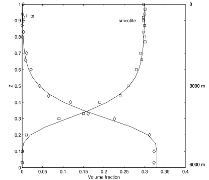
Figure 3:

Figure captions

Figure 1. Comparison of computed porosity (solid curve) with borehole data (depicted as circles) taken from the South China Sea basin. $Z=z/h(t)$ is the scaled height. Compaction in the top region of the basin is essentially at equilibrium (for $\lambda\approx 250,\Xi=2.4,m=8.3,n=1.46,t=7.3$). The porosity profile decreases nearly exponentially.

Figure 2 Temperature profile for $\Lambda=150$ with all other values are the same as in Fig. 1. Numerical simulation (solid curve) is very consistent with the data from Log I.

Figure 3 Comparison of numerical results (solid curves) with data from Log I. The volume fractions of smectite and illite change dramatically in a very thin reaction region. The values used in the simulations are $\lambda=250,\,t=7.3,\,\Theta_{c}=3.4,\,\beta=2.4$.

REFERENCES

Abercrombie, H. J, Hutcheon, I. E., Bloch, J. D. & Caritat, P., 1994, Silica activity and the smectite-illite reaction, Geology, v.22, p.539-542.

Audet, D.M. & Fowler, A.C., 1992. A mathematical model for compaction in sedimentary basins, Geophys. J. Int., 110, 577-590.

Angevine, C. L. & Turcotte, D. L., 1983. Porosity reduction by pressure solution: A theoretical model for quartz arenites, Geol. Soc. Am. Bull., 94, 1129-1134.

Bathurst, R. G. C., 1971. Carbonate sediments and their diagenesis, Elsevier, Amsterdam.

Birchwood, R. A. & Turcotte, D. L., 1994. A unified approach to geopressuring, low-permeability zone formation, and secondary porosity generation in sedimentary basins, J. Geophys. Res., 99, 20051-20058.

Bird, R.B., Armstrong, R.C. & Hassager, O., 1977. Dynamics of polymeric liquids, Vol.1, John Willy & Son press.

Connolly, J.A.D. and Podladchikov, Y. Y., 2000. Temperature-dependent viscoelastic compaction and compartmentalization in sedimentary basins, Tectonophysics, (in press)

Connolly, J. A. D., 1997. Devolatilization-generated fluid pressure and deformation-propagated fluid flow during regional metamorephism., J. Geophys. Res., 102:18149-18173.

Connolly, J.A.D. and Podladchikov, Y. Y., 1998. Compaction-driven fluid flow in viscoelastic rock. Geodinamica Acta, 11:55-85.

Dunnington, H. V., 1954. Stylolite development post-dates rock induration, J. Sedimen. Petrol., 24:27-49

Eberl, D. and Hower, J., 1976, Kinetics of illite formation, Geol. Soc. Am. Bull., v. 87, 1326-1330.

Fowler, A.C., 1990. A compaction model for melt transport in the Earth’s asthenosphere. Part I: the basic model, in Magma Transport and Storage, ed. Ryan, M.P., John Wiley, pp. 3-14.

Fowler, A. C. and Yang, X. S., 1998. Fast and Slow Compaction in Sedimentary Basins, SIAM Jour. Appl. Math., 59, 365-385.

Fowler, A. C. and Yang, X. S., 1999. Pressure Solution and Viscous Compaction in Sedimentary Basins, J. Geophys. Res., B 104, 12 989-12 997.

Fowler, A. C., 2000. Compaction and diagenesis, Proceeding of IMA, (in press)

Fuchs, T., 1894. Über die Natur und Entstehung der Stylolithen, Sitzungsber. Akad. Wiss. Wien. Math-Naturwiss, 103:928-41.

Gibson, R. E., England, G. L. & Hussey, M. J. L., 1967. The theory of one-dimensional consolidation of saturated clays, I. finite non-linear consolidation of thin homogeneous layers, Can. Geotech. J., 17, 261-273.

Heald, M. T., 1955. Stylolites in sandstones, J. Geol., 63:101-114

Hedberg, H.D., 1936. Gravitational compaction of clays and shales, Am. J. Sci., 184, 241-287.

Lerche, I. 1990. Basin analysis: quantitative methods, Vol. I, Academic Press, San Diego, California.

McKenzie, D. P., 1984. The generation and compaction of partial melts, J. Petrol., 25, 713-765.

Meek, P.C. & Norbury, J., 1982. Two-stage, two level finite difference schemes for no-linear parabolic equations, IMA J. Num. Anal., 2, 335-356.

Nield, D. A, 1991. Estimation of the stagnant thermal-conductivity of the saturated porous media, Int. J. Heat. Mass Trans, 34:1575-1576

Patterson, M. S., 1973. Nonhydrostatic thermodynamics and its geological applications, Rev. Geophys. Space Phys., 11, 355-389.

Revil, A. 1999. Pervasive pressure-solution transfer: a poro-visco-plastic model, Geophys. Res. Lett., 26:255-258

item Rimstidt, J. D. & Barnes, H. L., 1980. The kinetics of silica-water reactions, Geochim. Cosmochim. Acta, 44, 1683-1699.

Rieke, H.H. & Chilingarian, C.V., 1974. Compaction of argillaceous sediments, Elsevier, Armsterdam, 474pp.

Rutter, E. H., 1983. Pressure solution in nature, theory and experiment, J. Geol. Soc. London, 140:725-740

Schneider, F., Potdevin, J.L., Wolf, S. and Faille, I. 1996. Mechanical and chemical compaction model for sedimentary basin simulators, Tectonophysics, 263:307-317

Sharp, J. M., 1976. Momentum and energy balance equations for compacting sediments, Math. Geol., 8, 305-332.

Smith, J.E., 1971. The dynamics of shale compaction and evolution in pore-fluid pressures, Math. Geol., 3, 239-263.

Sorby, H. C., 1863. On the direct correlation of mechanical and chemical forces, Proc. R. Soc. London, 12:583-600

Stockdale, P. B., 1922. Stylolites: their nature and origin, Indiana Uni. Stud., 9:1-97

Tada,R. and Siever, R., 1989. Pressure solution during diagenesis, Ann. Rev. Earth. Planet. Sci., 17:89-118.

Velde, B. and Vasseur, G., 1992, Estimation of the diagenetic smectite illite transformation in time-temperature space, Amer. Mineral., v. 77, 967-976.

Wangen, M., 1992. Pressure and temperature evolution in sedimentary basins, Geophys. J. Int., 110, 601-613.

Weyl, P. K., 1959. Pressure solution and the force of crystallization–a phenomenological theory, J. Geophys. Res., 64:2001-2025

Yang, X. S., 2000a. Pressure solution in sedimentary basins: effect of temperature gradient, Earth. Planet. Sci. Lett., 176:233-243

Yang, X. S., 2000b. Modeling mineral reactions in compacting sedimentary basins, Geophys. Res. Lett., 27:1307-1310

Yang, X. S., 2000c. Nonlinear viscoelastic compaction in sedimentary basins, Nonlinear Process Geophys., 7:1-7