The influence of quintessence on the motion of a binary system in cosmology

Abstract

We employ the metric of Schwarzschild space surrounded by quintessential matter to study the trajectories of test masses on the motion of a binary system. The results, which are obtained through the gradually approximate approach, can be used to search for dark energy via the difference of the azimuth angle of the pericenter. The classification of the motion is discussed.

I Introduction

Several astrophysical observational data have shown that our universe is undergoing an era of accelerated expansion trj1 ; trj2 ; trj3 . Therefore, in order to explain this bizarre phenomenon, various models of cosmology have been put forward, ranging from the simplest one of a cosmological constant to the scalar field theory of dark energy and modified gravitational theory as well trj4 ; trj5 ; trj6 . On the other hand, taking dark energy for the presumed cosmological component is also used, combined with the Einstein field equations, to deal with some local gravitational issues trj7 ; trj8 , such as the relevant features of black holes. Recently, Kiselev has brought forward new static spherically symmetric exact solutions of the Einstein equations, either for a charged or uncharged black hole surrounded by quintessential matter or free from it, which satisfy the condition of the additivity and linearity trj9 . Otherwise, using a linear post-Newtonian approach, Kerr et al. considered the orbital differential equations for test bodies of a binary system in the Kerr-de Sitter spacetime and gave the elliptically orbital solution trj10 . The solutions for parabolic and hyperbolic orbits can be obtained via the formulae of trj11 . In this paper, we study the trajectories of test masses in a binary system under the general metric mentioned in trj9 . Four discrete theoretical values of the state parameter $\omega$ from $0$ to $-1$ are used to solve the orbital equations, respectively. Similar to the classic tests of Einstein’s general relativity trj12 , the formulae gotten here can be used to explore whether dark energy exists or not along with the improvement upon observational techniques in astronomy. By introducing the effective potential, we also discuss the classification of the motion. The metric for a black hole surrounded by quintessence is laid out in Section II. We calculate trajectories of test masses in detail in Section III. In Section IV, we display the classification of the motion and a brief conclusion follows. We use the metric signature $(+,-,-,-)$ and make $G$, $\hbar$ and $c$ equal to unity.

II The metric for Schwarzschild space surrounded by the quintessential matter

To begin with, Kiselev’s work trj9 is reviewed briefly. The interval of a spherically symmetric static gravitational field is

$$ds^{2}=e^{\nu}dt^{2}-e^{\mu}dr^{2}-r^{2}\left(d\theta^{2}+\sin^{2}\theta d\varphi^{2}\right),$$ (1)

where $\nu$ and $\mu$ are functions of $r$. Due to the condition of the additivity and linearity, which implies $\mu+\nu=0$, the energy-momentum tensor of quintessence can be written as

$${T_{t}}^{t}={T_{r}}^{r}=\rho_{q},$$ (2)

$${T_{\theta}}^{\theta}={T_{\varphi}}^{\varphi}=-\frac{1}{2}\,\rho_{q}\,(3\omega+1),$$ (3)

where $\rho_{q}$ is the density of the quintessential matter while $\omega$ is the state parameter. By setting $\mu=-\ln(1+f)$, we get

$$r^{2}f^{\prime\prime}+3(1+\omega)\,rf^{\prime}+(3\omega+1)f=0,$$ (4)

whose solutions are of the forms

$$f_{q}=\frac{\lambda}{r^{3\omega+1}},$$ (5)

$$f_{\emph{BH}}=-\frac{r_{\textsl{g}}}{r},$$ (6)

where $\lambda$ and $r_{\textsl{g}}$ are the normalization factors. Then, according to the relation

$$\rho_{q}=\frac{\lambda}{2}\,\frac{3\omega}{r^{3(1+\omega)}},$$ (7)

$\lambda$ should be negative for quintessence because the density of energy is positive. As a resulting, the metric for the space surrounded by the quintessential matter can be expressed by

$$ds^{2}=\left(1-\frac{2M}{r}-\frac{\lambda}{r^{3\omega+1}}\right)dt^{2}-\left(1-\frac{2M}{r}-\frac{\lambda}{r^{3\omega+1}}\right)^{-1}dr^{2}-r^{2}\left(d\theta^{2}+\sin^{2}\theta d\varphi^{2}\right),$$ (8)

where $M$ is the black hole mass and $r_{\textsl{g}}=2M$. Obviously, it can be reduced to the Schwarzschild and Schwarzschild-de Sitter metrics by $\lambda=0$ and $\omega=-1$, respectively.

III Trajectory of the test mass and the motion of a binary system

In relativistic dynamics, the contravariant 4D momentum $p^{\mu}$ is defined as $p^{\mu}=m\frac{dx^{\mu}}{d\tau}$, where $m$ is the rest mass. Then the covariant momentum, which is more important in dynamics, can be introduced by $p_{\mu}=\textsl{g}_{\mu\nu}p^{\nu}$. When particles move in the gravitational field, dynamical conserved quantities are determined by the space-time symmetry of the metric field. From the metric (8), we may see clearly that $t$ and $\varphi$ are both cyclic coordinates; therefore, conserved quantities of the test mass are the $t$ and $\varphi$ components of $p_{\mu}$, i.e.

$$p_{0}=m\left(1-\frac{2M}{r}-\frac{\lambda}{r^{3\omega+1}}\right)\frac{dt}{d\tau}=\mbox{const.},$$ (9)

$$p_{3}=-mr^{2}\sin^{2}\theta\frac{d\varphi}{d\tau}=\mbox{const.}.$$ (10)

Due to the symmetry, the test mass moves on the symmetric plane formed by the initial velocity vector (3D) and center of force. We regard the direction vertical to the orbital plane as the polar axis. Then the motion of the test mass satisfies

$$\theta=\frac{\pi}{2},\ \ \ \ \frac{d\theta}{d\tau}=0.$$ (11)

$p_{0}$ and $p_{3}$ are conserved quantities written in the form

$$\left(1-\frac{2M}{r}-\frac{\lambda}{r^{3\omega+1}}\right)\frac{dt}{d\tau}=E,$$ (12)

$$r^{2}\frac{d\varphi}{d\tau}=L,$$ (13)

where $E$ and $L$ are constants of integration that represent energy and angular momentum per unit mass, respectively. Furthermore, the normalization condition for the 4D velocity, $\textsl{g}_{\mu\nu}u^{\mu}u^{\nu}=1$, also provides the equation

$$\left(1-\frac{2M}{r}-\frac{\lambda}{r^{3\omega+1}}\right)\left(\frac{dt}{d\tau}\right)^{2}-\left(1-\frac{2M}{r}-\frac{\lambda}{r^{3\omega+1}}\right)^{-1}\left(\frac{dr}{d\tau}\right)^{2}-r^{2}\left(\frac{d\varphi}{d\tau}\right)^{2}=1.$$ (14)

Equations (11) to (14) are four first integrals of the geodesic equation, which compose a set of self-contained differential equations of particle dynamics.

After being cleared up, these equations can lead to the relativistic extension of the Binet formula of Newtonian mechanics,

$$\frac{d^{2}u}{d\varphi^{2}}+u=\frac{M}{L^{2}}+3Mu^{2}+\frac{\lambda\left(3\omega+1\right)}{2L^{2}}u^{3\omega}+\frac{\lambda\left(3\omega+3\right)}{2}u^{3\omega+2},$$ (15)

where $\frac{dr}{d\varphi}\neq 0$, because the orbit is not a circle and the second term on the right-hand side is a relativistic correction, while the last two are quintessential contributions. We have introduced the dimensionless variable $u=GM/r$, and for convenience $u=1/r$ has been used in the process of the calculation.

Note that $u=GM/r$ is a small quantity. When $\omega<0$, $u$ also appears in the denominator. So we now evaluate the magnitude of the last two terms of Eq. (15). First, we make the transformation $\alpha=-3\omega$ and $\beta=\lambda^{1/\alpha}$; then Eq. (15) turns to

$$\frac{d^{2}u}{d\varphi^{2}}+u=\frac{M}{L^{2}}+3Mu^{2}+\frac{1-\alpha}{2L^{2}}\left(\frac{\beta}{u}\right)^{\alpha}+\frac{3-\alpha}{2}\left(\frac{\beta}{u}\right)^{\alpha}u^{2}.$$ (16)

The transformation parameter $\alpha$ satisfies $\alpha\in[0,3]$, while $\omega\in[-1,0]$. As for $\beta$, we know that the state parameter $\omega=-1$ represents the standard $\Lambda\textrm{CDM}$ model, and therefore $\beta\sim\Lambda^{1/3}$. From recent cosmological observations, the magnitude of the cosmological constant is $\Lambda\approx{H_{0}}^{2}/c^{2}\approx 10^{-52}\,\textrm{m}^{-2}$ with $H_{0}\approx 70\,\textrm{km}\,\textrm{s}^{-1}\,\textrm{Mpc}^{-1}$. As a result, the magnitude of $\beta$ is $\beta\sim(10^{-52})^{1/3}<10^{-17}$. Furthermore, due to the definition $u=GM/r$, we have the expression

$$\frac{\beta}{u}=\frac{\beta r}{GM}.$$ (17)

By way of a practical evaluation, we take the orbital radius of Mercury, $r=5\times 10^{10}\,\textrm{m}$, which is the smallest in the solar system and for the other parameters we get $GM=1.5\times 10^{3}\,\textrm{m}$. As a result, Eq. (17) yields

$$\frac{\beta}{u}\approx\frac{10^{-17}\times 5\times 10^{-10}}{1.5\times 10^{3}}\approx 3.3\times 10^{-10}\ll u\sim 10^{-7}.$$ (18)

Furthermore, from the Binet equation in Newtonian mechanics,

$$\frac{d^{2}u}{d\varphi^{2}}+u=\frac{M}{L^{2}},$$ (19)

whose solution is

$$u(\varphi)=\frac{M}{L^{2}}(1+e\cos\varphi),$$ (20)

we find that $M/L^{2}\sim u$. Therefore, when $\alpha>0\,(\omega<0)$ the last two terms of Eq. (15) are far less than $u$ and $M/L^{2}$ and can be regarded as small corrections.

According to the linear perturbation scheme put forward in trj10 , the last three terms could be treated as perturbations being a function of $\varphi$ by substituting for $u$ the unperturbed solution. Due to the supernova’s dimming, the dark energy should satisfy $\omega\leq-2/3$ to fit the observations trj13 ; trj14 . But here, without essential loss of generality, we evaluate the quintessential matter from a theoretical point of view with the state parameter in the range of $\omega\in[-1,0]$. So we discuss the influence of quintessence on the trajectory of the test mass in four cases.

III.1 case of $\omega=0$

When $\omega=0$, Eq. (15) reduces to

$$\frac{d^{2}u}{d\varphi^{2}}+u=\frac{M+\frac{\lambda}{2}}{L^{2}}+\left(3M+\frac{3\lambda}{2}\right)u^{2},$$ (21)

where $u$ is a small quantity, resulting in a slight correction of $u^{2}$. So we ignore it in the first place, and we find the zeroth-order approximate solution

$$u_{0}=\frac{M+\frac{\lambda}{2}}{L^{2}}\left(1+e\cos\varphi\right).$$ (22)

We presume that the bound orbit is an ellipse with eccentricity $e<1$. Via substituting $u_{0}$ into the right-hand side of Eq. (21), we can get the first-order approximate solution

$$u=\left(\frac{M+\frac{\lambda}{2}}{L^{2}}\right)\left[1+e\cos\varphi+3\left(M+\frac{\lambda}{2}\right)\left(\frac{M+\frac{\lambda}{2}}{L^{2}}\right)e\varphi\sin\varphi\right],$$ (23)

where small higher-order quantities, which are impossible to measure very accurately, are neglected for their insignificant effects. Furthermore, Eq. (22) means that $(M+\frac{\lambda}{2})/L^{2}\sim u$, and in the weak-field regime, $M\ll r$. Introducing $\varepsilon\equiv 3(M+\frac{\lambda}{2})[(M+\frac{\lambda}{2})/L^{2}]$, namely $\varepsilon\ll 1$, makes $\cos\varepsilon\varphi\sim 1$ and $\sin\varepsilon\varphi\sim\varepsilon\varphi$. Then Eq. (23) reduces to

$$u\left(\varphi\right)\approx\left(\frac{M+\frac{\lambda}{2}}{L^{2}}\right)\left[1+e\cos\left(1-\varepsilon\right)\varphi\right].$$ (24)

When considering precession, we may get the difference of the azimuth angle of the pericenter

$$\triangle\varphi=6\pi\left(\frac{M}{L}\right)^{2}+6\pi\left(\frac{\lambda M+\lambda^{2}/4}{L^{2}}\right),$$ (25)

where we ignore a quantity of $\varepsilon^{2}$, and the second term on the right-hand side belongs to quintessence.

III.2 case of $\omega=-1/3$

When $\omega=-1/3$, Eq. (15) reduces to

$$\frac{d^{2}u}{d\varphi^{2}}+\left(1-\lambda\right)u=\frac{M}{L^{2}}+3Mu^{2}.$$ (26)

Similar to the case of $\omega=0$, the zeroth-order approximate solution is

$$u_{0}=\frac{M}{L^{2}}\left[1+e\cos\left(\varphi\sqrt{1-\lambda}\right)\right];$$ (27)

then the first-order approximate solution reads

$$u=\frac{M}{L^{2}}\left[1+e\cos\left(\varphi\sqrt{1-\lambda}\right)+\frac{3M^{2}}{L^{2}\sqrt{1-\lambda}}e\varphi\sin\left(\varphi\sqrt{1-\lambda}\right)\right].$$ (28)

Introducing $\varepsilon\equiv\frac{3M^{2}}{L^{2}\sqrt{1-\lambda}}$ makes Eq. (28) reduce to

$$u\left(\varphi\right)=\frac{M}{L^{2}}\left\{1+e\cos\left[\left(\sqrt{1-\lambda}-\varepsilon\right)\varphi\right]\right\}.$$ (29)

Furthermore, the difference of the azimuth angle is

$$\triangle\varphi=6\pi\frac{M^{2}}{L^{2}\left(1-\lambda\right)^{3/2}}+2\pi\left(\frac{1-\sqrt{1-\lambda}}{\sqrt{1-\lambda}}\right).$$ (30)

Here, $\varepsilon^{2}$ is ignored, and quintessence also affects the first term, because the zeroth-order approximate solution is changed for the component $\varphi$.

III.3 case of $\omega=-2/3$

When $\omega=-2/3$, Eq. (15) reduces to

$$\frac{d^{2}u}{d\varphi^{2}}+u=\left(\frac{M}{L^{2}}+\frac{\lambda}{2}\right)+3Mu^{2}-\frac{\lambda}{2L^{2}u^{2}}.$$ (31)

Obviously, the form turns out to be complicated, because $u^{2}$ appears in the denominator. But as mentioned before, $\lambda\sim\Lambda$, so the last two terms are both perturbation ones. Here we could deal with it by the linear perturbation scheme in trj10 , where the motion of test bodies in the Kerr-de Sitter spacetime was studied. Substituting the zeroth-order approximate solution $u_{0}=\frac{1}{p}\left(1+e\cos\varphi\right)$ with $p=\left(\frac{M}{L^{2}}+\frac{\lambda}{2}\right)^{-1}$ for $u$ into the r.h.s. of Eq. (31), we can divide the resulting linear equation into two parts:

$$\frac{d^{2}u_{1}}{d\varphi^{2}}+u_{1}=3Mp^{-2}\left(1+e\cos\varphi\right)^{2},$$ (32)

$$\frac{d^{2}u_{2}}{d\varphi^{2}}+u_{2}=p^{-1}-\frac{\lambda p^{2}}{2L^{2}\left(1+e\cos\varphi\right)^{2}}.$$ (33)

After being transformed, Eq. (33) can be integrated once to the form

$$\frac{d}{d\xi}\left[\left(1-\xi^{2}\right)^{-\frac{1}{2}}U\right]=-\frac{q}{e\left(1-\xi^{2}\right)^{3/2}\left(1+e\xi\right)}+\frac{C}{\left(1-\xi^{2}\right)^{3/2}},$$ (34)

where $\xi=\cos\varphi$, $U=u_{2}-p^{-1}$, $q=-\frac{\lambda p^{2}}{2L^{2}}$ and $C$ is a constant of integration. If once more we integrate it, using formulae (2.264), (2.266) and (2.269) given in trj15 , then we get

$$U=\frac{q}{1-e^{2}}\left[\left(1+e\Psi\sin\varphi\right)-\frac{1}{e}\cos\varphi\right]+C\cos\varphi+S\sin\varphi,$$ (35)

where $S$ is a constant of integration and

$$\Psi=\frac{1}{\sqrt{1-e^{2}}}\arcsin\left(\frac{e+\cos\varphi}{1+e\cos\varphi}\right).$$ (36)

Combining with a particular solution of Eq. (32), the final solution for this case is $u=U+p^{-1}+3Mp^{-2}e\varphi\sin\varphi$, which can be rewritten in the form

$$u\left(\varphi\right)\approx\frac{q}{1-e^{2}}\left[\left(1+e\Psi\sin\varphi\right)-\frac{1}{e}\cos\varphi\right]+\left(\frac{M}{L^{2}}+\frac{\lambda}{2}\right)\left\{1+e\cos\left[\left(1-\varepsilon\right)\varphi\right]\right\},$$ (37)

with $\varepsilon\equiv 3M\left(\frac{M}{L^{2}}+\frac{\lambda}{2}\right)$ introduced. Here $u$ may reduce to the result of Schwarzschild case trj16 as $\lambda\rightarrow 0$.

III.4 case of $\omega=-1$

When $\omega=-1$, Eq. (15) reduces to

$$\frac{d^{2}u}{d\varphi^{2}}+u=\frac{M}{L^{2}}+3Mu^{2}-\frac{\lambda}{L^{2}u^{3}}.$$ (38)

The unperturbed solution is $u_{0}=\frac{1}{p}\left(1+e\cos\varphi\right)$ with $p=\left(\frac{M}{L^{2}}\right)^{-1}$. Similar to the case of $\omega=-2/3$, according to the result (49) in trj10 the approximate solution is

$$u\left(\varphi\right)\approx\frac{q}{2\left(1-e^{2}\right)^{2}}\left[3\left(1+e\Psi\sin\varphi\right)-\frac{1-e^{2}}{1+e\cos\varphi}-\left(2e+\frac{1}{e}\right)\cos\varphi\right]+\frac{M}{L^{2}}\left\{1+e\cos\left[\left(1-\varepsilon\right)\varphi\right]\right\},$$ (39)

where $q=-\lambda p^{3}/L^{2}$, $\varepsilon\equiv 3M^{2}/L^{2}$ and $\Psi$ is represented by Eq. (36). When $\lambda\rightarrow 0$, this result reduces to the Schwarzschild solution. It is different from the two former cases in that the difference of the azimuth angle of the pericenter hardly comes out when $\omega=-2/3$ or $-1$ due to the complicated form.

IV Discussion and conclusion

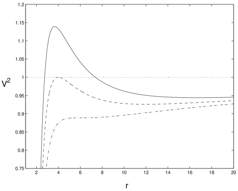
Figure 1: The effective potential $V^{2}$ for timelike geodesics for variable $L$ with $\lambda=0$ and $M=1$. Solid line for $L>4$, dash line for $L=4$, dash-dot line for $L=2\sqrt{3}$.

Here, we turn to a discussion of the classification of the motion. First, we introduce the relativistic effective potential

$$V^{2}=\left(1-\frac{2M}{r}-\frac{\lambda}{r^{3\omega+1}}\right)\left(1+\frac{L^{2}}{r^{2}}\right).$$ (40)

Thus, the radial equation derived from (14) can be rewritten as $\left(\frac{dr}{d\tau}\right)^{2}=E^{2}-V^{2}$, which implies that the possible motions only occur when $E^{2}\geqslant V^{2}$. Expand Eq. (40),

$$V^{2}=1-\frac{2M}{r}+\frac{L^{2}}{r^{2}}-\frac{2ML^{2}}{r^{3}}-\frac{\lambda}{r^{3\omega+1}}-\frac{\lambda L^{2}}{r^{3\omega+3}}.$$ (41)

Because the effect of $\lambda$ on $V^{2}$ is very small, the curves of $V^{2}$ are almost the same as that in the Schwarzschild space trj16 . So we illustrate the effective potential $V^{2}$ for variable $L$ with $\lambda=0$ in Fig. 1.

From Fig. 1, we see that for $L>4$, there is a potential barrier whose peak value is larger than 1 when $r$ is very small, while there is also a potential well when $r$ is large. Thus, the possible motions can be classified as three kinds

$$E^{2}<1,\ \ \ \ \ \ \ \ \ \ \ \ \ \ \ \ \ \ \ \text{the bound state};$$

$$1\leqslant E^{2}<V_{\textrm{max}}^{2},\ \ \ \ \text{the scattering state};$$

$$E^{2}\geqslant V_{\textrm{max}}^{2},\ \ \ \ \ \ \ \ \ \ \ \text{the absorbing state}.$$

With decreasing $L$, the central potential barrier decreases in altitude. In the range of $2\sqrt{3}\leqslant L\leqslant 4$, $V_{\textrm{max}}^{2}\leqslant 1$, which indicates that the appearance of the scattering state is impossible, with the bound and absorbing states being left over. If $L<2\sqrt{3}$, both the peak and the hollow of the effective potential will disappear, and only the absorbing state is left over. But note that the above analysis is based on one assumption that the radius of the gravitation source is so small that the exterior of the source is applicable for very small $r$.

In summary, we have studied the trajectories of test bodies on the motion of a binary system in the presence of quintessence. There are four cases of the state parameter $\omega$ of quintessence, and we obtain four corresponding orbital equations, where it is assumed that the test mass moves round the center of force with eccentricity $e<1$. The difference of the azimuth angle of the pericenter can be cast in formulae in the two former cases, while the other two complicated ones can hardly be done, considering their different forms. Moreover, the effect caused by dark energy is too small to be detectable in the solar system. But the common feature of our four cases is that the resultant solutions reduce to the outcomes in Schwarzschild space naturally as the parameter $\lambda$ vanishes.

- (1) A.G. Riess, et al., Astron. J. 116 (1998) 1009, astro-ph/9805201.
- (2) S. Perlmutter, et al., Astrophys. J. 517 (1999) 565, astro-ph/9812133.
- (3) S. Perlmutter, et al., Astrophys. J. 598 (2003) 102.
- (4) P.J.E. Peebles, B. Ratra, Rev. Mod. Phys. 75 (2003) 559-606, astro-ph/0207347.
- (5) V. Sahni, Lect. Notes Phys. 653 (2004) 141-180, astro-ph/0403324.
- (6) T. Padmanabhan, Phys. Rep. 380 (2003) 235.
- (7) K. Lake, Phys. Rev. D 65 (2002) 087301, gr-qc/0103057.
- (8) V. Kagramanova, J. Kunz, C. Lämmerzahl, Phys. Lett. B 634 (2006) 465-470, gr-qc/0602002.
- (9) V.V. Kiselev, Class. Quant. Grav. 20 (2003) 1187-1198, gr-qc/0210040.
- (10) A.W. Kerr, J.C. Hauck, B. Mashhoon, Class. Quant. Grav. 20 (2003) 2727, gr-qc/0301057.
- (11) J.M.A. Danby, Fundamentals of celestial mechanics 2nd edn, Willmann-Bell, Richmond (1988).
- (12) S. Weinberg, Gravitation and cosmology, John Wilcy & Sons, Inc., New York, Sect. 8 (1972).
- (13) P.S. Corasaniti, E.J. Copeland, Phys. Rev. D 65 (2002) 043004.
- (14) M. Tegmark, et al. [SDSS Collaboration], Phys. Rev. D 69 (2004) 103501.
- (15) I.S. Gradshteyn and I.M. Ryzhik, Table of integrals, series, and products, Academic Press, Inc., New York (1980).
- (16) R.M. Wald, General relativity, The University of Chicago, Chicago (1984).