Dynamics of Periodically-kicked Oscillators

Abstract

We review some recent results surrounding a general mechanism for producing chaotic behavior in periodically-kicked oscillators. The key geometric ideas are illustrated via a simple linear shear model.

Dedicated to Steve Smale on the occasion of his 80th birthday

Introduction

This paper reviews some recent results on a topic with a considerable history: the periodic forcing of limit cycles. Some 80 years ago, van der Pol and van der Mark observed that irregularities developed when certain electrical circuits exhibiting stable oscillations were periodically forced [26]. Their work stimulated a number of analytical studies; see e.g. [5, 13, 12, 9]. Another classical example of driven oscillators is the FitzHugh-Nagumo neuron model [6]; the response of this and other models of biological rhythms to external perturbations have been extensively studied (see e.g. [33]). As a topic of mathematical study, the dynamics of forced oscillations is well motivated: Oscillatory behavior are ubiquitous in physical, biological, and engineered systems, and external forcing, whether artificially applied or as a way to model forces not intrinsic to the system, is also commonplace.

In this article, we are not concerned with modeling specific physical phenomena. Instead, we consider a generic dynamical system with a limit cycle, and seek to understand its qualitative behavior when the system is periodically disturbed. To limit the scope of the problem, we restrict ourselves to periodic kicks, or forcings that are turned on for only short durations, leaving the limit cycle ample time to restore itself during the relaxation period. We are interested in large-time behavior, particularly in questions of stability and chaos.

As we will show, one of the properties of the limit cycle that plays a key role in determining whether the kicked system is stable or chaotic is shear, by which we refer to the differential in speed (or angular velocity) for orbits near the limit cycle. A central theme of this article is that under suitable conditions, the impact of a kick can be substantially magnified by the underlying shear in the unforced system, leading to the formation of horseshoes and strange attractors. This does not always happen, however: some limit cycles are more vulnerable, and some types of kicks are more effective than others. These ideas are discussed in [29, 30] and [14], the material which forms the basis of the present review.

Even though we seek to provide insight into dynamical mechanisms that operate under general conditions, we have found the ideas to be most transparent in a very simple linear shear model, to which we will devote a nontrivial part of the paper. Sect. 1 introduces this example and familiarizes the reader with the various parameters (including the one which measures shear); it also reports on results of a numerical study on Lyapunov exponents. Sects. 2 and 3 are organized around explaining these simulation results. Along the way, we take the opportunity to review a number of mathematical ideas which clearly go beyond this one example. Some of the rigorous results reviewed, notably those on SRB measures for a relevant class of strange attractors [28, 31, 32], are recent developments. With the main ingredients of the linear shear model and the relevant mathematical background in hand, we return to a discussion of general limit cycles in the final section.

1 Increasing Shear as a Route to Chaos

This section introduces the main example we use in this review, and acquaints the reader with the various parameters in the model and how they impact the dynamics. Of particular interest to us is the effect of increasing shear. Numerically computed Lyapunov exponents as functions of shear are presented in Sect. 1.3. They will serve as a focal point for some discussions to follow.

1.1 Periodic kicking of linear shear flow

Our main example is the periodic kicking of a linear shear flow with a hyperbolic limit cycle. This 2D model was studied rigorously in [29, 30] and numerically in [14, 35]. Though exceedingly simple in appearance, it already exhibits rich and complex dynamical behaviors.

The model is given by

$$\begin{array}[]{ccl}\dot{\theta}&=&1+\sigma y\ ,\\[4.30554pt] \dot{y}&=&-\lambda y~{}+~{}A\cdot\sin(2\pi\theta)\cdot\sum_{n=-\infty}^{\infty}\delta(t-n\tau)\ ,\\ \end{array}$$ (1)

where $(\theta,y)\in{\mathbb{S}}^{1}\times{\mathbb{R}}$, ${\mathbb{S}}^{1}\equiv{\mathbb{R}}/{\mathbb{Z}}$, and $\sigma,\lambda,A$ and $\tau$ are constants with $\sigma,\lambda,\tau>0$. We will refer to Eq. (1) with $A=0$ as the unforced equation, and the term involving $A$ as the forcing or the kick. Here $\delta$ is the usual $\delta$-function, that is to say, the kicks occur instantaneously at times $0,\tau,2\tau,3\tau,\dots$.

More precisely, let $\Phi_{t}$ denote the flow corresponding to the unforced equation. It is easy to see that for all $z\in{\mathbb{S}}^{1}\times{\mathbb{R}}$, $\Phi_{t}(z)$ tends to the limit cycle $\gamma=\{y=0\}$ as $t\to\infty$. The precise meaning of Eq. (1) is as follows: Let $\kappa(\theta,y)=(\theta,y+A\sin(2\pi\theta))$ be the kick map; it represents the action of the forcing term. Then assuming we start with a kick at time $0$, the time-$\tau$ map of the flow generated by Eq. (1) is

$$\Psi_{\tau}=\Phi_{\tau}\circ\kappa,$$

and the evolution of the system is defined by iterating $\Psi_{\tau}$. We generally assume that $\tau$ is not too small, so that during the relaxation period between kicks, the flow $\Phi_{t}$ of the unforced equation “restores” the system to some degree.

The parameters of interest are:

$$\sigma =\mbox{amount of shear,}$$

$$\lambda =\mbox{rate of contraction to $\gamma$,}$$

$$A =\mbox{amplitude of kicks, and}$$

$$\tau =\mbox{time interval between kicks.}$$

Our aim in the remainder of this section is to understand – via geometric reasoning and numerical simulations – the meanings of these quantities, and the roles they play in questions of stability and chaos. Our line of reasoning follows [29] and [14].

1.2 Geometry of $\Psi_{\tau}$

A simple way to gain intuition on the geometry of $\Psi_{\tau}$ is to study the $\Psi_{\tau}$-image of $\gamma$, the limit cycle of the unforced system. We will do so by freezing some of the parameters and varying others.

Effects of varying $\sigma,\lambda$, and $A$

To begin with, let us freeze $\lambda,$ $A,$ and $\tau$. To fix ideas, let us take $\lambda$ to be relatively small, so that the rate of contraction is weak, and choose $\tau$ large enough that $e^{-\lambda\tau}$ is a nontrivial contraction. This is when the effects of shear are seen most clearly. In Fig. 1, $\lambda=A=0.1$, and $\tau=10$. Here $\Psi_{\tau}(0,0)=(0,0)$ because the limit cycle $\gamma$ has period $1$ and $\tau$ is an integer multiple of this period; for non-integer $\tau$ the picture is shifted horizontally.

Fig. 1(b) shows four images of $\gamma$ under $\Psi_{\tau}$ for increasing shear. The larger $\sigma$, the greater the difference in velocity between two points with different $y$ coordinates. This applies in particular to the highest and lowest points in $\kappa(\gamma)$ in Fig. 1(a). For $\sigma$ small enough, order in the $\theta$-direction is preserved, i.e., for $z_{1}=(\theta_{1},0)$ and $z_{2}=(\theta_{1}+\varepsilon,0)$, $\Psi_{\tau}(z_{1})$ will continue to have a slightly smaller $\theta$-coordinate than $\Psi_{\tau}(z_{2})$. As $\sigma$ increases, some points in $\gamma$ may “overtake” others, spoiling this order. As $\sigma$ gets larger still, the total distances traveled in $\tau$ units of time vary even more, and a fold develops. This fold can be made arbitrarily large: we can make it wrap around the cylinder as many times as we wish by taking $\sigma$ large enough.

$y$

(a) The limit cycle $\gamma$ and its image $\kappa(\gamma)$ after one kick

$\sigma=0.05$		$\sigma=0.25$
$\sigma=0.5$		$\sigma=1$

(b) $\Psi_{\tau}(\gamma)$ for $\tau=10$

Figure 1: Effect of increasing shear. Here, $\lambda=A=0.1$.

If we had fixed $\sigma$ instead, and increased $\lambda$ starting from $\lambda=0.1$, the resulting sequence of pictures would be qualitatively similar to Fig. 1(b) but in reverse order: The smallest $\lambda$ would correspond to the bottom-right image in Fig. 1(b), and the largest $\lambda$ to the top-left — provided $\tau$ is scaled so that $\lambda\tau$ remains constant. This is because for $\lambda$ small, $\kappa(\gamma)$ returns to $\gamma$ very slowly, giving the shear a great deal of time to act, while for larger $\lambda$, $\kappa(\gamma)$ is brought back to $\gamma$ more quickly. Thus all else being equal, $\sigma$ and $\lambda$, i.e., shear and damping, have opposite effects.

The consequence of varying $A$ while keeping the other parameters fixed is easy to see: the stronger the kick, the greater the difference in $y$-coordinate between the highest and lowest points in $\kappa(\gamma)$, and the farther apart their $\theta$-coordinates will be when flowed forward by $\Phi_{\tau}$.

What we learn from the sequence in snapshots in Fig. 1 is that $A$ acts in concert with $\sigma$ to promote fold creation, while $\lambda$ works against it.

Formulas for $\Psi_{\tau}$

Since the unforced equation is easy to solve, one can in fact write down explicitly the formulas for $\Psi_{\tau}$. Let $(\theta_{\tau},y_{\tau})=\Psi_{\tau}(\theta_{0},y_{0})$. A simple computation gives

$$\begin{array}[]{rcl}\theta_{\tau}&=&\theta_{0}+\tau+\frac{\sigma}{\lambda}\cdot[y_{0}+A\sin(2\pi\theta_{0})]\cdot(1-e^{-\lambda\tau})\qquad\mbox{(mod 1)}\ ,\\[12.0pt] y_{\tau}&=&e^{-\lambda\tau}[y_{0}+A\sin(2\pi\theta_{0})]\ .\end{array}$$ (2)

The reader can easily check that Eq. (2) is in agreement with the intuition from earlier.

Note the appearance of the ratio $\frac{\sigma}{\lambda}A$, or rather $\frac{\sigma A}{\lambda}(1-e^{-\lambda\tau})$, in the nonlinear term in the equation for $\theta_{\tau}$: the size of this term is a measure of the tendency for a fold to develop in $\Psi_{\tau}(\gamma)$. As is well known to be the case, stretch-and-fold is a standard mechanism for producing chaos. One can, therefore, think of the ratio

$$\frac{\sigma}{\lambda}A\ =\ \frac{\rm shear}{\rm contraction}\cdot{\rm kick\ amplitude}$$

as the key to determining whether the system is chaotic, provided $\lambda\tau$ is large enough that the factor $1-e^{-\lambda\tau}$ is not far from $1$.

Trapping region and attractor

From the above, it is evident that much of the action takes place in a neighborhood around $\gamma.$ Let ${U}=\{|y|\leq A(e^{\lambda\tau}-1)^{-1}\}$, so that $\Psi_{\tau}({U})\subset{U}$, and define

$$\Gamma=\cap_{n\geq 0}\Psi_{\tau}^{n}({U})$$

to be the attractor for the system Eq. (1). The basin of attraction of $\Gamma$ is the entire cylinder $\mathbb{S}^{1}\times\mathbb{R}$, since every orbit will eventually enter $U$. This usage of the word “attractor” implies no knowledge of dynamical indecomposability (a condition required by some authors).

1.3 Lyapunov exponents

Another measure of chaos is orbital instability, or the speed at which nearby orbits diverge. In this subsection, we focus on the larger of the two Lyapunov exponents of $\Psi_{\tau}$, defined to be

$$\Lambda_{\max}(z)\ =\ \lim_{n\to\infty}\frac{1}{n}\log\|D\Psi^{n}_{\tau}(z)\|\ =\ \sup_{v\neq 0}\ \lim_{n\to\infty}\frac{1}{n}\log\|D\Psi^{n}_{\tau}(z)\cdot v\|\ .$$

Leaving technical considerations for later (see Sect. 3.1), we compute numerically $\Lambda_{\max}$ for the systems in question, sampling at various points $z\in{U}$. Notice that $\Lambda_{\max}$ measures the rate of divergence of nearby orbits per kick, not per unit time.

Each of the plots in Fig. 2 shows $\Lambda_{\max}$ as a function of $\tau$ for the values of $\sigma,\lambda$ and $A$ specified. In all six plots, we have fixed $\lambda=A=0.1$, while $\sigma$ varies from plot to plot. The first 4 values of $\sigma$ used in Fig. 2 are the same as those used in Fig. 1(b). In each plot, 10 randomly chosen initial conditions are used, the largest and smallest computed values of $\Lambda_{\max}$ are discarded, and the largest and smallest of the remaining 8 values are shown, the smallest as a solid black dot, and the largest, if visibly different than the smallest, as an open square. The plots show $\tau\in[5,15]$. We give some idea of the rates of contraction and sizes of the trapping regions ${U}$ for these parameters: at $\tau=5$, $e^{-\lambda\tau}=e^{-0.5}\approx 0.61$, and ${U}=\{|y|\lesssim 0.15\}$; at $\tau=15$, $e^{-\lambda\tau}=e^{-1.5}\approx 0.22$, and ${U}=\{|y|\lesssim 0.03\}$.

(a) $\sigma=0.05$		(b) $\sigma=0.25$
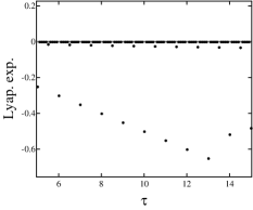
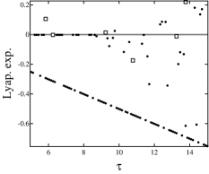
(c) $\sigma=0.5$		(d) $\sigma=1$
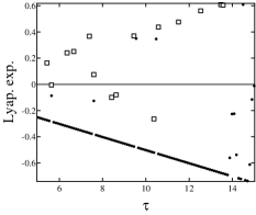
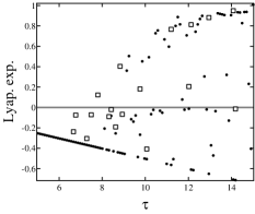
(e) $\sigma=2$		(f) $\sigma=4$

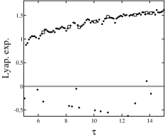
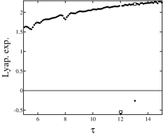
Figure 2: Lyapunov exponents $\Lambda_{\max}$ as functions of kick period $\tau$ for increasing shear $\sigma.$ The other parameters are $\lambda=A=0.1.$ For each $(\sigma,\tau)$, we simulate 10 orbits with random initial conditions, iterating each for $4\times 10^{6}$ steps. We then drop the outliers and plot the remaining estimates, as described in the text.

Observations from simulation results

The discussion in Sect. 1.2 suggests that as shear is increased with other parameters fixed, the system is likely to get increasingly chaotic. This may lead us to expect $\Lambda_{\max}$ to increase monotonically with $\sigma$. As one can see, that may be correct as an overall trend, but the situation is somewhat more complicated:

In the two low-shear regimes, namely $\sigma=0.05$ and $0.25$, with a few exceptions the computed values of $\Lambda_{\max}$ are either zero or negative, with a majority of them at or very near zero for $\sigma=0.05$ and becoming considerably more negative at $\sigma=0.25$. That is to say, $\Lambda_{\max}$ decreases as $\sigma$ increases. Notice that $\Lambda_{\max}<0$ means the trajectory tends to a sink, i.e., a stable fixed point or periodic orbit.

Increasing shear, we see in the middle row of Fig. 2 that at first sinks dominate the landscape, giving way to more instances of positive Lyapunov exponents, i.e., chaotic behavior, as $\sigma$ increases. At $\sigma=1$, the picture is very mixed, with $\Lambda_{\max}$ fluctuating wildly between positive and negative values as $\tau$ varies. Notice also the nontrivial number of open squares, telling us that these parameters often support more than one type of dynamical behavior.

In the two higher-shear regimes, $\sigma=2$ and $4$, $\Lambda_{\max}$ becomes more solidly positive, though occasional sinks are still observed. The route has been a messy one, but one could say that the transition to chaos is complete.

As to the dependence on $\tau$, it appears that other things being equal, longer relaxation times between kicks allow the dynamical phenomenon in effect to play out more completely: regardless of the sign of $\Lambda_{\max}$, its magnitude increases with $\tau$ in each of the plots.

Finally, it is important to remember that the limit cycles used to produce the results in Fig. 2 are weakly attracting, making them more vulnerable to the effects of shear. Strongly attracting limit cycles are more robust, and larger kicks and/or shear will be needed to produce chaos.

In Sects. 2 and 3 we review some rigorous theory that supports the numerically computed values of $\Lambda_{\max}$ shown. To avoid technical assumptions, we will focus on the model in Sect. 1.1, leaving generalizations to Sect. 4. As the reader will see, the mathematical ideas go considerably beyond this one example. On the other hand, even for this simple model, state-of-the-art understanding is incomplete. In the next two sections, we will vary $\sigma,\lambda,A$ and $\tau$, and show that there are regions in the parameter space for which a clear description of the dynamics is available, and larger regions on which there is partial understanding.

2 Geometric Structures

To analyze a dynamical system, it is often useful to begin by identifying its most prominent structures, those that are a significant part of the landscape. Even when they do not tell the whole story, these structures will serve as points of reference from which to explore the phase space. This section describes structures of this type for the systems defined by Eq. (1).

2.1 Persistence of limit cycles at very low shear

Proposition 2.1 ([29])

Given $\lambda\tau>0$, the following hold for $\frac{\sigma}{\lambda}$ and $A$ sufficiently small:

(a) the attractor $\Gamma$ is a smooth, closed invariant curve near $\gamma$;

(b) every $\zeta\in{\mathbb{S}}^{1}\times{\mathbb{R}}$ lies in the strong stable curve $W_{\Psi_{\tau}}^{ss}(z)$ for some $z\in\Gamma$.

Here $W_{\Psi_{\tau}}^{ss}(z)=\{\zeta\in{\mathbb{S}}^{1}\times{\mathbb{R}}:\limsup_{n\to\infty}\frac{1}{n}\log d(\Psi_{\tau}^{n}(z),\Psi_{\tau}^{n}(\zeta))\leq-\lambda^{\prime}\tau\}$ where $\lambda^{\prime}$ is a constant $>\frac{1}{2}\lambda$. Proposition 2.1 follows from standard arguments in stable and center manifolds theory; see e.g. [10]. The idea is simple: From Eq. (2), one obtains

$$D\Psi_{\tau}(\theta,y)=\begin{pmatrix}1+2\pi\frac{\sigma}{\lambda}A\cos(2\pi\theta)(1-e^{-\lambda\tau})~{}~{}~{}&\frac{\sigma}{\lambda}(1-e^{-\lambda\tau})\\[12.0pt] e^{-\lambda\tau}2\pi A\cos(2\pi\theta)&e^{-\lambda\tau}\end{pmatrix}\ .$$ (3)

Since invariant cones depending on $\frac{\sigma}{\lambda}$ and $\lambda\tau$ clearly exist when $A=0$, they will persist when $\frac{\sigma}{\lambda}$ and $A$ are small enough.

When $\Gamma$ is a smooth invariant curve, the dynamics on $\Gamma$ is given by the theory of circle diffeomorphisms. The situation for a smooth one-parameter family of circle diffeomorphisms $\{f_{\omega}\}$ can be summarized as follows (see e.g. [7]): Let $\rho(f_{\omega})$ denote the rotation number of $f_{\omega}$. Then $\omega\mapsto\rho(f_{\omega})$ is a devil’s staircase, the flat parts corresponding to intervals of $\omega$ on which the rotation number is rational. Moreover, the set of $\omega$ for which $\rho(f_{\omega})$ is rational is typically open and dense, while the set of $\omega$ for which $\rho(f_{\omega})$ is irrational has positive Lebesgue measure. When $\rho(f_{\omega})\in{\mathbb{Q}}$, $f_{\omega}$ typically has a finite number of periodic sinks and sources alternating on the circle; these aside, every orbit converges to a periodic sink. When $\rho(f_{\omega})\not\in{\mathbb{Q}}$, $f_{\omega}$ is topologically conjugate to an irrational rotation.

The ideas above capture the spirit of the dynamics when shear is small enough: Suppose $\Lambda_{\max}$ is computed using an initial condition $\zeta\in U$, and $\zeta\in W^{ss}(z)$ for $z\in\Gamma$. Then $\Lambda_{\max}(\zeta)=\Lambda_{\max}(z)$, and from the discussion above, the latter is either strictly negative or zero depending on whether $\rho(\Psi_{\tau}|_{\Gamma})$ is rational or irrational.

Breaking of invariant curves

Now if we fix $\lambda$ and $A$, and increase the shear $\sigma$ as is done in Fig. 2, the invariant cones – and the invariant curve itself – will break.

Here is how it happens in this model for integer values of $\tau$: For $\tau\in{\mathbb{Z}}^{+}$, $(\theta,y)=(\frac{1}{2},0)$ is a fixed point of $\Psi_{\tau}$, and a simple computation shows that as $\sigma$ increases from $0$, the larger eigenvalue of this fixed point decreases from $1$ to $e^{-\frac{1}{2}\lambda\tau}=\sqrt{\det(D\Psi_{\tau})}$, at which time the eigenvalues turn complex. No invariant curve can exist after that. Geometrically, one can think of the breaking of the invariant curve as being due to too much “rotation” or “twist” at this fixed point.

Taking this observation a step further, one notes from Eq. (3) that the rotational action of $D\Psi_{\tau}(\theta,y)$ is strongest at $\theta=\frac{1}{2}$, where $\cos(2\pi\theta)=-1$. This suggests that for fixed $\sigma,\lambda$ and $A$, invariant curves are the most vulnerable for integer values of $\tau$, where this strongest rotation occurs at a fixed point.

Interpreting Figs. 2(a) and (b)

At $\sigma=0.05$, a majority of the $\Lambda_{\max}$ values computed are at or very slightly below zero. This is consistent with the existence of an invariant curve for those $\tau$. One checks easily that for integer values of $\tau\leq 13$, $\Lambda_{\max}=-\frac{1}{2}\lambda\tau$ and the eigenvalues are complex. These are the first places where the invariant curve is broken as predicted.

In the plot for $\sigma=0.25$, without pretending to account for all data points, it looks as though many are dropping off the $\Lambda_{\max}=0$ line to join the $\Lambda_{\max}=-\frac{1}{2}\lambda\tau$ line. The only holdouts for $\Lambda_{\max}=0$ occur for smaller $\tau$ where, as noted earlier, shear has not had enough time to act.

2.2 Increasing shear: horseshoes and sinks

At first, mostly sinks

Fig. 2(c),(d) suggest that at $\sigma=0.5$, a sink with complex conjugate eigenvalues dominates the scene for much of the range of $\tau$ considered, and the same is true at $\sigma=1$ for smaller values of $\tau$.

For $\tau\in{\mathbb{Z}}^{+}$, this again is easily checked. The “twist” at $\theta=\frac{1}{2}$ is also eminently visible in the last three pictures of $\Psi_{\tau}(\gamma)$ in Fig. 1(b). With a little bit of work, one can settle these questions rigorously, but an a priori fact that makes plausible the extension of this sink to non-integer values of $\tau$ is that fixed point sinks with complex conjugate eigenvalues cannot disappear suddenly as parameters are varied: a bifurcation can occur only when these eigenvalues become real, i.e., $\pm e^{-\frac{1}{2}\lambda\tau}$, (and a fixed point can vanish only when one of its eigenvalues is equal to $1$).

Finally, we remark that even though the sinks above clearly exert nontrivial influence on the dynamics, other structures (competing sinks, invariant sets etc.) may be present. The many open squares in Fig. 2(c) suggest that for these parameters, trajectories in different regions of the phase space have distinct futures.

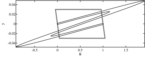
(a) Formation of a horseshoe

$y=0$

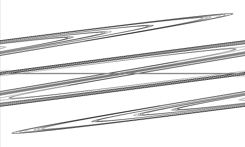
$\theta$

(b) The attractor $\Gamma$

Figure 3: The attractor $\Gamma$ and a horseshoe in it. Panel (a) illustrates the formation of a horseshoe: Shown are a box $R$ (thick gray lines) and its image $\Psi_{\tau}(R)$ (thinner black curves). The vertical boundaries of $R$ are the stable manifolds of the fixed point at $(0,0);$ these are mapped into themselves by $\Psi_{\tau}~{}.$ Panel (b) shows a picture of the attractor $\Gamma.$ The parameters are $\lambda=A=0.1$, $\sigma=2,$ and $\tau=10$ for both plots.

Smale’s horseshoes

Horseshoes are likely present starting from $\sigma$ somewhere between $0.5$ and $1$ for $\tau$ large enough. An example of an easily recognizable horseshoe for $\sigma=2$ and $\tau=10$ is shown in Fig. 3(a). The larger $\sigma$, the easier it is to give examples.

Fig. 3(a) illustrates how proofs of horseshoes or uniformly hyperbolic invariant sets are often done: One first “spots” a horseshoe with one’s eyes, namely one or more boxes that map across themselves in a characteristic way, and then proves that the set of points that remain in these boxes forever has the required splitting into expanding and contracting directions. When $\frac{\sigma}{\lambda}$ is large, $D\Psi_{\tau}$ expands strongly in the $\theta$-direction for most values of $\theta$; contraction is guaranteed since $\det(D\Psi_{\tau})=e^{-\lambda\tau}<1$.

Proposition 2.2 ([29])

Given $\lambda\tau$, $\Psi_{\tau}$ has a horseshoe if $\frac{\sigma}{\lambda}A$ is sufficiently large.

The presence of horseshoes is sometimes equated with dynamical complexity or chaos in the literature, and that is entirely justified insofar as one refers to the existence of chaotic orbits. One must not confuse the existence of these orbits with chaotic behavior starting from “most” or “typical” initial conditions, however: A system can have a horseshoe (which attracts a Lebesgue measure zero set), and have all other points in the phase space tending to a sink. Or, the horseshoe can be part of a “strange attractor”, with $\Lambda_{\max}>0$. The presence of a horseshoe alone does not tell us which of these scenarios will prevail. We will say more about strange attractors versus sinks in Sect. 3.1. Suffice it to observe here that horseshoes clearly exist for most of the parameters in Fig. 2(d)-(f), and $\Lambda_{\max}$ is sometimes positive and sometimes negative.

Sinks from homoclinic tangencies

For larger shear, the attractor can be quite complicated; see Fig. 3(b). Yet in Figs. 2(d), (e), and even (f), sinks can also occur as noted.

The following is purely theoretical, in the sense that we do not know exactly where the sinks are in these specific systems, but it is a general fact in two dimensions that near homoclinic tangencies of dissipative saddle fixed points (“dissipative” means $|\det(Df)|<1$), sinks form easily, meaning one can perturb the map and find one near such a tangency; see [17]. Furthermore, tangencies persist once the stable and unstable manifolds of a horseshoe are shown to meet tangentially somewhere. While no results have been proved for this particular model, the “turns” made by unstable manifolds (see Fig. 3(b)) suggest the abundance of opportunities for such tangencies.

3 A theory of strange attractors

In this section we focus on the case of positive Lyapunov exponents, having discussed negative and zero values of $\Lambda_{\max}$ in Section 2. A combination of geometric and statistical ideas will be used. Since these developments are more recent, we think it may be useful to include more background information: Sect. 3.1 discusses SRB measures for general chaotic systems. Sect. 3.2 surveys some recent work on a class of strange attractors called rank-one attractors. In certain parameter ranges, the attractors $\Gamma$ in our kicked oscillator systems are of this type. In Sect. 3.3, we explain how the general results reviewed in Sects. 3.1 and 3.2 are applied to Eq. (1).

3.1 SRB measures

The setting of this subsection is as follows: Let $M$ be a Riemannian manifold or simply $\mathbb{R}^{n}$. We consider an open set ${U}\subset M$ with compact closure, and let $f$ be a $C^{2}$ embedding of ${U}$ into itself with $\overline{f({U})}\subset{U}$. We will refer to $\Gamma=\cap_{n\geq 0}f^{n}({U})$ as the attractor and ${U}$ as its basin of attraction. Though not a formal assumption, we have in mind here situations that are “chaotic”; in particular, $\Gamma$ is more complicated than an attracting periodic orbit.

We will adopt the viewpoint that observable events are represented by positive Lebesgue measure sets, and are interested in invariant measures that reflect the properties of Lebesgue measure, which we denote by $m$. For chaotic systems, the only invariant measures known to have this property are SRB measures. (The terms Lebesgue and Riemannian measures will be used interchangeably in this article.)

Definition 3.1

An $f$-invariant Borel probability measure $\mu$ is called an SRB measure if

(a) $\Lambda_{\max}>0\ \mu$-a.e., and

(b) the conditional measures of $\mu$ on local unstable manifolds have densities with

respect to the Riemannian measures on these manifolds.

Recall from the Multiplicative Ergodic Theorem [18] that Lyapunov exponents, in particular $\Lambda_{\max}$, are defined $\mu$-a.e., so (a) makes sense; in general, these quantities may vary from point to point. The meaning of (b) can be understood as follows. For an invariant measure to reflect the properties of $m$, it is simplest if it has a density with respect to $m$, but that is generally not possible for attractors: All invariant measures in ${U}$ must live on $\Gamma$, and if $f$ is volume decreasing, which is often the case near an attractor, then $m(\Gamma)=0$. The idea of SRB measures is that if $\mu$ cannot have a density, then the next best thing is for it to have a density in unstable directions, the intuition being that the stretching of phase space in these directions leads to a smoothing of distributions.

The main result on SRB measures is summarized in the next Proposition, followed by a sketch of its proof. The ideas in the proof will explain how SRB measures, which are themselves singular, are related to Lebesgue measure. Recall that for an ergodic measure $\mu$, $\Lambda_{\max}$ is constant $\mu$-a.e. We will denote this number by $\Lambda_{\mu}$.

Proposition 3.1

Let $(f,\mu)$ be an ergodic SRB measure with no zero Lyapunov exponents. Then there is a set ${V}\subset{U}$ with $m(V)>0$ such that the following hold for every $y\in{V}$:

(i) $\Lambda_{\max}(y)=\Lambda_{\mu}$; and

(ii) $\frac{1}{n}\sum_{i=0}^{n-1}\varphi(f^{i}y)\to\int\varphi d\mu\$ for every continuous observable $\varphi:{U}\to{\mathbb{R}}.$

The idea of the proof is as follows: Let $\gamma$ be a piece of local unstable manifold, and let $m_{\gamma}$ be the Riemannian measure on $\gamma$. By property (b) of Definition 3.1, we may assume $m_{\gamma}$-a.e. $x\in\gamma$ is “typical” with respect to $\mu$. In particular, it has properties (i) and (ii) in the Proposition. Let $W^{s}(x)$ be the stable manifold through $x$. Properties (i) and (ii) for $y\in W^{s}(x)$ follow from the corresponding properties for $x$ because $d(f^{n}x,f^{n}y)\to 0$ exponentially as $n\to\infty$. It remains to show that the set of points $y$ that are connected to $\mu$-typical points as above has positive $m$-measure, and that is true by the absolute continuity of the stable foliation [21].

A little bit of history: SRB measures were invented by Sinai, Ruelle and Bowen in the 1970s, when they constructed for every attractor satisfying Smale’s Axiom A [25] a special invariant measure with the properties in Definition 3.1 ([24, 22, 4]). This special invariant measure has a number of other interesting properties; see e.g. [3, 34] for more information. At about the same time, building on Oseledec’s theorem on Lyapunov exponents [18], Pesin [20] and Ruelle [23] extended the uniform theory of hyperbolic systems, also known as Axiom A theory, to an almost-everywhere theory in which positive and negative Lyapunov exponents replace the uniform expansion and contraction in Axiom A. The idea of an SRB measure was brought to this broader setting and studied there by mostly Ledrappier and Young; see e.g. [11].

The existence problem

While the idea and relevant properties of SRB measures were shown to make sense in this larger setting, existence was not guaranteed. Indeed for an attractor outside of the Axiom A category, no matter how chaotic it appears, there is, to this day, no general theory that will tell us whether or not it has an SRB measure.

Here is where the difficulty lies: By definition, an Axiom A attractor has well-separated expanding and contracting directions that are invariant under the dynamics, so that tangent vectors in expanding directions are guaranteed some amount of growth with every iterate. In general, an attractor that appears chaotic to the eye must expand somewhere; this is how instabilities are created. But since volume is decreased, there must also be directions that are compressed. Without further assumptions, for most points $x$ and tangent vectors $v$, $\|Df_{x}^{n}v\|$ will sometimes grow and sometimes shrink as a function of $n$. To prove the existence of an SRB measure, one must show that on balance, $\|Df_{x}^{n}v\|$ grows exponentially for certain coherent families of tangent vectors. The absence of cancellations between expansion and contraction is what sets Axiom A attractors apart from general chaotic attractors.

3.2 Some recent results on rank-one attractors

This subsection reviews some work by Wang and Young [28, 31, 32] on a class of strange attractors. These attractors have a single direction of instability and strong contraction in all complementary directions. Among systems without a priori separation of expanding and contracting directions (or invariant cones), this is the only class to date for which progress has been made on the existence of SRB measures.

The idea is as follows: One embeds the systems of interest in a larger collection, letting $b$ denote an upper bound on their contraction in all but one of the directions (more precisely the second largest singular value of $Df_{x}$). One then lets $b\to 0$ in what is called the singular limit. If this operation results in a family of well defined 1D maps, and if some of these 1D maps carry strong enough expansion, then one can try to conclude that for small but positive $b$, some of the systems have SRB measures. Obviously, this scheme is relevant only for attractors that have a 1D character to begin with. For these attractors, what is exploited here is the fact that 1D objects, namely those in the singular limit, are more tractable than the original $n$-dimensional maps.

Since it is not illuminating to include all technical details in a review such as this one, we refer the reader to [31], Sect. 1, for a formal statement, giving only enough information here to convey the flavor of the main result:

Let $M=I\times D_{n-1}$ where $I$ is either a finite interval or the circle $\mathbb{S}^{1}$ and $D_{n-1}$ is the closed unit disk in ${\mathbb{R}}^{n-1}$, $n\geq 2$. Points in $M$ are denoted by $(x,y)$ where $x\in I$ and $y=(y^{1},\cdots,y^{n-1})\in D_{n-1}$, and $I$ is sometimes identified with $I\times\{(0,\cdots,0)\}$. Given $F:M\to I$, we associate two auxiliary maps:

$$F^{\sharp}:M\to M \quad{\rm where}\quad F^{\sharp}=(F,0,\cdots,0)\ ,$$

$$f:I\to I \quad{\rm where}\quad f=F|_{I\times\{(0,\cdots,0)\}}\ .$$

We need to explain one more terminology: There is a well known class of 1D maps called Misiurewicz maps [16]. Roughly speaking, a map $f$ is in this class if it is $C^{2}$, piecewise monotonic with nondegenerate critical points, and satisfies the following conditions: (i) it is expanding away from $C=\{f^{\prime}=0\}$, and (ii) the forward orbit of every $\hat{x}\in C$ is trapped in an expanding invariant set (bounded away from $C$). Maps in this class are known to have positive Lyapunov exponents Lebesgue-a.e.

Theorem 1 ([31])

Let $F_{a}:M\to I$ be a 1-parameter family of $C^{3}$ maps with the following properties:

(C1) there exists $a^{*}$ such that $f_{a^{*}}$ is a Misiurewicz map;

(C2) $a\mapsto f_{a}$ satisfies a transversality condition at $a=a^{*}$ and $\hat{x}\in C(f_{a^{*}})$;

(C3) for every $\hat{x}\in C(f_{a^{*}})$, there exists $j$ such that $\partial_{y^{j}}F_{a^{*}}(\hat{x},0)\neq 0\$.

Then there exists $b>0$ (depending on $\{F_{a}\}$) such that if $T_{a}:M\to M$ is a family of $C^{3}$ embeddings of $M$ into itself with $\|T_{a}-F_{a}^{\sharp}\|_{C^{3}}<b$, then there is a positive measure set $\Delta$ in $a$-space such that for all $a\in\Delta$, $T_{a}$ admits an SRB measure.

That $\|T_{a}-F_{a}^{\sharp}\|_{C^{3}}$ must be sufficiently small is the rank one condition discussed above, and (C1) is where we require the singular limit maps to have sufficient expansion. Notice that (C1)–(C3) all pertain to behavior at or near $a=a^{*}$. The set $\Delta$ will also be in the vicinity of this parameter. (C2) guarantees that one can bring about changes effectively by tuning the parameter $a$, and (C3) is a nondegeneracy condition at the critical points.

Remark. The existence of SRB measures is asserted for a positive measure set of parameters, and not for, say, an entire interval of $a$. This is a reflection of reality rather than a weakness of the result: there are parameters $a$ arbitrarily near $\Delta$ for which $T_{a}$ has sinks. In a situation such as this one where chaotic and non-chaotic regimes coexist in close proximity of one another, it is impossible to say for certain if any given map has an SRB measure. One can conclude, at best, that nearby maps have SRB measures “with positive probability”.

Theorem 1 was preceded by the corresponding result for the Hénon family

$$T_{a,b}:(x,y)\mapsto(1-ax^{2}+y,bx)\ .$$ (4)

The existence of SRB measures for parameters near $a^{*}=2$ and $b\ll 1$ was proved in [2] building on results from [1]. This is the first time the existence of SRB measures was proved for genuinely nonuniformly hyperbolic attractors. Even though [1] is exclusively about Eq. (4), the techniques developed there were instrumental in the proof of Theorem 1.

Returning to the setting of Theorem 1, let us call $a\in\Delta$ a “good parameter” and $T=T_{a}$ a “good map”. The following two properties of these maps are directly relevant to us. They were proved under the following additional assumption on $M$:

$$|\det(DT_{a})|\sim b^{n-1}\ . \star$$ ()

• Lebesgue-a.e. $z\in M$ is contained in $W^{s}(\xi)$ where $\xi$ is typical with respect to an ergodic SRB measure (in general, there may be more than one such measure). It follows that $\Lambda_{\max}(z)>0$ for Lebesgue-a.e. $z\in M$.

• Another condition on $f_{a^{*}}$ (Lyapunov exponent $>\log 2$ and $f_{a^{*}}^{N}$ mapping every interval of monotonicity to all of $I$ for some $N$) implies the uniqueness of SRB measure. This in turn implies $\Lambda_{\max}$ is constant a.e. in $M$.

These and a number of other results for “good maps” were proved in [32]. We mention one that is not used here but sheds light on the statistical properties of these attractors: For an SRB measure $\mu$ for which $(T,\mu)$ is mixing, the system has exponential decay of correlations for Lipschitz observables, i.e., there exists $\tau\in(0,1)$ such that for all Lipschitz $\varphi,\psi$, there exists $C=C(\varphi,\psi)$ such that for all $n\geq 1$,

$$\left|\int(\varphi\circ T^{n})\psi~{}d\mu-\int\varphi~{}d\mu\int\psi~{}d\mu\right|\leq C\tau^{n}\ .$$

3.3 Application to kicked oscillators

We now return to the model introduced in Sect. 1.1 and explain how this system can be fitted into the framework of the last subsection. (See [29] for details.) We fix $\sigma,\lambda,A$, and allow $\tau$ to vary. Writing $\tau=k+a$ where $k=[\tau]$, the integer part of $\tau$, we let $T_{k,a}=\Psi_{\tau}$. For each fixed $k\in\mathbb{Z}^{+}$, we view $\{T_{a}=T_{k,a},a\in[0,1)\}$ as the family of interest, and discuss if and when the conditions of Theorem 1 will hold for this family.

Here, the singular limit maps $F_{a}$ are well defined. In fact, they are the first components of $\lim_{k\to\infty}T_{k,a}$, i.e.,

$$F_{a}(\theta,y)=\theta+a+\frac{\sigma}{\lambda}\cdot(y+A\sin(2\pi\theta))\ ,$$

and the restriction of $F_{a}$ to ${\mathbb{S}}^{1}$ is

$$f_{a}:{\mathbb{S}}^{1}\to{\mathbb{S}}^{1},\qquad f_{a}(\theta)=\theta+a+\frac{\sigma}{\lambda}A\sin(2\pi\theta),\qquad a\in[0,1)\ .$$ (5)

Notice immediately that the range of applicability of Theorem 1 is limited to $\lambda\tau$ relatively large. This is because $\|T_{k,a}-F_{a}^{\sharp}\|_{C^{3}}={\cal O}(b)$ where $b=e^{-\lambda k}$ is required to be very small. For a given unforced system, where the amount of damping $\lambda$ is fixed, this means the kicks must be applied sufficiently far apart in time.

We comment on (C1), which along with the rank one condition above are the core assumptions for this theorem. For our purposes let us assume $f_{a}$ satisfies the Misiurewicz condition if some iterate of $f_{a}$ sends its two critical points $c_{1}$ and $c_{2}$ into an unstable periodic orbit or an expanding invariant Cantor set. First, such Cantor sets are readily available for medium size values of $\frac{\sigma}{\lambda}$ such as $\frac{\sigma}{\lambda}\geq 1$, and unstable periodic orbits start to exist for somewhat smaller values of $\frac{\sigma}{\lambda}$. Suppose for some parameter value $a$ that the forward orbit of $c_{1}$ is contained in an expanding invariant set $K$. As we vary $a$, both the orbit of $c_{1}$ and $K$ will move with $a$. Condition (C2), assuming it holds, implies that for all large enough $k\in{\mathbb{Z}}^{+}$, $f^{k}_{a}(c_{1})$ moves faster, i.e., the path traced out by $a\mapsto f^{k}_{a}(c_{1}(a))$ cuts across $K$ as though the latter was stationary. When $K$ is a Cantor set, this guarantees that $f^{k}_{a}(c_{1})\in K$ for an uncountable number of $a$’s. By symmetry, when that happens to $f_{a}(c_{1})$, the same is automatically true for $f_{a}(c_{2})$. The larger $\frac{\sigma}{\lambda}$, the denser these Cantor sets are in $\mathbb{S}^{1}$, and the denser the set of parameters $a$ that can be taken to be $a^{*}$ in (C1).

The checking of (C2), (C3), and ($\star$) are straightforward. Conditions for the uniqueness of SRB measures require that $\frac{\sigma}{\lambda}$ be a little larger.

To summarize, the results in the last subsection imply that for $\frac{\sigma}{\lambda}\geq 1$ (or even smaller), for all large enough $k$, there exist positive measure sets $\Delta_{k}$ such that for $a\in\Delta_{k}$ and $\tau=k+a$, $\Psi_{\tau}$ is a “good map” in the sense of the last subsection. In particular, $\Psi_{\tau}$ has an SRB measure. We conclude also that $\Lambda_{\max}(z)$ is well defined and $>0$ for Lebesgue-a.e. $z\in U$. To ensure that $\Lambda_{\max}(z)=$ constant a.e. (so there are no open squares in Fig. 2) one needs to take $\frac{\sigma}{\lambda}$ a little larger. It is in fact not hard to see that $\Delta_{k}\approx\Delta_{k^{\prime}}$ for $k\neq k^{\prime}$ when both are sufficiently large, so that in this parameter range, the set of $\tau$ for which the properties above are enjoyed by $\Psi_{\tau}$ is roughly periodic with period $1$.

Remarks on analytic results for chaotic systems

Theorem 1 is a perturbative result. As is generally the case with perturbative proofs, the sizes of the perturbations (such as $b$) are hard to control. Consequently, applicability of Theorem 1 is limited to regimes with very strong contraction. The results reported in Sect. 3.2, however, are the only rigorous results available at the present time. Techniques for analyzing maps in parameter ranges such as those in Fig. 2 are lacking and currently quite far out of reach.

The situation here is a reflection of the general state of affairs: Due to the cancellations discussed at the end of Sect. 3.1, rigorous results for the large-time behavior of chaotic dynamical systems tend to be challenging.

When results such as Theorem 1 are available, however, they – and the ideas behind them – often shed light on situations that are technically beyond their range of applicability. Our example here is a good illustration of that: Fig. 2(d)-(f) show that as $\frac{\sigma}{\lambda}A$ increases, positive Lyapunov exponents become more abundant among the parameters tested, interspersed with occasional sinks. This is in agreement with the dynamical picture suggested by Theorem 1 even though with $\lambda\tau\in[0.5,1.5]$, the contraction can hardly be considered strong.

4 Generalizations

In Sections 1, 2, and 3.3, we have focused on a concrete model. We now generalize this example in two different ways:

• the unforced equation in Eq. (1) is replaced by an arbitrary limit cycle;

• the specific kick in Eq. (1) is replaced by an arbitrary kick.

More precisely, we consider a smooth flow $\Phi_{t}$ on a finite dimensional Riemannian manifold (which can be ${\mathbb{R}}^{n}$), and let $\gamma$ be a hyperbolic limit cycle, i.e., $\gamma$ is a periodic orbit of period $p$, and for any $x\in\gamma$, all eigenvalues for $D\Phi_{p}(x)$ are $<1$ aside from that in the flow direction. The basin of attraction of $\gamma$ is the set ${\cal B}:=\{x\in M:\Phi_{t}(x)\to\gamma$ as $t\to\infty\}$. We continue to consider forcing in the form of kicks, and assume for simplicity that the kicks are defined by a smooth embedding $\kappa:M\to M$ (as would be the case if, for example, $\kappa$ represents the result of a forcing defined by $\dot{z}=G(z,t)$ where the vector field $G(z,t)$ is nonzero, or “on,” for only a short time). As before, the kicks are applied periodically at times $0,\tau,2\tau,3\tau,\dots$, and the time evolution of the kicked system is given by $\Psi_{\tau}=\Phi_{\tau}\circ\kappa$.

A new issue that arises in this generality is that one may not be able to isolate the phenomenon, that is to say, the kicking may cause the limit cycle to interact with dynamical structures nearby. Our discussion below is limited to the case where this does not happen, i.e., we assume there is an open set $U$ with $\gamma\subset U\subset{\cal B}$ such that $\kappa(U)\subset{\cal B}$ and $\Phi_{\tau}(\kappa(U))\subset U$, and define $\Gamma=\cap_{n}\Psi_{\tau}^{n}({U})$ to be the attractor of the kicked system as before.

We further limit the scope of our discussion in the following two ways: (i) Kicks that are too weak will not be considered; such kicks produce invariant curves and sinks for the same reasons given in Sect. 2.1, and there is no need to discuss them further. (ii) We consider only regimes that exhibit a substantial contraction during the relaxation period, brought about by long enough kick intervals that permit the “shear” to act. As we will see, this is a more tractable situation. Rigorous results can be formulated – and we will indicate what is involved – but will focus primarily on ideas. Precise formulations of results in this generality (see [30]) are unfortunately not as illuminating as the phenomena behind them.

The geometry of folding: kicks and the strong stable foliation

As we will show, key to understanding the effects of kicks is the geometric relation between the kick and the strong stable foliation associated with the limit cycle of the unforced system. For $x\in\gamma$, we define the strong stable manifold of $\Phi_{t}$ at $x$, denoted $W^{ss}(x)=W^{ss}_{\Phi_{t}}(x)$, to be the set $W^{ss}(x)=\{y\in M:d(\Phi_{t}(y),\Phi_{t}(x))\to 0$ as $t\to\infty\}$; the distance between $\Phi_{t}(x)$ and $\Phi_{t}(y)$ in fact decreases exponentially; see e.g. [10]. (This stable manifold is for the flow $\Phi_{t}$, not to be confused with that for the kicked map $\Psi_{\tau}$ in Prop. 2.1.) Some basic properties of these manifolds are: (i) $W^{ss}(x)$ is a codimension one submanifold transversal to $\gamma$ and meets $\gamma$ at exactly one point, namely $x$; (ii) $\Phi_{t}(W^{ss}(x))=W^{ss}(\Phi_{t}(x))$, and in particular, if the period of $\gamma$ is $p$, then $\Phi_{p}(W^{ss}(x))=W^{ss}(x)$; and (iii) the collection $\{W^{ss}(x),x\in\gamma\}$ foliates the basin of attraction of $\gamma$. An example of a $W^{ss}$-foliation for a limit cycle is shown in Fig. 4.

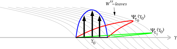
Figure 4: Geometry of folding in relation to the $W^{ss}$-foliation. Images of $\Psi_{\tau_{1}}(\gamma_{0})$ and $\Psi_{\tau_{2}}(\gamma_{0})$ for $\tau_{1}<\tau_{2}$, both multiples of the period of the limit cycle $\gamma$, are shown.

Fig. 4 shows the image of a segment $\gamma_{0}$ of $\gamma$ under $\Psi_{\tau}$. For illustration purposes, we assume $\gamma_{0}$ is kicked upward with its end points held fixed, and assume $\tau=np$ for some $n\in{\mathbb{Z}}^{+}$ where $p$ is the period of the cycle. Since $\Phi_{np}$ leaves each $W^{ss}$-manifold invariant, we may imagine that during relaxation, the flow “slides” each point of the curve $\kappa(\gamma_{0})$ back toward $\gamma$ along $W^{ss}$-leaves; the larger $n$ is, i.e., the more times it laps around, the farther down the point slides. In the situation depicted, the folding is quite evident. If $\tau$ is not an integer multiple of $p$, then $\Phi_{\tau}$ carries each $W^{ss}$-manifold to another $W^{ss}$-manifold. Writing $\tau=np+a$ where $a\in[0,p)$, we can think of the action of $\Phi_{\tau}$ as first sliding along the $W^{ss}$-manifold by an amount corresponding to $\Phi_{np}$ and then flowing forward for time $a$.

The picture in Fig. 4 gives insight into what types of kicks are likely to produce chaos. The following observations are intended to be informal but intuitively clear:

• Kicks directed along $W^{ss}$-leaves or in directions roughly parallel to $W^{ss}$-leaves are not effective in producing chaos, nor are kicks that essentially carry one $W^{ss}$-leaf to another in an order-preserving fashion. For such kicks, $\Psi_{\tau}$ essentially permutes $W^{ss}$-leaves, and $\kappa$ has to overcome the contraction within individual leaves to create chaotic behavior. (This cannot happen in 2D.)

• The stretch-and-fold mechanism for producing chaos remains valid: the more $\Psi_{\tau}(\gamma)$ is folded, the more chaotic the system is likely to be, i.e., the intuition is as in Fig. 1. What is different here is that unlike our earlier example, where the propensity for shear-induced chaos is determined entirely by parameters in the unforced equation, namely $\sigma$ and $\lambda$, we see in this more general setting that it matters how the kick is applied. It is the geometry of the action of $\kappa$ on the limit cycle $\gamma$ in relation to the strong stable foliation $W^{ss}$ that determines the stability or chaos of the kicked system.

• The case of stronger contraction is more tractable mathematically for the following reason: When the contraction in $\Psi_{\tau}$ is weak, as with $\tau=\tau_{1}$ in Fig. 4, one has to deal with the cumulative effects of multiple kicks, which are difficult to treat. When the image $\Psi_{\tau}(\gamma_{0})$ is pressed more strongly against $\gamma$, as in the case of $\tau=\tau_{2}>\tau_{1}$, cumulative effects of consecutive kicks are lessened.

We illustrate some of the ideas above in the examples below.

Linear shear-flow examples

The 2D system in Eq. (1): The ideas in this section can be seen as an abstraction of those discussed earlier. To understand that, we compute the $W^{ss}$-leaves of the unforced equation in Eq. (1), and find them to be straight lines having slopes $-\frac{\lambda}{\sigma}$. We concluded earlier that given $A$, the larger $\frac{\sigma}{\lambda}$, i.e., the smaller the angle between the $W^{ss}$-leaves and $\gamma$, the more chaotic the system is likely to be. Item (ii) above corroborates this conclusion: Given that we kick perpendicularly to the limit cycle (as is done in Eq. (1)), and points in $\gamma$ are kicked to a given height, the more “horizontal” the $W^{ss}$-leaves, the farther the points in $\kappa(\gamma)$ will slide when we bring them back to $\gamma$. In other words, the $\frac{\sigma}{\lambda}$ part of the ratio from earlier is encoded into the geometry of the $W^{ss}$-foliation — provided that we kick perpendicularly to the cycle.

Generalization to $n$ dimensions: The $n$-dimensional analog of Eq. (1) with a more general forcing is

$$\begin{array}[]{ccl}\dot{\theta}&=&1+\sigma\cdot{\bf y}\ ,\\[4.30554pt] \dot{\bf y}&=&-\Lambda{\bf y}+AH(\theta){\bf v}(\theta)\cdot\sum_{n=-\infty}^{\infty}\delta(t-n\tau)\ ,\\ \end{array}$$ (6)

where $\theta\in{\mathbb{S}}^{1}$, ${\bf y}\in{\mathbb{R}}^{n-1}$, $\sigma\in\mathbb{R}^{n-1}$ is nonzero, and $\Lambda$ is an $(n-1)\times(n-1)$ matrix all of whose eigenvalues have strictly positive real parts. For simplicity, we assume the kicks are perpendicular to the limit cycle $\{{\bf y}=0\}$, and to facilitate the discussion, we have separated the following aspects of the kick function: its amplitude is $A$, variation in $\theta$ is $H(\theta)$, and the direction of the kick is ${\bf v}(\theta)\in{\mathbb{S}}^{n-2}$. As a further simplification, let us assume ${\bf v}(\theta)\equiv{\bf v}\in{\mathbb{R}}^{n-1}$, i.e., it is a fixed vector.

A computation shows that the $W^{ss}$-manifolds of the unforced equation are given by

$$W^{ss}(\theta_{0},{\bf 0})=\{(\theta,{\bf y}):\theta=\theta_{0}-\sigma^{T}{\bf\Lambda}^{-1}{\bf y}\},$$

i.e., they are hyperplanes orthogonal to the covector $(1,\sigma^{T}{\bf\Lambda}^{-1})$ . As noted in item (i) above, kick components orthogonal to $(1,\sigma^{T}{\bf\Lambda}^{-1})$ are “dissipated” and do not have much effect. If $H\equiv$ constant, then $\Psi_{\tau}$ simply permutes the $W^{ss}$-planes and again no chaotic behavior will ensue. To produce horseshoes and strange attractors, a sufficient amount of variation in $\theta$ for $\Psi_{\tau}(\gamma)$ is needed as noted in item (ii) above; that variation must come from $H$. An analysis similar to that in Eq. (2), Sect. 1.2, tells us that for large $\tau$, the amount by which the kick is magnified in the $\theta$-direction is $\approx A~{}H(\theta)~{}\sigma^{T}{\bf\Lambda}^{-1}{\bf v}$ . We remark that the variation in $H$ is far more important than its mean value, which need not be $0$.

Finally, given $H\not\equiv$ constant, to maximize the variation of $\Psi_{\tau}(\gamma)$ in $\theta$ for large $\tau$, the discussion above suggests kicking in a direction ${\bf v}$ that maximizes $\sigma^{T}{\bf\Lambda}^{-1}{\bf v}$. Under the conditions above, this direction is unique and is given by ${\bf v}=\pm({\bf\Lambda^{T}})^{-1}\sigma/|({\bf\Lambda^{T}})^{-1}\sigma|$. Notice that this need not be the direction with the least damping or the direction with maximal shear, but one that optimizes the combined effect of both.

On analytic proofs

When $\Psi_{\tau}$ contracts strongly enough, the system falls into the rank one category as defined in Sect. 3.2, independently of the dimension of the phase space. This comes from the fact that $\Phi_{t}$ carries all points back to $\gamma$, which is a one-dimensional object.

If the folding (as described in item (ii) above) is significant enough for the amount of contraction present, then horseshoes can be shown to exist. Proving the existence of horseshoes with one unstable direction is generally not very difficult, and not a great deal of contraction is needed.

To prove the existence of strange attractors or SRB measures, the results in Sect. 3.2 are as applicable here as in our 2D linear example. It is proved in [30] that the periodic kicking of arbitrary limit cycles fits the general framework of Theorem 1, in the sense that as the time between kicks tends to infinity, singular limit maps are well defined. They are given by $f_{a}:\gamma\to\gamma$, $a\in[0,p)$, where

$$f_{a}(x)\ :=\ \lim_{n\to\infty}\Phi_{np+a}(\kappa(x))\qquad\mbox{ for all }x\in\gamma\ .$$

From our earlier discussion of sliding along $W^{ss}$-leaves, it is not hard to see that $f_{a}(x)$ is, in fact, the unique point $y\in\gamma$ such that $\kappa(x)\in W^{ss}(y)$. Whether (C1)–(C3) hold depends on the system in question and hinges mostly on (C1), which usually holds when the variation is large enough. As always, these conditions need to be verified from example to example.

Related Results and Outlook

We have reviewed a set of results on the periodic kicking of limit cycles. The main message is that the effect of the kick can be magnified by the underlying shear in the unforced system to create an unexpected amount of dynamical complexity. It is an example of a phenomenon known as shear-induced chaos.

A similar geometric mechanism is used to prove the existence of strange attractors in (a) certain examples of slow-fast systems [8]; (b) periodic kicking of systems undergoing supercritical Hopf bifurcations (see [30] for details, and [15] for results applicable to evolutionary PDEs); and (c) periodic forcing of near-homoclinic loops [27]. See also [19]. All of these results pertain to strong-contraction regimes; proofs are perturbative and rely on the theory of rank one attractors reviewed in Sect. 3.2.

A welcome extension of the results reviewed here is to remove the strong-contraction assumption for strange attractors, but this is likely to be challenging: one has to either develop non-perturbative techniques or go about the problem in a less direct way.

Random forcing is a future direction we believe to be both interesting and promising. Numerical studies of Poisson and white-noise forcing have been carried out [14]. Phenomena similar to those in Sect. 1 are observed when the kick term in Eq. (1) is replaced by a term of the form $A\sin(2\pi\theta)~{}dB_{t}$ where $B_{t}$ is standard Brownian motion, i.e., the setup is a stochastic differential equation. With stochastic forcing, phase space geometry is messier, but $\Lambda_{\max}$ depends continuously on parameters. The absence of wild fluctuations between positive and negative values of $\Lambda_{\max}$ (corresponding respectively to strange attractors and sinks in the periodic case) gives hope to the idea that the analysis for stochastic forcing may be more tractable than that for periodically forced systems.

References

- [1] M. Benedicks and L. Carleson, “The dynamics of the Hénon map,” Ann. Math. 133 (1991) pp. 73–169
- [2] M. Benedicks and L.-S. Young, “Sinai-Bowen-Ruelle measures for certain Henon maps,” Invent. Math. 112 (1993) pp. 541–576
- [3] R. Bowen, Equilibrium States and the Ergodic Theory of Anosov Diffeomorphisms, Lecture Notes in Mathematics 470, Springer-Verlag, New York (1975)
- [4] R. Bowen and D. Ruelle, “The ergodic theory of Axiom A flows,” Invent. Math. 29 (1975) pp. 181–202
- [5] M. L. Cartwright and J. E. Littlewood, “On nonlinear differential equations of the second order,” J. London Math. Soc. 20 (1945) pp. 180–189
- [6] R. FitzHugh, “Impulses and physiological states in theoretical models of nerve membrane,” Biophys. J. 1 (1961) pp. 445–466
- [7] J. Guckenheimer and P. Holmes, Nonlinear Oscillations, Dynamical Systems, and Bifurcations of Vector Fields, Springer-Verlag (1983)
- [8] J. Guckenheimer, M. Wechselberger, and L.-S. Young, “Chaotic attractors of relaxation oscillators,” Nonlinearity 19 (2006) pp. 701–720
- [9] R. Haiduc, “Horseshoes in the forced van der Pol system,” Nonlinearity 22 (2009) pp. 213–237
- [10] M. W. Hirsch, C. C. Pugh, and M. Shub. Invariant Manifolds. Lecture Notes in Mathematics 583, Springer-Verlag, New York (1977)
- [11] F. Ledrappier and L.-S. Young, “The metric entropy of diffeomorphisms,” Ann. Math. 122 (1985) pp. 509–574
- [12] M. Levi, “Qualitative analysis of periodically forced relaxation oscillations,” Mem. AMS 214 (1981) pp. 1–147
- [13] N. Levinson, “A second order differential equation with singular solutions,” Ann. Math. 50 No. 1 (1949) pp. 127–153
- [14] K. K. Lin and L.-S. Young, “Shear-induced chaos,” Nonlinearity 21 (2008) pp. 899–922
- [15] K. Lu, Q. Wang, and L.-S. Young. “Strange attractors for periodically forced parabolic equations,” preprint
- [16] M. Misiurewciz, “Absolutely continuous measures for certain maps of an interval,” Publ. Math. l’IHÉS 53 (1981) pp. 17–51
- [17] S. Newhouse, Lectures on Dynamical Systems, Progress in Math. 8, Birkhäuser (1980) pp. 1–114
- [18] V. I. Oseledec, “A multiplicative ergodic theorem: Liapunov characteristic numbers for dynamical systems,” Trans. Moscow Math. Soc. 19 (1968) pp. 197–231
- [19] W. Ott and M. Stenlund, “From limit cycles to strange attractors,” Commun. Math. Phys. 296 (2010) pp. 215–249
- [20] Ja. B. Pesin, “Characteristic Lyapunov exponents and smooth ergodic theory,” Russ. Math. Surv. 32.4 (1977) pp. 55–114
- [21] C. Pugh and M. Shub, “Ergodic attractors,” Trans. AMS 312 (1989) pp. 1–54
- [22] D. Ruelle, “A measure associated with Axiom A attractors,” Amer. J. Math. 98 (1976) pp. 619–654
- [23] D. Ruelle, “Ergodic theory of differentiable dynamical systems,” Publ. Math., Inst. Hautes Étud. Sci. 50 (1979) pp. 27–58
- [24] Ya. G. Sinai, “Gibbs measure in ergodic theory,” Russian Math. Surveys 27 (1972) pp. 21–69
- [25] S. Smale, “Differentiable dynamical systems,” Bull. Amer. Math. Soc. 73 (1967) pp. 747-–817
- [26] B. van der Pol and J. van der Mark, “Frequency demultiplication,”Nature 120 (1927) pp. 363–364
- [27] Q. Wang and W. Ott, “Dissipative homoclinic loops and rank one chaos,” preprint
- [28] Q. Wang and L.-S. Young, “Strange attractors with one direction of instability,” Comm. Math. Phys. 218 (2001) pp. 1–97
- [29] Q. Wang and L.-S. Young, “From invariant curves to strange attractors,” Comm. Math. Phys. 225 (2002) pp. 275–304
- [30] Q. Wang and L.-S. Young, “Strange attractors in periodically-kicked limit cycles and Hopf bifurcations,” Comm. Math. Phys. 240 (2003) pp. 509–529
- [31] Q. Wang and L.-S. Young, “Toward a theory of rank one attractors,” Ann. Math. 167 (2008) pp. 349–480
- [32] Q. Wang and L.-S. Young, “Dynamical profile of a class of rank one attractors,” preprint
- [33] A. Winfree, The Geometry of Biological Time, Second Edition, Springer-Verlag (2000)
- [34] L.-S. Young, “What are SRB measures, and which dynamical systems have them?” J. Stat. Phys. 108 (2002) pp. 733–754
- [35] G. Zaslavsky, “The simplest case of a strange attractor,” Physics Letters 69A (1978) pp. 145–147