A bright radio HH object with large proper motions in the massive star-forming region W75N

Abstract

We analyze radio continuum and line observations from the archives of the Very Large Array, as well as X-ray observations from the Chandra archive of the region of massive star formation W75N. Five radio continuum sources are detected: VLA 1, VLA 2, VLA 3, Bc, and VLA 4. VLA 3 appears to be a radio jet; we detect J=1-0, v=0 SiO emission towards it, probably tracing the inner parts of a molecular outflow. The radio continuum source Bc, previously believed to be tracing an independent star, is found to exhibit important changes in total flux density, morphology, and position. These results suggest that source Bc is actually a radio Herbig-Haro object, one of the brightest known, powered by the VLA 3 jet source. VLA 4 is a new radio continuum component, located a few arcsec to the south of the group of previously known radio sources. Strong and broad (1,1) and (2,2) ammonia emission is detected from the region containing the radio sources VLA 1, VLA 2, and VLA 3. Finally, the 2-10 keV emission seen in the Chandra/ACIS image shows two regions that could be the termination shocks of the outflows from the multiple sources observed in W75N.

1 Introduction

The compact, thermal (i. e. free-free) radio sources found at centimeter wavelengths in regions of star formation can have different natures. Some of them are ultracompact or hypercompact HII regions, photoionized by an embedded hot luminous star. Other sources are clumps of gas or even circumstellar disks that are being externally ionized by a nearby star, such as the Orion proplyds (e. g. O’Dell & Wong 1996; Zapata et al. 2004) and the bright-rimmed clouds (e.g. Carrasco-Gonzalez et al. 2006). An additional class of sources is formed by the thermal jets, collimated outflows that emanate from young stars and whose ionization is most probably maintained by the interaction of the moving gas with the surrounding medium (Eisloffel et al. 2000). Finally, there are also some examples of “radio Herbig-Haro” objects, obscured knots of gas that are being collisionally ionized by the shock produced by a collimated outflow (e. g. Curiel et al. 1993). There are also compact non-thermal sources, of which the most common are the young low-mass stars with active magnetospheres that produce gyrosynchrotron emission (e.g. Feigelson & Montmerle 1999). There are also emission regions where fast shocks may produce synchrotron emission (e.g. Henriksen et al. 1991; Garay et al. 1996).

To advance in the understanding of the nature of these compact radio sources it is necessary to have good quality data that allows the observer to establish the angular size, the morphology, the spectral index, the time variability, the polarization, and the presence of proper motions in them. Only a handful of the known star-forming regions have been studied carefully enough to clearly establish the nature of its compact radio sources.

The massive star-forming region W75N is part of the Cygnus X complex of dense molecular clouds. Its distance is estimated to be 2 kpc (Fischer et al. 1985). Haschick et al. (1981) detected at 6 cm a source that was interpreted as an ultracompact HII (UC HII) region named W75N(B), that later was resolved into three small diameter radio continuum sources: Ba, Bb and Bc in the high angular resolution ($0\hbox to0.0pt{.\hss}{{}^{\prime\prime}}5$) observations of Hunter et al. (1994). Two of these sources, Ba and Bb, were also detected at 1.3 cm (with a $0\hbox to0.0pt{.\hss}{{}^{\prime\prime}}1$ resolution) by Torrelles et al. (1997) (who named them as VLA 1 and VLA 3) along with another fainter and more compact source, located in between VLA 1 and VLA 3, and named as VLA 2. These compact sources were believed to be UC HII regions in an early phase, based on the presence of H₂O and/or OH masers (Baart et al. 1986, Hunter et al. 1994, Torrelles et al. 1997) in its close vicinity.

At radio wavelengths, VLA 1 has a structure elongated at a PA of $\sim 43^{\circ}$ (Torrelles et al. 1997), approximately in the direction of the observed high-velocity three pc-scale bipolar outflow (Hunter et al. 1994; Shepherd et al. 2003). However, Shepherd (2001) had pointed that VLA 1 does not appear to contribute significantly to the energetics of the large-scale outflow. VLA 2 shows a symmetric roundish shape. A detailed Very Long Baseline Interferometry (VLBI) study of the water maser cluster morphology and kinematics in the vicinity of these two radio sources by Torrelles et al. (2003) showed remarkably different outflow ejection geometries among them (VLA 1 has a collimated, jetlike outflow, while VLA 2 has a shell outflow expanding in multiple directions). This is a surprising result given that both objects are separated by only 1400 AU and share the same environment. VLA 3 was found to have deconvolved dimensions of $0\hbox to0.0pt{.\hss}{{}^{\prime\prime}}09\times 0\hbox to0.0pt{.\hss}{{}^{\prime\prime}}04$ $(PA=152^{\circ})$ at 1.3 cm by Torrelles et al. (1997). This source is also detected at mid-infrared wavelengths, with a bolometric luminosity of   750 L_⊙ (Persi, Tapia, & Smith 2006). The physical parameters of the ionized gas in VLA 1, VLA 2, VLA 3, and Bc, as well as the more evolved W75N(A) are all consistent with each being powered by a ZAMS star of spectral type between B0 and B2 (Shepherd et al. 2004). The present evidence is consistent with an independent exciting source of this spectral type for each radio continuum component, but the results presented in this paper suggest a likely alternative interpretation.

In this paper we analyze Very Large Array (VLA) and Chandra archive data of the region, mostly searching for variability and proper motions that could help in a better understanding of the radio sources.

2 Observations and Results

The parameters of the VLA archive observations used in this study are summarized in Table 1. All the data were calibrated following the standard VLA procedures. The flux calibrators and the name and bootstrapped flux density of the phase calibrators used in each observation are given in Table 1. In the following sections we describe in more detail the radio and X-ray observations.

2.1 Radio Continuum Emission

In Figure 1 we show the continuum images of the central region of W75N at 3.6 cm (2006.38) and 2 cm (2001.31). As can be seen in this figure, to the south of the previously known components (VLA 1, VLA 2, VLA 3 and Bc), we detected a new radio source, VLA 4. This source was not detected in the other continuum images discussed here (see below), most probably because they are noiser than the 2006 image at 3.6 cm. In Table 2 we show the positions of the five sources (from the 3.6 cm 2006 data) with their flux densities at both wavelengths (3.6 and 2 cm) and their spectral indices in this wavelength range. We note that since some of the sources are time-variable (see below), these spectral indices are not very reliable.

Three of the sources (VLA 1, Bc, and VLA 4) have flat spectral indices within the error, a result consistent with optically thin free-free emission. Source VLA 3 has a spectral index of 0.6$\pm$0.1, consistent with the value expected for a thermal jet. The source with the steepest spectral index is VLA 2, that with a value of 2.2$\pm$0.3 suggests optically thick free-free emission.

In Figure 2 we compare the three 3.6 cm images made from data taken in 1992, 1998, and 2006. Since these observations were not made with the same phase calibrator (see Table 1), we aligned them by assuming that the position of VLA 3 was the same at all three epochs and using the 2006 position for all of them. This alignment involved small position shifts of $\leq 0\hbox to0.0pt{.\hss}{{}^{\prime\prime}}1$. In particular, the shift of the 1998 image to align it with the 2006 image was of only $\Delta\alpha=+0\hbox to0.0pt{.\hss}^{s}007;\Delta\delta=-0\hbox to0.0pt{.\hss}{{}^{\prime\prime}}03$. Of the sources in the region, only source Bc shows important changes in position. Its average proper motion, $0\hbox to0.0pt{.\hss}{{}^{\prime\prime}}3\pm 0\hbox to0.0pt{.\hss}{{}^{\prime\prime}}1$ toward the south, over a time of 13.48 years at a distance of 2 kpc, implies an average velocity in the plane of the sky of 220$\pm$70 km s^-1. However, as can be seen in Figure 2, most of the displacement took place between the last two epochs, so the velocity between these two last epochs is possibly larger.

In addition to the proper motions, there is a dramatic change in flux density and morphology of source Bc at 3.6 cm. In 1992 it was a weak compact source (with a flux density of 0.9$\pm$0.2 mJy), becoming brighter (2.7$\pm$0.5 mJy) and elongated in 1998 (see Figure 2). The position does not seem to change significantly between these two epochs. Finally, in 2006 the source remained bright (3.3$\pm$0.2 mJy) and appears as broken in two components. Furthermore, it has clearly moved to the south.

2.2 Molecular Line Emission

2.2.1 SiO emission

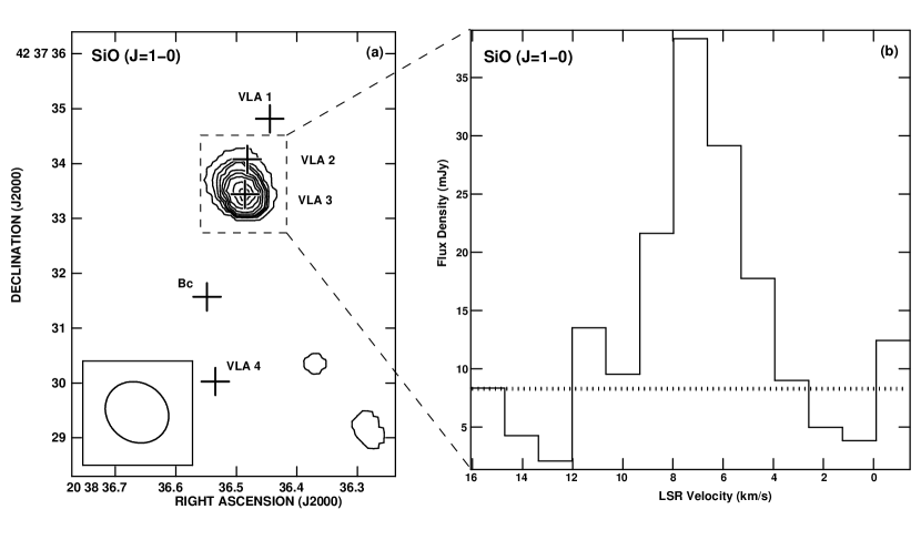
Figure 3: a) VLA contour image of the moment 0 of the J= 1–0; v = 0 SiO emission from the W75N region. Contours are 20, 40, 50, 60, 80, 100, 120, 140, and 160 mJy beam^-1 km s^-1. The beam ($1\hbox to0.0pt{.\hss}{{}^{\prime\prime}}21\times 1\hbox to0.0pt{.\hss}{{}^{\prime\prime}}06$; PA = $52^{\circ}$) is shown in the bottom left corner of the image. The crosses mark the positions of the radio continuum sources. The dashed rectangle indicates the solid angle over which the spectrum of the right panel of this figure was obtained. b) Spectrum of the SiO emission from the box indicated in the left panel. The dotted horizontal line indicates the expected 7-mm continuum contribution, as estimated from the results of Shepherd et al. (2004).

Using VLA archive data, we obtained the image for the J = 1–0; v = 0 emission of the SiO molecule (43.423858 GHz) in the W75N region shown in the left panel of Figure 3. The spectral line observations were made with one IF and a total number of 63 channels, for a velocity resolution of 1.2 km s^-1 and a velocity coverage of $\sim$80 km s^-1. Since these observations did not include an ad hoc bandpass calibrator, we were forced to use as bandpass calibrators the flux (1331+305) and phase (2012+464) calibrators. The image is made from the velocity-integrated (moment 0) emission. The SiO emission is compact and centered on VLA 3, although part of the emission could be coming from VLA 2. The SiO spectrum is shown in the right panel of Figure 3. The observed transition is known to be a tracer of outflows (e.g. Choi 2005). We propose that the SiO emission could be tracing the inner parts of an outflow associated with VLA 3, although observations with much better angular resolution, sensitivity and velocity coverage are needed to test this hypothesis.

2.2.2 NH₃ emission

Also using VLA archive data, we obtained images for the (1,1) and (2,2) inversion transitions of ammonia, at 23.694495 and 23.722633 GHz, respectively. The spectral line observations were made with two IFs, one centered on the (1,1) transition and the other on the (2,2) transition. The number of channels in each IF was 63, for a velocity resolution of 0.6 km s^-1 and a velocity coverage of $\sim$35 km s^-1. Since these observations did not include an ad hoc bandpass calibrator, we were forced to use as bandpass calibrators the flux (1331+305) and phase (2007+404) calibrators. We made natural- and uniform-weight images of the NH₃ emission. The natural-weight images emphasize the large scale extended emission of the region, while the uniform-weight images emphasize bright and compact emission. We also made maps of the rotational temperature of the gas, estimated from the (2,2)/(1,1) ratio following Ho & Townes (1983), assuming constant excitation conditions along the line of sight and optically thin emission.

In Figure 4 we show the large scale emission of the ammonia. The main result of this image is that the region of active star formation in W75N appears to be located at the intersection of two molecular filaments, one with emission in the LSR radial velocity range of $\sim$5 to 8 km s^-1 and the other with emission in the LSR radial velocity range of $\sim$9 to 13 km s^-1. In particular, the five continuum sources are located at the intersection zone, which is also the hottest zone. This suggests that the star formation in W 75N is being triggered by the collision of molecular filaments. This mode of star formation is predicted by numerical simulations (e.g., Ballesteros-Paredes et al. 1999 and Vázquez-Semanedi et al. 2007) and has been also suggested to be present for the regions W3 IRS 5 by Rodón et al. (2008) and W33A by Galván-Madrid et al. (2010).

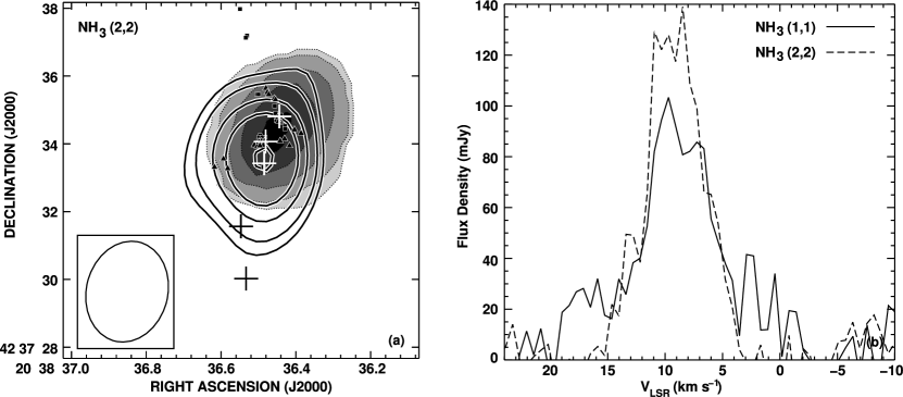
Figure 5: a) In greyscale levels we show the velocity-integrated (moment 0) emission from the (2,2) transition of ammonia. Levels are 50, 100, 200, 300, and 400 mJy beam^-1 km s^-1. The thin contours show the 1.3 cm emission continuum from the region (obtained from the line-free channels). Contours are -3, 3, 4, 6, 8, and 12 times 1.7 mJy beam^-1, the rms of the continuum image. The five crosses mark the positions of the continuum sources. The squares are the positions of the H₂O masers from Torrelles et al. (1997) and the triangles the OH masers from Hutawarakorn et al. (2002). The beam ($2\hbox to0.0pt{.\hss}{{}^{\prime\prime}}97\times 2\hbox to0.0pt{.\hss}{{}^{\prime\prime}}43$; PA = $-13^{\circ}$) is shown in the bottom left corner. b) Spectra of the (1,1) and (2,2) transitions of ammonia integrated over the region of emission. Lines are broad, and in the (1,1) spectrum the emission of the main line appears blended with that of the inner satellites.

In Figure 5 we investigate in more detail the region of active star formation. In the left panel of this Figure we show in greyscale the velocity-integrated (moment 0) emission of the (2,2) transition as well as the adjacent continuum emission, obtained from the line-free channels, in contours. On the right panel of this Figure we show the (1,1) and (2,2) spectra integrated over the region of emission. From this spectra we conclude that there is strong and broad (FWHM of $\sim$6 km s^-1) ammonia emission originating from the region that contains the continuum sources VLA 1, VLA 2, and VLA 3. This emission is most probably tracing dense ($\geq 3\times 10^{4}$ cm^-3) gas. ¿From the ratio of the inner satellite lines to the main line of the (1,1) transition ($\sim$0.3), we conclude that the emission is optically thin. Following Anglada et al. (1995) and assuming a $[NH_{3}/H_{2}]$ ratio of $10^{-7}$, we estimate a mass of $\sim$0.6 $M_{\odot}$ for the condensation.

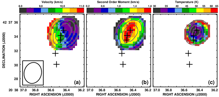
Figure 6: a) Velocity field (moment 1) from the (2,2) transition of ammonia. The color wedge at the top gives the LSR radial velocity in km s^-1. The beam ($2\hbox to0.0pt{.\hss}{{}^{\prime\prime}}97\times 2\hbox to0.0pt{.\hss}{{}^{\prime\prime}}43$; PA = $-13^{\circ}$) is shown in the bottom left corner. In all panels the contours mark the integrated emission (moment 0) of the (2,2) emission, contours are 50, 100, 200, 300, and 400 mJy beam^-1 km s^-1. The crosses mark the positions of the five radio sources. b) Velocity dispersion (moment 2) of the (2,2) emission. For a Gaussian line the FWHM is 2.35 times the value of the velocity dispersion. c) Rotational temperature of the gas, estimated from the (2,2)/(1,1) ratio, assuming optically thin emission and constant excitation conditions along the line of sight. The color wedge at the top gives the temperature in K.

In Figure 6 we show, on the left panel, the velocity field (moment 1) from the (2,2) transition. On the center we show the velocity dispersion (moment 2) from the (2,2) transition. For a Gaussian profile the full width at half power equals the dispersion multiplied by 2.35. Finally, on the right panel we show the rotational temperature of the gas. The region with ammonia emission shows a velocity shift of about 2 km s^-1 over a region of $\sim$3”. This velocity shift could be arising from different gas components associated with the multiple sources (VLA1, VLA2, VLA3) within the NH₃ beam. The central panel of Figure 6 indicates that the broadest emission overlaps the position of the sources VLA 1, 2, and 3. The right panel of Figure 6 indicates that the coolest parts of the ammonia cloud, with temperatures of about 35 K, overlaps the position of VLA 1.

2.3 X-ray Emission

Chandra/ACIS level 2 event data were extracted from Chandra archive (ObsID 8893, observed in 2008 February 2). The data were reduced with the ciao 3.4 data analysis system and the Chandra Calibration Database (caldb 3.4.0). The exposure time was processed to exclude background flares, using the task lc_clean.sl in source-free sky regions of the same observation.

Although the default pixel size of Chandra/ACIS detector is $\sf{0.492\arcsec}$, smaller spatial scales are accessible as the image moves across the detector pixels during the telescope dither, thus sampling pixel scales smaller than the default pixel of Chandra/ACIS detector. It allows us to create 0.125″  sub-pixel binning images. Furthermore, we applied adaptive smoothing CIAO tool csmooth, based on the algorithm developed by Ebeling et al. (2006) to detect the low contrast diffuse emission (minimum and maximum significance S/N level of 3 and 4, and a scale maximum of 2 pixels).

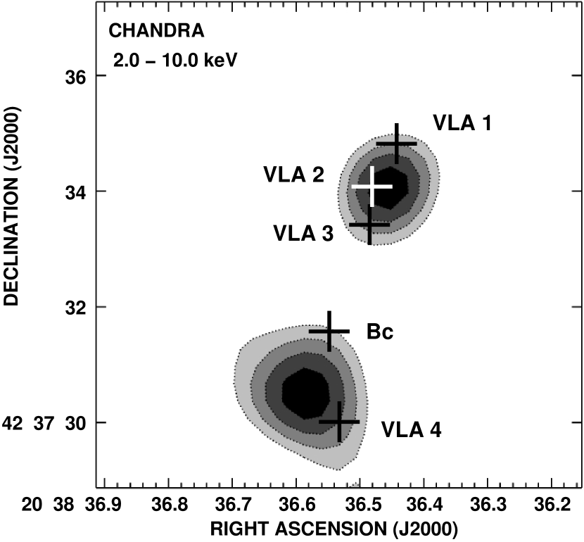
Figure 7: Left: Chandra/ACIS greyscale image of the 2.0 - 10.0 keV emission from the W75N region. Succesive greyscale levels are 0.05, 0.06, 0.07, and 0.08 counts/pixel. The crosses mark the positions of the five radio sources.

Three energy bands images were created: 0.2-10, 0.2-2 and 2-10 keV bands. We detected two sources; in spite of their low count rate ($2.0\times 10^{-4}$ and $2.7\times 10^{-4}$ count/sec), it is clear that they show emission only above 2 keV. This may indicate a very obscured environment ($\rm{N_{H}}\geq 10^{22}$ cm^-2), although high quality data are needed in order to confirm this possibility. An image from the 2.0 – 10.0 keV emission is shown in Figure 7. The two detected sources could be marking the positions of termination shocks of the outflows of the cluster of sources in W75N. Better data are required to determine the nature of the X-ray emission.

3 Discussion

3.1 Bc: a radio HH object

As commented in Section 2.1, the source Bc shows changes in its position, flux density and morphology. The source seems to be moving to the south with a velocity larger than 200 km s^-1 while it breaks into two components and dramatically increases its total flux density. This behavior is similar to that observed in optical (Devine et al. 2009) and radio (Curiel et al. 1993) Herbig-Haro objects, and, therefore, we interpret source Bc as an obscured radio HH object. Its radio luminosity (3.3 mJy in 2006, at a distance of 2 kpc) makes it one of the brightest HH objects detected in the radio. It is comparable to, but significantly above, HH 80 and HH 81 that have centimeter flux densities of 1-2 mJy at a distance of 1.7 kpc (Martí et al. 1993). The radio luminosity of source Bc is exceeded only by the radio HH objects associated with the luminous protostar IRAS 16547-4247, that with flux densities of $\sim$3-4 mJy at a distance of 2.9 kpc (Rodríguez et al. 2008) are the brightest known.

The radio flux density from source Bc allows to make an estimate of the mechanical luminosity of the jet that drives this source. Assuming that the continuum emission is optically-thin free-free at an electron temperature of $10^{4}$ K, and taking into account that the source is at a distance of 2 kpc, in the order of $\sim 1.1\times 10^{45}$ ionizations per second are needed to maintain the source ionized. If these ionizations have a collisional origin and assuming that a minimum energy of 13.6 eV is needed per ionization, a mechanical luminosity of $L_{mech}\geq 6~{}L_{\odot}$ is estimated. Finally, assuming that the jet has a velocity of $\sim 200$ km s^-1, a mass loss rate of order $10^{-6}~{}M_{\odot}$ yr^-1 is inferred for the jet that is producing source Bc.

3.2 VLA 2, VLA 3, and VLA 4

These results lead to a revision of the nature of the radio sources in W75N. As commented above, Source Bc is most probably a bow shock produced by a jet. Several arguments suggest that this jet is driven by VLA 3: i) the source Bc and possibly VLA 4 move away from VLA 3, and this source is elongated in the direction of motion, ii) the spectral index is consistent with that expected for a radio jet, and iii) VLA 3 is the only source that has associated SiO emission (presumably tracing an outflow) and associated 7 mm (Shepherd et al. 2004) and 1 mm (Shepherd 2001) continuum emission, suggesting association with a disk or envelope.

VLA 4 is either an independent star or could be a previous ejection from VLA 3. Unfortunately, VLA 4 is not detected at 3.6 cm in 1992 or 1998, but a comparison of the 3.6 cm data from 2006 and of the 2 cm data from 2001 suggests a small displacement to the south. New sensitive observations are needed to test this hypothesis.

Finally, VLA 2 is most probably an independent, very young star. This source was associated with the very strong OH flare emission that reached in 2003 an emission of about 1000 Jy to become the brightest galactic OH maser in history (Alakoz et al. 2005; Slysh & Migenes 2006).

3.3 What is the Nature of VLA 1?

Under the light of these results, one could propose that VLA 1 is the northern bow shock produced by the VLA 3 jet. However, in contrast to source Bc, VLA 1 does not show detectable proper motions along the axis of the VLA 3 jet. This behavior could be due to the existence of dense gas to its north that blocks motion along that direction. In fact, as shown previously, VLA 1 is associated with dense gas traced by the NH₃ observations. VLA 1 does show, however, a displacement in the peak of emission from east to west (see Fig. 2), nearly perpendicular to the axis of VLA 3 and similar to that observed in the radio HH objects associated with IRAS 16547-4247 (Rodríguez et al. 2008). In this latter source, this kinematic behavior has been interpreted as working surfaces where a precessing jet is interacting with a very dense medium. In this case, the HH objects would trace the present point of interaction between the jet and the dense medium.

We think, however, most likely that VLA 1 simply traces an independent young massive star. This source is known to be associated with intense maser emission from several molecules: water vapor (e.g., Lekht et al. 2009), methanol (e.g., Surcis et al. 2009), and hydroxil (e.g. Fish & Reid 2007). Intense maser emission is usually tracing the nearby presence of a young high-mass star. The proper motions observed in the water masers along the major axis of the VLA 1 source also favor this scenario (Torrelles et al. 2003). The linear polarization of the methanol masers revealing a tightly ordered magnetic field over more than 2000 AU around VLA 1 with a strength of 50 mG gives further support to the hypothesis that VLA 1 harbors a massive young star (Surcis et al. 2009). It is relevant to note that the flux density of VLA 1 remained constant within the noise during the three epochs of 3.6 cm observations, with all values consistent with 4.0$\pm$0.2 mJy.

4 Conclusions

We have analyzed VLA and Chandra archive data of the W75N region. In the radio continuum, we detect five sources: VLA1, VLA2, VLA3, Bc, and VLA4, from north to south respectively. Our main conclusions follow:

1) We detect important changes in total flux density, morphology, and position in the source Bc, suggesting that it is not tracing an independent star but actually is a radio HH object powered by VLA 3. Its average velocity in the plane of the sky is 220$\pm$70 km s^-1. If our interpretation is correct, this is one of the brightest radio HH objects known.

2) We detect J = 1–0; v = 0 emission of SiO centered on VLA 3, probably tracing the inner parts of an outflow associated with this radio jet. Our results strongly support the identification of VLA 3 as a radio jet.

3) The large scale ammonia emission shows that the W75N region contains two filamentary molecular clouds with different radial velocities. The star formation is taking place at the intersection of these two filaments, which is also the hottest region. This suggests that the star formation could be triggered by the collision of the two filamentary clouds.

4) Strong and broad (1,1) and (2,2) ammonia emission is detected from the region containing the radio sources VLA 1, VLA 2, and VLA 3.

5) We detected a new radio continuum component, VLA 4, a few arcsec to the south of the group of previously known sources.

6) Two sources are detected in the 2-10 keV band Chandra/ACIS image. These two sources could be tracing the termination shocks of outflows in the region, but better data are needed to understand the nature of the X-ray emission.

Figure 1: VLA contour images of the 3.6 cm (left) and 2 cm (right) emission from the W75N region. The contours are -4, 4, 6, 8, 10, 12, 15, 20, 30, 40, 50, and 60 times 45 and 78 $\mu$Jy beam^-1, the respective rms noises. The half power contours of the synthesized beams are shown in the bottom left corner of each figure and are $0\hbox to0.0pt{.\hss}{{}^{\prime\prime}}22\times 0\hbox to0.0pt{.\hss}{{}^{\prime\prime}}17;PA=18^{\circ}$ for the 3.6 cm image and $0\hbox to0.0pt{.\hss}{{}^{\prime\prime}}47\times 0\hbox to0.0pt{.\hss}{{}^{\prime\prime}}39;PA=-83^{\circ}$ for the 2 cm image. Both images were made with ROBUST = 0 (u,v) weighting. The source VLA 4 is a new detection. The epochs of the observations are given in the figure.

Figure 2: VLA contour images of the 3.6 cm emission for the three epochs (1992.90, 1998.23, and 2006.38) analyzed. Contours are -4, 4, 5, 6, 8, 10, 12, 15, 20, 25, and 30 times 80 $\mu$Jy beam^-1. The images have been restored with a circular beam of $0\hbox to0.0pt{.\hss}{{}^{\prime\prime}}25$, shown in the bottom left corner of the images. The crosses mark the centroids of the radio sources for epoch 2006.38. The source VLA 4 is detected only in the last epoch and it is not included in these images.

Figure 4: Superposition of the natural-weight images of the moment 0 of the NH₃(1,1) emission (contours) over the temperature image (colors). The solid contours trace the emission integrated in the velocity range from 5 to 8 km s^-1, while the dashed contours are integrated in the velocity range from 9 to 13 km s^-1. Contour levels are 30, 50, 100 and 200 mJy beam^-1 km s^-1. The color scale indicates the rotational temperature, as derived from the (2,2)/(1,1) ratio. The crosses mark the positions of the five continuum sources. The beam ($4\hbox to0.0pt{.\hss}{{}^{\prime\prime}}1\times 3\hbox to0.0pt{.\hss}{{}^{\prime\prime}}$; PA = $-18^{\circ}$) is shown in the bottom left corner of the image.

Table 1: Parameters of the VLA observations.

		Configuration/	Frequency	Flux	Phase Calibrator/	On-source	Calibration	Syntesized	RMS
Project	Epoch	Mode	(GHz)	Calibrator	Bootstrapped Flux Density (Jy)	Time (min)	Cycle (min)	Beama	(mJy)
AT141	1992 Nov 24 (1992.90)	A/Continuum	8.44	0137+331	2007+404/3.18$\pm$0.07	5.3	8	$0\hbox to0.0pt{.\hss}{{}^{\prime\prime}}23\times 0\hbox to0.0pt{.\hss}{{}^{\prime\prime}}19;-56^{\circ}$	0.09
AA224	1998 Mar 26 (1998.23)	A/Continuum	8.46	1331+305	2025+337/4.73$\pm$0.08	2.3	4	$0\hbox to0.0pt{.\hss}{{}^{\prime\prime}}24\times 0\hbox to0.0pt{.\hss}{{}^{\prime\prime}}20;48^{\circ}$	0.13
AS678	2000 Apr 24 (2000.31)	C/Line	43.4	1331+305	2012+464/1.07$\pm$0.02	196.4	2	$1\hbox to0.0pt{.\hss}{{}^{\prime\prime}}21\times 1\hbox to0.0pt{.\hss}{{}^{\prime\prime}}06;52^{\circ}$	3.2
AM652	2000 Aug 03 (2000.59)	D/Line	23.7	1331+305	2007+404/2.30$\pm$0.03	51.5	15	$2\hbox to0.0pt{.\hss}{{}^{\prime\prime}}97\times 2\hbox to0.0pt{.\hss}{{}^{\prime\prime}}43;-13^{\circ}$	6.6
AF381	2001 Apr 23 (2001.31)	B/Continuum	14.9	1331+305	2015+371/2.21$\pm$0.01	68.5	4	$0\hbox to0.0pt{.\hss}{{}^{\prime\prime}}47\times 0\hbox to0.0pt{.\hss}{{}^{\prime\prime}}39;-83^{\circ}$	0.08
AS831	2006 May 18 (2006.38)	A/Continuum	8.46	1331+305	2007+404/2.30$\pm$0.01	50.7	12	$0\hbox to0.0pt{.\hss}{{}^{\prime\prime}}22\times 0\hbox to0.0pt{.\hss}{{}^{\prime\prime}}17;18^{\circ}$	0.05

Table 2: Parameters of the continuum sources.

			Deconvolved Sizea	$S_{\nu}$(3.6 cm)b	$S_{\nu}$(2 cm)b	Spectral
Source	$\alpha$(2000)a	$\delta$(2000)a	(${}^{\prime\prime}\times^{\prime\prime};~{}^{\circ}$)	(mJy)	(mJy)	Indexc
VLA 1	$20^{h}~{}38^{m}~{}36\hbox to0.0pt{.\hss}^{s}445$	$+42^{\circ}~{}37^{\prime}~{}34\hbox to0.0pt{.\hss}{{}^{\prime\prime}}82$	0.43$\pm$0.02$\times$0.17$\pm$0.02; 80$\pm$2	3.8$\pm$0.1	3.0$\pm$0.2	-0.4$\pm$0.1
VLA 2	$20^{h}~{}38^{m}~{}36\hbox to0.0pt{.\hss}^{s}482$	$+42^{\circ}~{}37^{\prime}~{}34\hbox to0.0pt{.\hss}{{}^{\prime\prime}}08$	$<0\hbox to0.0pt{.\hss}{{}^{\prime\prime}}2$	0.7$\pm$0.1	2.4$\pm$0.3	2.2$\pm$0.3
VLA 3	$20^{h}~{}38^{m}~{}36\hbox to0.0pt{.\hss}^{s}486$	$+42^{\circ}~{}37^{\prime}~{}33\hbox to0.0pt{.\hss}{{}^{\prime\prime}}44$	0.21$\pm$0.01$\times$0.07$\pm$0.01; 157$\pm$3	4.0$\pm$0.1	5.7$\pm$0.2	0.6$\pm$0.1
Bc	$20^{h}~{}38^{m}~{}36\hbox to0.0pt{.\hss}^{s}549$	$+42^{\circ}~{}37^{\prime}~{}31\hbox to0.0pt{.\hss}{{}^{\prime\prime}}57$	0.75$\pm$0.05$\times$0.23$\pm$0.03; 74$\pm$3	3.3$\pm$0.2	3.0$\pm$0.3	-0.2$\pm$0.2
VLA 4	$20^{h}~{}38^{m}~{}36\hbox to0.0pt{.\hss}^{s}535$	$+42^{\circ}~{}37^{\prime}~{}30\hbox to0.0pt{.\hss}{{}^{\prime\prime}}03$	$<0\hbox to0.0pt{.\hss}{{}^{\prime\prime}}2$	0.7$\pm$0.1	0.9$\pm$0.2	0.4$\pm$0.5

References

- Alakoz et al. (2005) Alakoz, A. V., Slysh, V. I., Popov, M. V., & Val’Tts, I. E. 2005, Astronomy Letters, 31, 375
- Anglada et al. (1995) Anglada, G., Estalella, R., Mauersberger, R., Torrelles, J. M., Rodriguez, L. F., Canto, J., Ho, P. T. P., & D’Alessio, P. 1995, ApJ, 443, 682
- Baart et al. (1986) Baart, E. E., Cohen, R. J., Davies, R. D., Rowland, P. R., & Norris, R. P. 1986, MNRAS, 219, 145
- BHV (99) Ballesteros-Paredes, J., Hartmann, L. & Vázquez-Semanedi, E. 1999, ApJ, 527, 285
- Beltrán et al. (2001) Beltrán, M. T., Estalella, R., Anglada, G., Rodríguez, L. F., & Torrelles, J. M. 2001, AJ, 121, 1556
- Carrasco-González et al. (2006) Carrasco-González, C., López, R., Gyulbudaghian, A., Anglada, G., & Lee, C. W. 2006, A&A, 445, L43
- Choi (2005) Choi, M. 2005, ApJ, 630, 976
- Curiel et al. (1993) Curiel, S., Rodriguez, L. F., Moran, J. M., & Canto, J. 1993, ApJ, 415, 191
- Devine et al. (2009) Devine, D., Bally, J., Chiriboga, D., & Smart, K. 2009, AJ, 137, 3993
- Eb (06) Ebeling, H., White, D.A., & Rangarajan, F.V.N. 2006, MNRAS, 368, 65
- Eisloffel et al. (2000) Eisloffel, J., Mundt, R., Ray, T. P., & Rodriguez, L. F. 2000, Protostars and Planets IV, 815
- Feigelson & Montmerle (1999) Feigelson, E. D., & Montmerle, T. 1999, ARA&A, 37, 363
- Fischer et al. (1985) Fischer, J., Sanders, D. B., Simon, M., & Solomon, P. M. 1985, ApJ, 293, 508
- Fish & Reid (2007) Fish, V. L., & Reid, M. J. 2007, ApJ, 656, 952
- Galván-Madrid et al. (2010) Galván-Madrid, R., et al. 2010, in preparation
- Garay et al. (1996) Garay, G., Ramírez, S., Rodríguez, L. F., Curiel, S., & Torrelles, J. M. 1996, ApJ, 459, 193
- Haschick et al. (1981) Haschick, A. D., Reid, M. J., Burke, B. F., Moran, J. M., & Miller, G. 1981, ApJ, 244, 76
- Henriksen et al. (1991) Henriksen, R. N., Mirabel, I. F., & Ptuskin, V. S. 1991, A&A, 248, 221
- Ho & Townes (1983) Ho, P. T. P., & Townes, C. H. 1983, ARA&A, 21, 239
- Hunter et al. (1994) Hunter, T. R., Taylor, G. B., Felli, M., & Tofani, G. 1994, A&A, 284, 215
- Hutawarakorn et al. (2002) Hutawarakorn, B., Cohen, R. J., & Brebner, G. C. 2002, MNRAS, 330, 349
- Lekht et al. (2009) Lekht, E. E., Slysh, V. I., & Krasnov, V. V. 2009, Astronomy Reports, 53, 420
- Marti et al. (1993) Marti, J., Rodriguez, L. F., & Reipurth, B. 1993, ApJ, 416, 208
- O’Dell & Wong (1996) O’Dell, C. R., & Wong, K. 1996, AJ, 111, 846
- Persi et al. (2006) Persi, P., Tapia, M., & Smith, H. A. 2006, A&A, 445, 971
- RBM (08) Rodón, J.A., Beuther, H., Megeath, S.T., & van der Tak, F.F.S. 2008, A&A, 490, 213
- Rodríguez et al. (2008) Rodríguez, L. F., Moran, J. M., Franco-Hernández, R., Garay, G., Brooks, K. J., & Mardones, D. 2008, AJ, 135, 2370
- Shepherd (2001) Shepherd, D. S. 2001, ApJ, 546, 345
- Shepherd et al. (2003) Shepherd, D. S., Testi, L., & Stark, D. P. 2003, ApJ, 584, 882
- Shepherd et al. (2004) Shepherd, D. S., Kurtz, S. E., & Testi, L. 2004, ApJ, 601, 952
- Slysh & Migenes (2006) Slysh, V. I., & Migenes, V. 2006, MNRAS, 369, 1497
- Surcis et al. (2009) Surcis, G., Vlemmings, W. H. T., Dodson, R., & van Langevelde, H. J. 2009, A&A, 506, 757
- Torrelles et al. (1997) Torrelles, J. M., Gómez, J. F., Rodríguez, L. F., Ho, P. T. P., Curiel, S., & Vázquez, R. 1997, ApJ, 489, 744
- Torrelles et al. (2003) Torrelles, J. M., et al. 2003, ApJ, 598, L115
- VG (07) Vázquez-Semanedi, E., Gómez, G.C., Jappsen, A.K., Ballesteros-Paredes, J., González, R.F., & Klessen, R.S. 2007, ApJ, 657, 870
- Zapata et al. (2004) Zapata, L. A., Rodríguez, L. F., Kurtz, S. E., & O’Dell, C. R. 2004, AJ, 127, 2252