The SAGE-Spec Spitzer Legacy program: The life-cycle of dust and gas in the Large Magellanic Cloud

Abstract

The SAGE-Spec Spitzer Legacy program is a spectroscopic follow-up to the SAGE-LMC photometric survey of the Large Magellanic Cloud carried out with the Spitzer Space Telescope. We present an overview of SAGE-Spec and some of its first results. The SAGE-Spec program aims to study the life cycle of gas and dust in the Large Magellanic Cloud, and to provide information essential to the classification of the point sources observed in the earlier SAGE-LMC photometric survey. We acquired 224.6 hours of observations using the InfraRed Spectrograph and the SED mode of the Multiband Imaging Photometer for Spitzer. The SAGE-Spec data, along with archival Spitzer spectroscopy of objects in the Large Magellanic Cloud, are reduced and delivered to the community. We discuss the observing strategy, the specific data reduction pipelines applied and the dissemination of data products to the scientific community. Initial science results include the first detection of an extragalactic “21 $\mu$m” feature towards an evolved star and elucidation of the nature of disks around RV Tauri stars in the Large Magellanic Cloud. Towards some young stars, ice features are observed in absorption. We also serendipitously observed a background quasar, at a redshift of $z\approx 0.14$, which appears to be host-less.

1. Introduction

A photometric survey in the infrared of the Large Magellanic Cloud (LMC) was performed by the Spitzer Legacy Program Surveying the Agents of Galaxy Evolution (SAGE-LMC; Meixner et al., 2006), which charts the budget of gas and dust contributing to the cycle of star formation and stellar death in the Magellanic Clouds. Here we discuss SAGE-Spec, a spectroscopic follow-up to SAGE-LMC, which is also a Spitzer Legacy Program. For SAGE-Spec we observed a variety of circumstellar and interstellar environments with the Infrared Spectrograph (IRS; Houck et al., 2004) aboard Spitzer (Werner et al., 2004), as well as the SED mode available on the Multiband Imaging Photometer for Spitzer (MIPS; Rieke et al., 2004). The SAGE-Spec dataset is exceptionally suited to address the following issues: First, it allows us to trace the lifecycle of dust and molecular gas on its journey through the galaxy, from dust production sites (AGB stars, red supergiants, post-AGB-objects, planetary nebulae), to the ISM (atomic and molecular clouds) to star forming regions (H II regions, young stellar objects); and, second, it allows us to develop a photometric color-color and color-magnitude classification scheme to increase the legacy of the larger SAGE-LMC database. In addition, a large number of smaller astrophysical questions can be addressed using the data set provided here, and a rich harvest in scientific results is expected.

This paper gives an overview of the SAGE-Spec Legacy program. We outline the observing strategy, describe the data reduction process and discuss the data products that are currently publicly available to the astronomical community (Woods et al., 2010), or will become publicly available in the near future. Existing surveys targeting gas and dust in the LMC are discussed in Sect. 2. This section also includes a description of existing publications of infrared spectroscopy on LMC targets. The observing strategy of the SAGE-Spec project is discussed in Sect. 3, along with a description of the data reduction. This paper finishes with some first scientific results of the SAGE-Spec project (Sect. 4), and conclusions and an outlook to the future (Sect. 5).

2. Surveys: The gas and dust in the LMC

In order to study the life-cycle of dust on a galactic scale, the LMC provides a good compromise between distance and size. It is found at a distance of $\sim$50 kpc (Feast, 1999), and as an additional benefit has a favorable viewing angle (35^o, van der Marel & Cioni, 2001) resulting in low column densities, and typically just a single interstellar cloud, along each line-of-sight. It is possible to observe individual objects in the LMC due to its vicinity, while at the same time the outside viewpoint that we have enables us to obtain a global view of the LMC through surveys like this.

With $Z\approx 0.3-0.5\,Z_{\odot}$, the metallicity of the LMC is sub-solar (Westerlund, 1997). As a consequence the dust-to-gas mass ratio is $\sim$2–4 times lower than that in the Solar neighborhood (Gordon et al., 2003), permitting easier penetration of UV radiation to affect physical processes in the ISM and star formation. Indeed, modeling of photon-dominated regions shows that molecular clouds in the LMC will be larger and less dense than clouds in the Milky Way (Pak et al., 1998). The shape of the UV interstellar extinction curve appears to be independent of metallicity, thus constraining the differences between Galactic and LMC grain properties, although large variations exist between environments within the LMC (Misselt et al., 1999).

2.1. Surveys of the LMC

Previous infrared surveys of the stellar content of the LMC, performed with, for instance, MSX (Egan et al., 2001) and DENIS (Cioni et al., 2000), are limited to only the brightest sources. Exploration of the stellar content of the LMC was therefore skewed to the tip of the AGB and some bright supergiants. However, with its sensitive arrays, Spitzer has allowed for a full census of all objects brighter than $\sim 15^{\mathrm{th}}$ magnitude in the 8.0 $\mu$m band (Meixner et al., 2006). SAGE-LMC encompasses a field of $7^{\mathrm{o}}\times 7^{\mathrm{o}}$ covering the majority of the LMC, observed using all bands of the InfraRed Array Camera (IRAC; Fazio et al., 2004) and MIPS. The IRAC and MIPS point source catalog contains about 6 million sources, and has been made available to the community (Meixner et al., 2006). The post- and pre-Main Sequence populations uncovered by SAGE-LMC are discussed by e.g. Blum et al. (2006) and Whitney et al. (2008).

The extended emission component of the SAGE-LMC survey is discussed in more detail by Bernard et al. (2008), who include references to additional LMC surveys in molecular and atomic emission, e.g. H$\alpha$ (Gaustad et al., 2001), Hi (Kim et al., 2003; Staveley-Smith et al., 2003), and CO (Fukui et al., 2008). In addition, a full survey of OH maser emission in the LMC has been performed (Green et al., 2008), as well as photometric surveys in the optical (e.g. Massey, 2002; Zaritsky et al., 2004).

2.2. Mid-infrared spectroscopic studies

Several mid-infrared spectroscopic studies of representative targets in object classes in the LMC have already been performed. Most studies focus on individual objects or small samples, although a few systematic studies of large samples exist. Here we provide an overview of studies not including data from SAGE-Spec.

2.2.1 Silicates

Prior to the launch of Spitzer, Voors et al. (1999) obtained 2–45 $\mu$m spectroscopy of R71, a Luminous Blue Variable in the LMC, using the Short Wavelength Spectrometer (SWS; de Graauw et al., 1996) on board the Infrared Space Observatory (ISO; Kessler et al., 1996). This spectrum contained the first detection of extragalactic crystalline silicates, and also showed the presence of polycyclic aromatic hydrocarbons (PAHs).

With Spitzer-IRS the possibility to obtain mid-infrared spectroscopy of individual objects greatly expanded, allowing the analysis of the dust mineralogy. IRS spectroscopy of two B$[$e$]$ hypergiants (R126 and R66) revealed the presence of silicate dust, where R66 also shows evidence for crystalline silicates and a dual chemistry with the presence of PAHs (Kastner et al., 2006). Both of these sources are known to have disks, which may provide a suitable environment for crystallization. Additional sources found with a silicate mineralogy are IRAS 05003$-$6712, which shows the characteristic features of crystalline silicates enstatite and forsterite superposed on amorphous silicate features (Zijlstra et al., 2006), and HV 2310, a Mira-type star showing an unusually-shaped 10 $\mu$m resonance, which suggests the presence of both crystalline and amorphous silicates (Sloan et al., 2006a).

2.2.2 Carbon-rich and oxygen-rich evolved stars

The late-stage AGB stars that dominate the MSX 8-$\mu$m point source list (Egan et al., 2001) are almost exclusively carbon-rich, as is expected in the low metallicity environment of the LMC (e.g. Zijlstra et al., 2006; Sloan et al., 2008). The C₂H₂ molecular absorption bands are deeper than those in their Galactic analogs explained by a higher abundance of this species at low metallicity (Zijlstra et al., 2006). Particularly deep molecular absorption bands are found in IRAS 04496$-$6958 (Speck et al., 2006), along with a possible detection of SiC at 11.3 $\mu$m in absorption. Another object, SMP LMC 11, is classified as a planetary nebula based on its emission lines although its infrared spectral energy distribution is more reminiscent of a post-AGB star (Bernard-Salas et al., 2006). The spectrum of SMP LMC 11 shows a variety of organic molecular bands in absorption, including several first extragalactic detections. However, Matsuura et al. (2006) have performed a study of molecular bands (C₂H₂ and HCN) in a larger sample of carbon stars and find that the abundance of C₂H₂ is independent of metallicity, while the HCN bands remain undetected.

An inventory of dust features in the IRS spectra of carbon-rich AGB stars in the LMC is given by Zijlstra et al. (2006), and shows the presence of SiC and MgS solid state components. Leisenring et al. (2008) have added a further 19 sources to this sample, and devised a method to study the dust condensation sequence in environments of differing metallicity. It was also noted that the occurrence of MgS correlates with diminished strength of the SiC feature, suggesting that MgS forms a coating on SiC grains (Lagadec et al., 2007; Leisenring et al., 2008), although this seems contradictory with observations of a sample of 7 of the most extremely reddened carbon stars (Gruendl et al., 2008), where the presence of MgS apparently did not hamper the detection of SiC in absorption.

2.2.3 Planetary Nebulae

The prevalence of the carbon-rich phase in stellar evolution is supported by evidence from IRS observations of Planetary Nebulae (PNe). Stanghellini et al. (2007) have observed 41 PNe in both Magellanic Clouds, 25 of which are LMC sources, and which were previously observed using HST. Roughly half of the spectra of the LMC PNe are dominated by atomic emission lines, while the remainder show solid state features, of mostly carbon-rich species. Only two LMC PNe show clear detections of oxygen-rich dust, in particular crystalline silicates. An independent study of atomic lines performed on a sample of 25 LMC/SMC PNe yielded neon and sulfur abundances (Bernard-Salas et al., 2008), both of which are found to be lower than the Galactic values, roughly in the same ratios as the metallicity ratios with respect to the Milky Way.

2.2.4 Supernovae and their remnants

A detailed study of supernova remnant N132D by Tappe et al. (2006) included IRS observations and showed the emission lines of $[$Neiii$]$ and $[$Oiv$]$, as well as PAH emission features – including relatively strong emission from the PAH features at 14-20 $\mu$m. The observations were of part of the shell and a fast-moving knot. In supernova remnant N49 the PAH features are less prominent compared to the atomic emission lines (Williams et al., 2006), which may indicate PAH destruction by UV radiation. The IRS spectrum of recent supernova SN 1987A is dominated by emission from silicate dust, with a few atomic lines (Bouchet et al., 2006). The dust mass derived is $\sim 2.6\times 10^{-6}\,M_{\odot}$.

2.2.5 Pre-Main Sequence stars

IRAS 05328$-$6827 is the first YSO to be analyzed with the IRS in the LMC, showing a CO₂ ice band that, compared to the H₂O ice band, is deeper than that typically observed in the Milky Way (van Loon et al., 2005b). Seale et al. (2009) have targeted YSO candidates suggested by Gruendl & Chu (2009) and spectrally identified 277 YSOs, thus greatly expanding the sample of known YSOs in the LMC. These YSOs were subdivided in 6 different groups based on the presence of CO₂ ice features, silicate features, PAH features and atomic emission lines.

2.2.6 Spectral catalogs of point sources

A number of studies have compiled spectral catalogs. Spanning a range of infrared colors, Buchanan et al. (2006) have selected and observed 60 of the brightest 8 $\mu$m sources, and classified 21 red supergiants, 16 carbon-rich and 4 possible oxygen-rich AGB stars, 2 OH/IR stars and the 2 B$[$e$]$ stars discussed in Sect. 2.2.1. A smaller sample of 28 sources taken from a range of pre-defined classes is presented by Sloan et al. (2008) and reveals a veritable zoo of spectra. The classification scheme devised by Buchanan et al. (2006) has been used by Kastner et al. (2008) to classify 250 of the most luminous 8 $\mu$m MSX sources in the LMC, arriving at the conclusion that in this flux-limited sample carbon-rich AGB stars indeed dominate (35% of the sources), closely followed by H II regions (32%; some of which might contain massive YSOs), and at some distance Red Supergiants (18%). Less prominent in this sample are the populations of oxygen-rich AGB stars (5%), dusty early-type emission-line stars (3%) and foreground AGB stars (3%) in this sample. The remaining 4% of sources could not be classified. This classification was tested by (Buchanan et al., 2009), who found by studying the IRS spectra of objects which were not previously classified in their earlier work (Buchanan et al., 2006), that 22 out of 31 sources received the correct classification.

3. Observations

Table 1Summary of observations in the SAGE-Spec program

observing mode	number of targets	total obs. time
IRS staring	196 point sources	108.7 hrs
IRS mapping	10 atomic clouds	64.2 hrs
	10 H II regions
	20 background
MIPS SED	10 atomic clouds	20.5 hrs
	10 H II regions
	20 background
MIPS SED	48 point sources	31.2 hrs

The Spitzer SAGE-Spec program (PID: 40159) consists of 224.6 hours of spectroscopic observations of targets in the LMC (Tab. 1). The targets included point sources and extended regions, both of which were observed using the IRS low resolution and MIPS SED modes. Observations were done in the IRS staring mode for 196 point sources, and 48 point sources were observed in MIPS SED mode. In addition, 10 extended regions were mapped in both the MIPS SED and IRS observing modes. These SAGE-Spec data are discussed in Sect. 3.1 (point sources) and Sect. 3.2 (extended regions).

In addition to the observations made as part of the SAGE-Spec program, we also deliver to the scientific community our new, homogeneous reductions of all archival IRS and MIPS SED spectroscopic data within the SAGE-LMC footprint, as part of the SAGE-Spec legacy. Tab. 5 lists the archival IRS staring mode observations, while the archival IRS maps and MIPS SED observations within the SAGE-LMC footprint are discussed in Sect. 3.1.3 and Sect. 3.2.3.

3.1. Point sources

3.1.1 Target selection

Spectroscopic studies performed with Spitzer prior to the SAGE-LMC survey, in observing cycles 1–3, (e.g. Buchanan et al., 2006; Zijlstra et al., 2006) have predominantly targeted (extreme) AGB stars known before the launch of Spitzer. These objects are concentrated in the brightest part of the [8.0] vs. [8.0]-[24] color-magnitude diagram (blue triangles in Fig. 1), above the MSX detection limit.

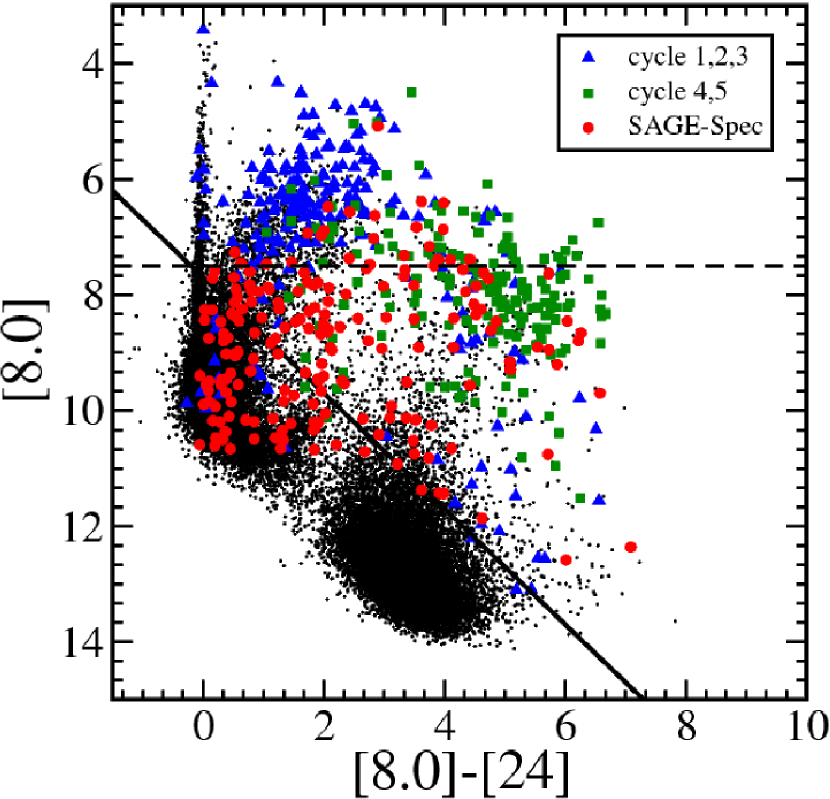
Figure 1.— [8.0] vs. [8.0]-[24] color-magnitude diagram of infrared point sources in the LMC. The black dots represent the sources for which these colors are available in the SAGE-LMC point source catalog (Meixner et al., 2006). Sources selected for observation in the SAGE-Spec program are indicated with red circles, whereas archival targets observed in cycles 1–3, and cycles 4–5 are shown as blue triangles and green squares, respectively. The latter group is dominated by targets from PID 40650 (PI: Looney; Seale et al., 2009). The diagonal solid line in the diagram represents the sensitivity limit that we applied to select sources for LL observations. SAGE-Spec sources below this line were only observed with SL. The MSX detection limit at 8.0 $\mu$m is shown as a horizontal dashed line.

In order to explore the full life-cycle of dust in the LMC and to classify completely the sources in the SAGE-LMC photometric catalogs, we have selected additional sources that cover the range in luminosities and colors found in the SAGE-LMC photometric survey, focusing predominantly on the unexplored region below the MSX detection limit, and including some additional bright, extremely red sources (red circles in Fig. 1). The SAGE-Spec program was executed in observing cycle 4, with the SAGE-LMC data becoming available to the SAGE-LMC/SAGE-Spec team and the community prior to the proposal deadline for that cycle. Several other proposals targeted point sources in the LMC below the MSX detection limit, most notably the program An Evolutionary Survey of Massive YSOs (PID: 40650; PI: L. Looney; Seale et al., 2009), in which about $\sim$300 candidate YSOs were targeted, selected from the SAGE-LMC observations using independent photometry from Gruendl & Chu (2009); so this area, too, received substantial coverage with IRS over the lifetime of Spitzer. The cycle 4 and 5 targets, dominated by the sample proposed by Seale et al. (2009), are marked with green squares in Fig. 1.

For the SAGE-Spec program, we arrived at a target list containing 196 pointings, all of which have been observed using the short low (SL) mode on IRS, while 128 of these were also observed in the long low (LL) mode (see Tabs. 3 and 4). We focused on field stars, but also included a small sample of objects from clusters with known metallicities and ages, yielding targets of a much better constrained pedigree than field stars. Cluster stars were mostly overlooked prior to the SAGE-Spec survey. The cluster sources are indicated as such in Tab. 3.

We selected candidates in a range of object classes. The sample includes candidate AGB stars, both O-rich and C-rich, selected from the work by Srinivasan et al. (2009); and potential YSO sources taken from the list of candidates selected on their colors and magnitudes (Whitney et al., 2008). Due to the overlapping color-magnitude space with YSOs, we also expected to detect background galaxies (Blum et al., 2006). In addition, we ensured representation of rarer objects, such as post-AGB stars and PNe using additional criteria. For the post-AGB stars the samples of Alcock et al. (1998) and Wood & Cohen (2001) provided a starting point; while the PNe were drawn from lists of LMC PNe assembled by Leisy et al. (1997) and Reid & Parker (2006), representing an adequate sampling of electron density and temperature, morphology, and infrared colors. In order to fully cover the color-magnitude space parametrized by IRAC, MIPS and 2MASS magnitudes, we selected a total of 13 sources from under-represented regions, such as the region defined by $[3.6]-[8.0]>5$ and the region bordered by $[8.0]>9$ and $J>13.3$. The distribution of the selected sources over the LMC is shown in Fig. 2.

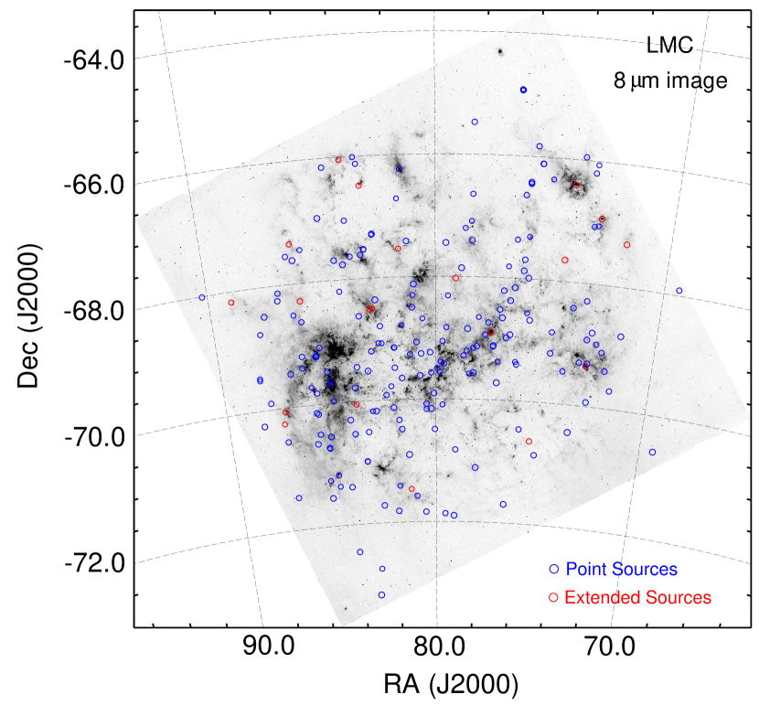
Figure 2.— Distribution of SAGE-Spec IRS targets over the LMC. The blue symbols indicate the positions of point sources targeted with the IRS staring mode, while the red symbols indicate the central positions of the 20 MIPS SED/IRS maps of extended regions. The positions are overplotted on the IRAC 8-$\mu$m footprint of the SAGE-LMC survey (Meixner et al., 2006)

MIPS SED point source target selection

We observed 48 point sources with MIPS SED (Tables 3 and 5), which is only feasible for the brightest objects in the LMC. A minimum flux level of 100 mJy at 70 $\mu$m is required to obtain a S/N of $\sim$3 for $20\times 10$s integrations. We also required all targets selected for MIPS SED observations to have been observed with IRS, either within the context of the SAGE-Spec program, or archival programs in cycle 1–3.

3.1.2 IRS staring mode

Observations

The IRS observations of the point sources in the sample are carried out in staring mode. All 196 selected targets were observed using IRS-SL, while the 128 targets with a MIPS-24 $\mu$m flux $\gtrsim 5.7$ mJy were also observed with IRS-LL. Each target was observed in both nod positions, located one-third and two-thirds along the slit. Integration times were chosen based on the IRAC-8.0 and MIPS-24 $\mu$m flux levels, and targeted to result in a S/N of 60 in SL and 30 in LL, in principle sufficient to analyze and classify dust features on top of a stellar continuum.

Although we observed toward 196 positions, one observation (AOR key 22402560) clearly showed the contribution of two different objects in SL and LL; at short wavelengths the spectrum is due to GV 60, present at the observed location, while the LL spectrum is dominated by nearby Wolf-Rayet star LH$\alpha$ 120–N 82.

Data reduction SAGE-Spec data

The processing of data for the SAGE-Spec program began with the flat-fielded images produced by the S18.7 version of the data-reduction pipeline at the Spitzer Science Center (SSC). To extract spectra from the flat-fielded images and calibrate them spectrophotometrically, we followed the procedure used by several other programs in the Magellanic Clouds and elsewhere in the Local Group (e.g.  Sloan et al., 2006b; Zijlstra et al., 2006; Lagadec et al., 2007; Matsuura et al., 2007; Sloan et al., 2008, 2009; Lagadec et al., 2009). The SL and LL modules each have two apertures, one for the second-order data covering the shorter-wavelength portion, and the other for the first-order data covering the longer-wavelength portion. When the target is in the second-order aperture (SL2 or LL2), a short piece of first-order data is also obtained, which is referred to as the bonus order (SL-bonus or LL-bonus). The bonus order provides overlap with the true first-order data (SL1 or LL1), making it possible to correct the spectra for discontinuities between the orders.

Observations were constructed so that the number and length of integrations in each aperture within a module matched, giving us flexibility on the background subtraction method. Generally, in SL, we chose as the background for a given exposure the corresponding exposure with the target in the other aperture. These aperture differences place the positive and negative beams about 79^′′ apart, compared to 19^′′ if we had used nod differences. In SL, nod differences would have placed the positive and negative beams close enough to each other to interfere for extended or complex sources. Consequently, we only reverted to nod differences for those observations where the background emission showed a gradient over the 79^′′ throw. For LL, the default for background subtraction was a nod difference, which placed the positive and negative beams $\sim$56^′′ apart. We generally avoided using aperture differences in LL because the beams were 192^′′ apart, which would often expose us to the more severe background gradients present in the LMC longward of 15 $\mu$m. We examined each image and spectrum carefully to assess when it was necessary to deviate from the default background-subtraction method to avoid either additional sources or complex backgrounds. In some cases, we even reverted to using the image with the target in the other aperture and nod as the background (a cross difference).

In addition to removing the background, differencing the data also corrects most of the rogue pixels in an image. These pixels exhibit dark currents different than their usual levels, but generally stable for the duration of a given observation. Some pixels remain problematic for a variety of reasons. Most are flagged as such in the rogue pixel masks provided by the SSC. We built super-rogue masks assuming that up to the campaign in which a target was observed, a pixel could be defined as bad if it had been flagged as bad in two previous campaigns. We replaced all flagged pixels using the imclean algorithm developed at Cornell and distributed as a part of irsclean by the SSC. This algorithm replaces bad pixels by comparing the point-spread functions (PSFs) in adjacent rows.

To extract spectra from the differenced and cleaned images, we used the SSC pipeline modules profile (to locate the source in the slit), ridge (to map the source position and extraction aperture in the image), and extract. The extract module extracts a spectrum from an image by summing the flux within a pseudo-rectangle defined for each wavelength element. When the boundaries of a pseudo-rectangle cross a pixel, the flux is assumed to be evenly distributed within that pixel. The pseudo-rectangles are centered on the center of the PSF at each wavelength element, and their width increases proportionally with wavelength. The tapered-column extraction within SMART (Higdon et al., 2004) was designed to follow this algorithm precisely, and it gives very similar results .

Spitzer obtains IRS data in a series of Data Collection Events (DCEs). We extracted spectra separately from each DCE, then co-added them to produce one spectrum per nod position. This step produces a mean flux density and a standard deviation, which we divided by the square root of the number of DCEs to estimate the uncertainty in flux density. To calibrate the co-added spectrum from each nod position, we determined spectral corrections using IRS observations of the standard stars HR 6348 (K0 III), HD 166780 (K4 III) and HD 173511 (K5 III). HR 6348 served as the standard for SL (to avoid any difficulties with the strong SiO absorption in the later K giants), while all three served as standards for LL (to maximize the S/N). We chose to use K giants rather than $\alpha$ Lac (A1 V; e.g. Furlan et al., 2006) because of the difficulty in predicting the strength of the hydrogen recombination lines in the low-resolution modules.

When combining the spectra from the two nod positions for a given order, we replaced the uncertainty when a comparison of the two spectra produced a larger value. When the uncertainty for a given pixel exceeded the average uncertainty in the neighborhood by a factor of five (typically), we used only the data from the nod which were closer to neighboring data. This spike-rejection algorithm removed the occasional spikes and divots which survived the cleaning step above.

Table 2Wavelength ranges

segment	wavelength ($\mu$m)
SL2	5.10–7.59
SL-bonus	7.23–8.39
SL1	7.59–14.20
LL2	13.95–20.54
LL-bonus	19.28–21.23
LL1	20.46–37.00

Finally, spectra from the six orders were combined into one spectrum (SL2, SL-bonus, SL1, LL2, LL-bonus, LL1; see Table 2). First the bonus-order data were averaged with the first- and second-order data where they overlapped and were within the defined range of valid data. Then the spectra were stitched together to remove discontinuities between segments. These discontinuities arose primarily from mispointings, almost always in SL, with its narrower slit (3.6^′′ vs. 10.0^′′). In general, we assumed that the corrections were always upward to the best-centered spectral segment. All corrections were multiplicative and scalar (i.e. not a function of wavelength). To conclude the processing, we trimmed the spectra of those portions at the ends of each segment which proved impossible to calibrate reliably. We also reset uncertainties which indicated a signal/noise ratio $>$ 500, as these values are unlikely and can adversely affect algorithms which use the S/N to weight the data.

Archival data

We have perused the archive for all staring mode observations within the SAGE-LMC footprint, and complemented this list with a few mini-map observations, apparently designed to target point sources. The observations are listed in Tab. 5. Most observations are single pointing staring mode observations, but in some cases more complex settings are used. Examples are the mini-maps, which appear to be designed to cover the entire point-spread-function, and cluster mode observations, where several pointings are strung together in a single AOR. All archival targets were reduced following the scheme described above. One target was only observed with SL2, forcing us to depart from our default background subtraction using aperture differences, since there is no other aperture to extract. For those data, and in other cases where complex backgrounds made aperture differences inadvisable, we used nod differences in SL.

We include both low-resolution (SL and LL) and high-resolution (SH and LH) in the final data delivery. Both Short-High (SH) and Long-High (LH) have short slits, which limit the background-subtraction method. Later in the Spitzer mission, the SSC strongly recommended that all SH and LH observations include dedicated background observations, but most observations early in the mission came with no background observations. Where these were available, we subtracted them from the images before extracting. When they were not, then we were forced to skip this important step and continue without background subtraction. In all cases, we performed a full-slit extraction, summing all of the flux in the slit at each wavelength. When stitching high-resolution data, we have not applied different corrections to the orders within SH or LH, because these were all obtained simultaneously and cannot differ due to pointing effects. Sample spectra showing the reduced IRS staring mode data are shown in Fig. 3.

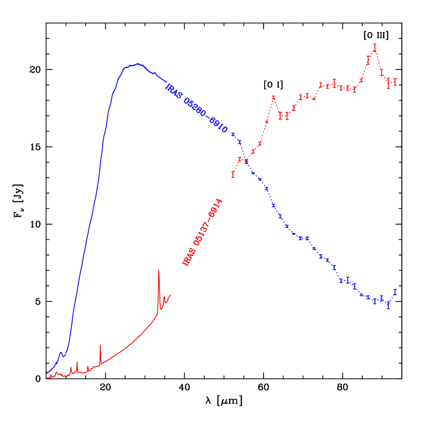
Figure 3.— Combined MIPS SED (van Loon et al., 2010) and IRS view of two bright, compact IR sources: one, OH/IR star IRAS 05280$-$6910 is dominated by a warm circumstellar dust envelope with the 10 and 18 $\mu$m silicate features in absorption and a declining, featureless continuum at far-IR wavelengths; the other, ultra-compact H II region IRAS 05137$-$6914 is dominated by cold dust and an emission-line spectrum both at mid- and far-IR wavelengths.

3.1.3 MIPS SED point sources

Observations

For the MIPS SED mode observations, the integration times are determined based on the measured 70 µm emission, from SAGE-LMC, and the slope of the SED. The chop size was chosen to place the background measurement in a region relatively free of emission for the range of dates expected for the observations. Due to the high efficiency of Spitzer scheduling, the MIPS SED observations were taken earlier than expected, resulting in some chop regions not being taken in the ideal locations. The chop sizes were normally $1^{\prime}$, except in five cases were a chop of either $2^{\prime}$ or $3^{\prime}$ was employed. Integration times ranged between 24 s and 200 s.

For the LMC, there is one additional point source with MIPS SED observations available in the Spitzer archive. This is SN 1987A and has been observed as part of programs 30067, 40149 & 50444 (PI: Dwek). The IRS spectroscopy and MIPS and IRAC photometry associated with these programs is already published (Bouchet et al., 2006).

Data Reduction

The MIPS SED point source observations were reduced using the MIPS DAT (see  Gordon et al., 2005). The extraction was done for a 5 pixel wide aperture centered on the collapsed profile maximum. For the majority of the sources, the off-source chop observations were used to do the initial background subtraction (except when there was significant emission in the off-source chop position). In addition, background subtraction was done by subtracting the measurements made with the same extraction aperture in a region near the edge of the slit. A wavelength dependent aperture correction was applied to extrapolate to infinite extraction aperture. Finally, a smoothed sensitivity function was applied to convert from instrumental to physical units. The uncertainty due to the absolute calibration is 15% (Lu et al., 2008). Fig. 3 shows the MIPS SED spectrum of point sources IRAS 05280$-$6910 and IRAS 05137$-$6914, as examples of the quality of the data. More details on, and first science results from, the MIPS SED observations of point sources in the LMC can be found in van Loon et al. (2010).

3.2. Extended regions

3.2.1 Target selection

For the interstellar extended source observations, we distinguish between highly irradiated (ionized) extended regions (i.e. H II regions) and lower-level irradiated clouds, described as atomic and molecular clouds. The H II regions in the SAGE-Spec program (see Tab. 6) have been selected on size and the r.m.s. density as derived from the H$\alpha$ emission (Kennicutt & Hodge, 1986). The source list covers a range in sizes from $1^{\prime}$ to $16^{\prime}$, while the electron density range spans about two orders of magnitude. H ii regions cover only part of IRAC/MIPS color-color space in the LMC (circles in Fig. 4). The atomic regions were selected from the $F_{8.0}/F_{24}$ and $F_{70}/F_{160}$ IRAC/MIPS color-color space, as observed by SAGE-LMC, and are chosen to span a wide range of these IRAC and MIPS colors (Fig. 4). Based on the overall pixel statistics, we divided the color-color space into a number of canonical bins (e.g. $5<F_{8.0}/F_{24}<10$ and $F_{70}/F_{160}<0.1$), and selected regions with high concentrations of pixel values in these bins. As an additional criterion we required these regions to have a distinct identity, for instance a feature in the Spitzer maps or a CO or H I cloud. The selection is somewhat exploratory in nature due to its small size.

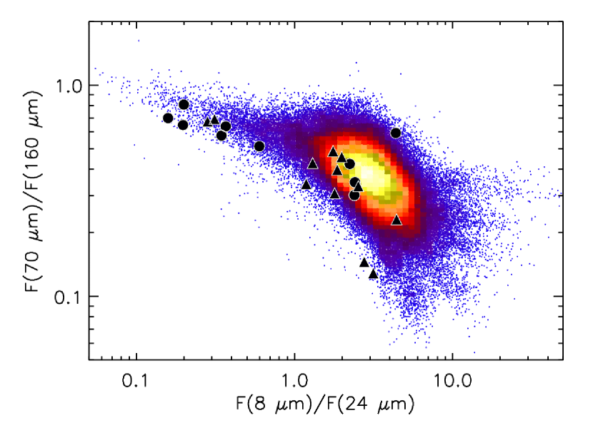
Figure 4.— IRAC/MIPS color-color diagram for extended regions. The SAGE-LMC data for all three MIPS bands and the IRAC 8-$\mu$m band were convolved to the spatial resolution of the MIPS-160 $\mu$m band. The background dots represent the ratios of these bands for each MIPS-160 spatial resolution element. The H II regions that were observed for the SAGE-Spec program are plotted as circles and the diffuse regions as triangles.

While the H II regions in general tend toward $F_{8}/F_{24}$ ratio $\sim$ 1, the atomic regions chosen span higher ratios ranging from 1 to 10, on average. This selection does not guarantee that H II regions are not present in the atomic regions mapped, but samples regions which would be dominated by properties characteristic of atomic ISM. The SAGE-Spec sample has been extended by the archival IRS and MIPS SED maps of the 30 Doradus H II region (Indebetouw et al., 2009) and two additional atomic regions in the LMC from PID 40031 (PI: G. Fazio; SSDR 11 and SSDR 12 in Tab. 6), of which the data remain unpublished so far. The central positions and sizes of all 23 extended regions are listed in Tab. 6.

3.2.2 IRS mapping mode

Observations

For the atomic and molecular cloud observations, our sensitivity objective was to obtain spectral maps such that when spatially integrated over a $1\arcmin\times 1\arcmin$ region, we would achieve a S/N = 10. We used exposure times per pixel of $4\times 14$s (SL) and $4\times 30$s (LL) and spectral mapping to cover each $1\arcmin\times 1\arcmin$ region. All selected H II regions are mapped in strips that have a width of $1\arcmin$, and the length being the diameter of the H II region. The mapping is done in such a way that the SL slit is stepped in the cross-slit direction by the diameter of the H II region and contains 2 pointings in the slit direction. The LL slit is stepped in the cross-slit direction by $1\arcmin$ and again in the slit direction by the diameter of the H II region, thus obtaining a $1\arcmin$ wide strip in both LL and SL. There are four 6s exposures for both modules, and, since the maximum length of an IRS AOR is 6 hours, the total length of the strip is limited to 5.4^′. The largest H II regions in our sample are therefore not mapped to their full diameter. For both the low surface brightness clouds and the H II regions, dedicated off-source observations were obtained to remove the time dependent IRS detector hot pixels and zodiacal light background.

Data Reduction

We used the standard pipeline data as produced by the SSC. The individual observations were combined into a spectral cube using CUBISM (Smith et al., 2007a), and these spectral cubes were merged together using custom software (Sandstrom et al., 2009). Each independent spectrum in the cube was fit using PAHFIT (Smith et al., 2007b) after convolution to a common resolution using custom convolution kernels (Gordon et al., 2008; Sandstrom et al., 2009). The fit parameters are used to construct the feature maps. For the molecular and atomic regions, we did achieve a S/N of 10, especially at $\lambda>10$ $\mu$m. For the H II regions, more mixed results emerged, with only 6 of the 10 regions meeting the S/N goal. In those regions with a S/N $>10$ it is possible for us to investigate spatial variations in the properties of dust and PAHs, and correlate this with the interstellar radiation field measured through PAH feature strengths and atomic line ratios.

We have also spatially integrated the IRS (and MIPS SED) spectroscopy, as Fig. 5 shows for one of the atomic regions. The integrated SED of this region was extracted from the individual IRS order cubes and MIPS SED cube over the region in common between all the observations. In this example, the extracted region was a 60^′′ diameter circle. When studying spatial variations is not possible due to low S/N, the integrated spectra still yield global information on the dust and PAH properties, and the radiation fields in these environments.

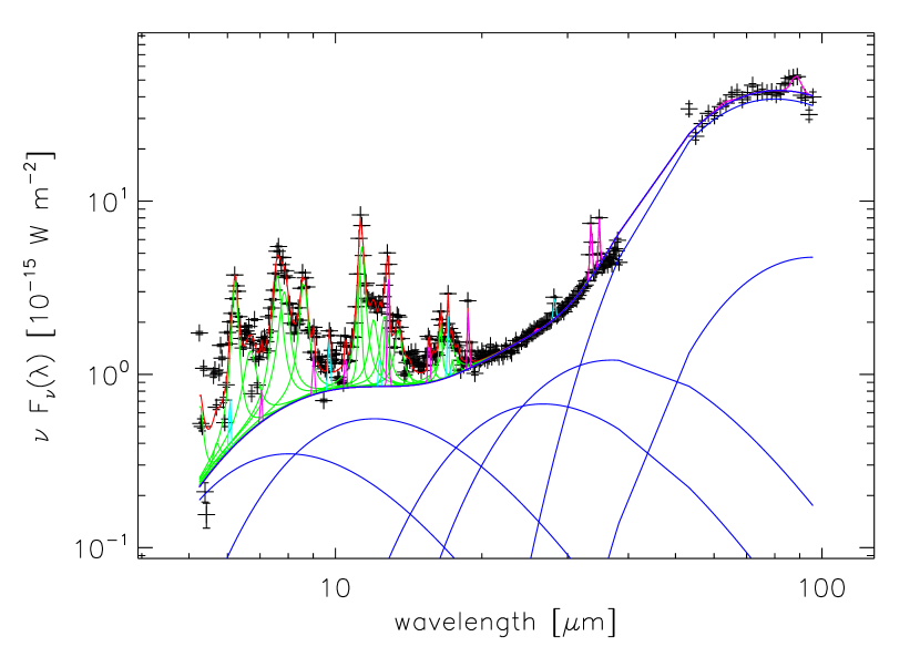
Figure 5.— Integrated IRS and MIPS SED spectrum of SSDR 1. The spectrum is spatially integrated over a circle with diameter 60$"$, centered on the position listed in Tab. 6. A modified form of the PAHFIT model has been applied (see main text). The pluses indicate the data, and the solid lines are the various components of the PAH fit model, with blue representing the dust continuum, cyan the atomic transitions, and green the PAH bands. The overall fit is indicated with a red line.

3.2.3 MIPS SED

Observations

For the H II regions, the MIPS SED observations roughly coincide with the peak of the SED and pick up any strong [O I] 63 µm and [O III] 88 µm lines (Indebetouw et al., 2009). For the atomic and molecular regions the MIPS SED observations constrain dust temperatures, and, in particular, the very small grain emission properties. All SAGE-Spec extended regions are mapped with 1/2 slit offsets in both slit dimensions (9^′′ cross-slit and 1.25^′′ along-slit), with the minimum exposure time of 3 s. With these exposure times, we aimed to achieve a S/N of 5 per spatial bin for the H II regions, while for the diffuse regions, the objective is for a S/N of 5 for the spatially integrated SED ($1\arcmin\times 1\arcmin$ region). Indeed, these S/N goals were met for 7 out of 10 H II regions, and all of the diffuse regions. For all extended regions, dedicated background observations off the LMC were obtained.

For the LMC, there are two additional extended sources with MIPS SED observations available in the Spitzer archive. They are 30 Dor (Indebetouw et al., 2009); and the 70 µm excess (as described by Bernard et al., 2008) region observed in PID 40031, for both of which IRS mapping mode observations are also available (see Sect. 3.2.2).

Data Reduction

The MIPS SED extended source observations were reduced using the MIPS DAT v3.10 (Gordon et al., 2005), in a way similar to MIPS imaging data (see, e.g., Dale et al., 2007) and calibrated according to the prescription of Lu et al. (2008). Using the MIPS DAT we constructed three different products: on-source background subtracted, on-source only, and off-source only rectified mosaics combining all the appropriate observations in an AOR. The dedicated off-LMC background observations were subtracted from the on- and off-source mosaics

For each spectral map, and using the on-source and off-source MIPS DAT products, spectral cubes were populated by assuming that the slit is 2 pixels wide and has the coordinates and orientation found in the header of each input image. For any pixel in the output cube where multiple input values are available, the output value is the mean of the input values, weighted by the inverse square of the uncertainty associated with that value. This procedure has been captured in custom IDL software, which parallels that of the similar software for IRS spectra (CUBISM; Smith et al., 2007a). An example of the resulting spectra, integrated over a larger region, is shown in Fig. 5.

3.3. Data products and dissemination

As part of the SAGE-Spec Legacy program we deliver basic and enhanced data products to the astronomical community. Reduced spectra for all point sources and extended sources within the SAGE-LMC footprint are included in the delivery in the form of tables and plots. This dataset includes both the SAGE-Spec and archival observations within this footprint. The enhanced data products include a spectral catalog of the archival and the SAGE-Spec point sources, along with a source classification. In addition, a photometric classification scheme will be derived, and applied to the entire SAGE-LMC point source catalog.

In the cases where spectral maps were performed on extended sources, the data will be spatially averaged into one spectrum. We also deliver spectral data cubes for spectral maps. From those data cubes, maps in selected features or spectral lines will be provided for extended regions with sufficient flux in the intended features. Fig. 6 shows an example of these spectral feature maps.

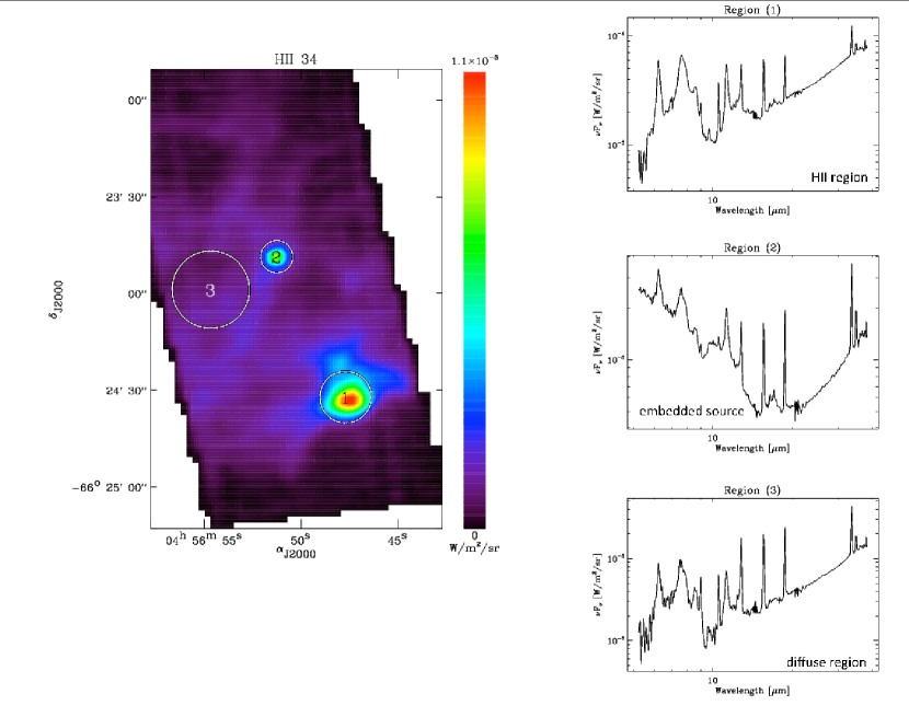
Figure 6.— Example of a spectral map of an H ii region (LHA 120-N 11; DEM L 34) and its surroundings. The map shows the integrated intensity between 6 to 9 $\mu$m for the region where there is full coverage over the entire IRS LL and SL range. The panels on the right show the extracted spectra from different regions in the map. Region 1 is centered on N11B, a compact H II region. Its IRS spectrum shows nebular line and PAH emission on a steeply rising IR continuum. Region 2 is centered on an embedded cluster which shows a strong stellar continuum together with an IR excess due to the surrounding dust. Region 3 represents a more diffuse region and it exhibits very prominent nebular lines in its IRS spectrum. (Hony et al. in prep.)

The first delivery took place on 1 August, 2009, and included the reduced data of all SAGE-Spec IRS staring mode observations, along with a first batch of MIPS SED point source observations (Woods et al., 2010). The second delivery in March 2010 contains the reduced spectral data cubes for the extended regions observed with MIPS SED and IRS (both SAGE-Spec and archival data) and the reduced archival IRS staring mode spectroscopy from Cycles 1–3 (Woods et al., 2010). Two more deliveries are planned at $\sim$6 month intervals, encompassing archival data from Cycles 4 and 5, and the enhanced data products.

4. First results

Here, we list some first scientific results of the SAGE-Spec collaboration, in the context of both program aims: Following the life cycle of gas and dust (Sect. 4.1) and the classification of point sources (Sect. 4.2).

4.1. Life cycle of gas and dust

4.1.1 Evolved stars

Carbon-rich post-AGB stars

Four carbon-rich post-AGB objects in the combined SAGE-Spec and archival samples can easily be identified by their spectral characteristics: they have strong PAH emission and exhibit the 30 $\mu$m feature generally attributed to MgS grains. In addition, the dust temperature is clearly low compared to that in carbon-stars still on the AGB as judged from the shape of the continuum. These objects most likely have left the AGB within the last few hundred years and are evolving to become planetary nebulae. The IRS spectra of the four objects along with the available photometry in the literature are presented in Figure 7. Three of the objects are SAGE-Spec targets and selected as likely post-AGB candidates, while object NGC 1978 WBT 2665 was part of the sample of PID 3591 (Tab. 5), and selected on its infrared colors using the classification by Egan et al. (2001).

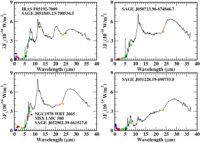
Figure 7.— IRS spectra of the four post-AGB candidate objects are given all on the same scale for direct comparison. In each panel the available photometry from the literature are also plotted: green for the SAGE-LMC IRAC photometry, orange for SAGE-LMC MIPS-24 photometry, red for 2MASS photometry (Skrutskie et al., 2006; Cohen et al., 2003), maroon for MSX (from the reject catalog for NGC 1978 WBT 2665; Price et al., 2004), blue for the Magellanic Cloud Photometric Survey photometry (Zaritsky et al., 1997), magenta for DENIS photometry (Fouqué et al., 2000), dark green for IRAS photometry (Beichman et al., 1988), and brown/cyan for Palomar Sky Survey photometry (Monet et al., 2003). No scaling has been applied to any of the data values.

IRAS F05192$-$7009 shows a strong 21 $\mu$m feature, so far only observed in post-AGB objects in our Galaxy (see for example Hrivnak et al., 2009, and references therein), thus representing the first extragalactic detection of this feature. In the other three objects it is weak or absent. For object SAGE1C J051228.18$-$690755.7 the data around the position of the feature possibly contain an artefact, so it is possible that there is a 21 $\mu$m feature present, but if so it is quite weak and it seems more likely that the feature is absent. Preliminary dust radiative transfer modeling for IRAS 05192$-$7009 shows that that the 21 $\mu$m and 30 $\mu$m feature shapes are the same as those observed in Galactic objects, and suggests that the bulk of the dust in the circumstellar shell is hotter than that found for the Galactic 21 $\mu$m sources. The models indicate that the dust shell for IRAS 05192$-$7009 is somewhat more massive than those of a number of the well studied Galactic 21 $\mu$m objects such as IRAS 07134$+$1005 and IRAS 22272$+$5435. The same may be the case for all four objects which would then suggest that they have left the AGB more recently than most of or all of the Galactic 21 $\mu$m objects.

Compared to Galactic objects of this type, the LMC sources show very strong PAH emission features including the rarely seen 6.9 $\mu$m feature. Comparison of the IRAC colors of these objects to the simulated IRAC/MIPS colors of Galactic 21 $\mu$m objects with good quality ISO SWS data indicates that the [3.6] $-$ [8.0] colors for the LMC objects are larger than those for the Galactic objects, which may be due to some combination of being less evolved off the AGB and having the strong PAH features. All of these objects have a well defined position in a K $-$ [8.0] vs. K $-$ [24] color-color diagram which suggests that further candidate post-AGB objects can be identified from the SAGE-LMC data.

RV Tauri stars

A specific sub-class of post-AGB stars is formed by the RV Tauri stars. These are pulsating stars which occupy the high-luminosity tail of the population II Cepheids. Their light curves are characterized by a succession of deep and shallow minima. Many objects also show significant cycle-to-cycle variability.

One of the more remarkable properties of RV Tauri stars is that the observed chemical pattern in the photospheres of many Galactic RV Tauri stars is the result of a chemical rather than a nucleosynthetic process: The photospheres are found to be deficient in refractory elements (like Fe and Ca and the s-process elements), while the non-refractory elements are not (or much less) affected (Giridhar et al., 2005; Maas et al., 2005, and references therein). The photospheric patterns can be understood by a process in which gas-dust separation is followed by re-accretion of only the gas, which is poor in refractory elements. This process has likely only taken place in systems which are surrounded by stable dusty disks (Waters et al., 1992), which RV Tauri stars are known to possess (Van Winckel, 2003).

These dusty disks around evolved objects are ideal environments to foster strong grain processing and in a Spitzer survey of 21 Galactic sources Gielen et al. (2008) showed that very high crystallinity prevails, and is dominated by magnesium-rich end members of olivine and pyroxene silicates. RV Tauri stars in the LMC were found by the microlensing survey MACHO (Alcock et al., 1998) and high resolution optical spectroscopy revealed that depletion of refractory elements is also observed in their photospheres (Reyniers & van Winckel, 2007).

Using SAGE-Spec data, we showed that also in the LMC, the RV Tauri stars have stable disks, rather than dusty outflows (Gielen et al., 2009) and the close connection between photospheric depletion and the stable dusty environment is illustrated in Fig. 8.

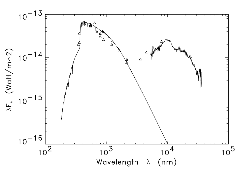
Figure 8.— The de-reddened SED of RV Tauri star MACHO 82.8405.15 (Gielen et al., 2009). Triangles are broad-band fluxes. The full line is the associated Kurucz stellar atmosphere model. The SAGE-Spec infrared spectrum is also shown. Thermal emission from amorphous silicates dominates the spectrum but substructure in the 10 $\mu$m profile as well as the presence of smaller features at longer wavelengths indicate the presence of crystalline silicates (Gielen et al., 2009). This object shows a clear correlation between abundance pattern (Reyniers & van Winckel, 2007) and condensation temperature of species, consistent with re-accretion.

4.1.2 Interstellar medium

The integrated spectrum of SAGE-Spec diffuse region #1, hereafter SSDR 1, which is also known as CO cloud 154 from the NANTEN CO survey (Fukui et al., 2008), or LMC N J0531-6830, with a mass (estimated from the CO) of $1.0\times 10^{6}$ $M_{\odot}$ (Fukui et al., 2008), is shown in Figure 5. The spectrum is dominated by PAH features at 5–15 $\mu$m and a continuum from small grains at longer wavelengths, while big grains dominate the emission longward of $\sim$80 $\mu$m. In order to extract some physical properties of the PAHs and ionic lines in the spectral cube, the spectrum was fitted using an adapted version of PAHFIT (Smith et al., 2007b) that handles both the IRS (5–40 $\mu$m) and MIPS SED (70–90 $\mu$m) spectra. To extract abundances of the PAHs and grains populations responsible for the MIR and FIR continuum emission, we used an empirical dust model, DUSTEM (see Bernard et al., 2008, for a description) which is based on the emission model of Désert et al. (1990). We fit the integrated spectrum with the DUSTEM model allowing the radiation field intensity ($X_{\mathrm{ISRF}}$), the abundance of the 3 dust components ($Y_{\mathrm{PAH}}$; Very Small Grains: $Y_{\mathrm{VSG}}$; and Big Grains: $Y_{\mathrm{BG}}$) and the intensity of the NIR continuum to vary simultaneously. The size distribution of the PAHs and BGs remain in the form of a power law as in the Solar Neighborhood (Désert et al., 1990), but we model the VSGs with a flatter size distribution to account for the flatter shape of the far-infrared continuum: $n(a)da\propto a^{\alpha}$ with $\alpha=-1$, where $a$ is the grain radius and $\alpha$ the index of the size distribution of the VSGs. The best fit is shown in Fig. 9 along with the SAGE-Spec spectrum normalized to a total dust column density of $10^{20}$ H cm^-2 as derived from the Hi and CO maps. Fig. 9 also shows the photometry points derived from integrating the SAGE-LMC IRAC and MIPS maps over the same region used to extract the spectrum.

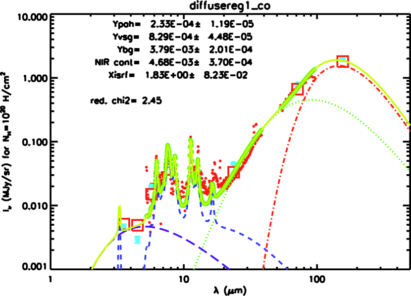
Figure 9.— Best fit derived using the DUSTEM code for the spectrum toward SSDR 1 (CO-154). The red dots show the IRS and MIPS SED SAGE-Spec spectrum integrated as discussed in the text. The blue dots show the Spitzer photometry integrated in the SAGE data for the same area. All values are normalized to a total column density of $N_{\mathrm{H}}=10^{20}$ cm^-2. The various lines show the contribution of individual dust components: red (dot-dash): Big Grains, green (dashed): Very Small Grains, blue (dashed): PAH, violet (long dash): NIR continuum. The total model spectrum is shown by the continuous yellow line. The squares show the photometry in the Spitzer bands derived from the model spectrum. The best fit values for the free parameters shown are those of Table 7.

Table 7Physical parameters derived from the DUSTEM fit compared to those obtained in Bernard et al. (2008) for cloud CO-154. The values labeled with ’H I’ are run for a grain size distribution applicable to the Solar Neighborhood, while the values labeled ’CO’ are those for case 2 as described by Bernard et al. (2008), in which the same flattened grain size distribution is used for the VSGs as in the present work.

	$Y_{\mathrm{PAH}}$	$Y_{\mathrm{VSG}}$	$Y_{\mathrm{BG}}$	NIR cont	$X_{\mathrm{ISRF}}$	$\chi^{2}/\mathrm{dof}$
	$(10^{-4})$	$(10^{-4})$	$(10^{-3})$	($10^{-4}$ MJy/sr)
SAGE-Spec	2.33	8.29	3.79	46.8	1.83	2.44
CO-154(H I)	1.78	8.25	2.85	4.99	2.59	6.61
CO-154(CO)	0.80	2.47	0.98	15.2	3.55	7.09

The DUSTEM fit results are given in Tab. 7, and shows that the dust abundances derived are somewhat in agreement with the results given in Bernard et al. (2008) for cloud CO-154, indicating that the region selected for spectral mapping is representative of the larger region mapped in the SAGE-LMC imaging survey. Note that the large value derived for the NIR continuum probably reflects that the stellar contribution was not removed from the data presented here. This does not affect the fit parameters for the PAH, VSG and BG component, as the NIR wavelength range is not used to derive the grain properties of those species.

Table 8Strengths of the major PAH features for SSDR 1, also known as NANTEN CO cloud CO-154.

Feature name	Strength	Uncertainty
	(W m-2 sr-1)	(W m-2 sr-1)
6.2 $\mu$m	1290.8	1.2
7.7 $\mu$m Complex	3374.8	5.2
8.6 $\mu$m	1525.4	1.4
11.3 $\mu$m Complex	2350.9	0.7
12.0 $\mu$m	674.3	0.9
12.6 $\mu$m Complex	945.9	0.9
13.6 $\mu$m	453.6	0.8
14.2 $\mu$m	49.0	.8
16.4 $\mu$m	171.5	.4
17 $\mu$m Complex	668.7	1.2
17.4 $\mu$m	53.1	0.4

The intensities of the major PAH features derived using PAHFIT are shown in Table 8. Figure 10 shows a comparison between the PAH strength ratios in SSDR 1 with those of other nearby galaxies (Smith et al., 2007b). The ISM for all of these extragalactic spectra contain a range of radiation fields. Although SSDR 1 is toward molecular cloud CO-154, there is clearly ionized gas in the line-of-sight, based on the presence of the $[$Ne III$]$ 15.5 and $[$Ne II$]$ 12.8 $\mu$m lines. The ratio of these lines, $[$Ne III$]$/$[$Ne II$]$=0.17, indicating low-ionization gas, is near the median of the ratios for the extragalactic lines-of-sight studied by Smith et al. (2007b). Nonetheless, we separated the high-ionization lines-of-sight in order to keep the comparison as even as possible. It is evident that the 8.6, 11.3 and 12.6 $\mu$m features are significantly stronger for SSDR 1 than the average for the sample of nearby galaxies. The relatively bright 11.3 $\mu$m feature is characteristic of the ISM in the Magellanic Clouds. The features were first detected outside H II regions in the SMC using ISO (Reach et al., 2000), for a region similar in many ways to SSDR 1 considered here; the feature ratios have been interpreted as indicating a different intrinsic set of PAH band strengths in the SMC as compared to those in the Milky Way (Li & Draine, 2002).

Figure 10.— Histograms of the ratios of PAH feature strengths from a sample of nearby galaxies (Smith et al., 2007b). Each ratio is normalized to the 7.7 $\mu$m PAH complex. The solid histograms are for the 50 galaxies in the sample with [Ne III]$<$[Ne II], as observed for SSDR 1, while the dotted histograms are for the 9 others. The feature ratios for SSDR 1 (CO-154) are indicated with vertical dashed lines.

4.1.3 Young Stellar Objects

Fig. 11 shows two examples of embedded YSOs in the SAGE-Spec sample. Both spectra exhibit strong absorption at 15.2 $\mu$m attributed to the CO₂ ice bending mode. These objects also show strong silicate absorption at 10 $\mu$m, as well as emission features due to PAHs, more noticeable at 6, 8 and 11 $\mu$m. The lower spectrum also seems to show an additional broad absorption feature at 6 $\mu$m. This ice band is mainly due to the O$-$H bending mode of water ice, but it is also thought to include contributions of other minor ice species. We have analyzed in detail the CO₂ profiles of a sample of massive embedded YSOs identified in the SAGE-Spec survey and from archival data, of which the results are presented in another paper (Oliveira et al., 2009), and summarized here. We compute column densities and compare the observed profiles with laboratory profiles available in the literature. The observed profiles show a varied morphology that, when modeled with the help of lab profiles, provides clues on the ice’s admixtures and environmental properties, like temperature. We also investigate the properties of the 5$-$7 $\mu$m band. By comparing observed properties in LMC and Galactic sample it is possible to get a handle on metallicity effects on ice chemistry (Oliveira et al., 2009).

Figure 11.— Examples of IRS spectra for 2 embedded YSOs in the LMC (Oliveira et al., 2009). Both objects exhibit a red dust continuum characteristic of the early stages of YSO evolution. Both objects show the broad feature at 10 $\mu$m associated with silicate dust and PAH emission most noticeably at 6, 8 and 13 $\mu$m. Their spectra also show prominent ice signatures: CO₂ ice at 15.2 $\mu$m, and the 5 $-$ 7 $\mu$m ice complex (for the bottom object) that includes amongst others an important contribution from water ice.

4.2. The nature of point sources

4.2.1 MIPS SED point sources

Two examples of MIPS SED spectra (van Loon et al., 2010) are shown together with their IRS spectra in Figure 3. These two objects are very different, both in their appearance and in their nature: IRAS 05280$-$6910 is an OH/IR star of high luminosity (Wood et al., 1992); it is perhaps the most dust-enshrouded supergiant known to exist in the Magellanic Clouds (van Loon et al., 2005a). We might be dealing with a flattened circumstellar envelope, such as that of WOH G064 (Ohnaka et al., 2008) but in this case viewed edge-on and thus rendering the central star invisible at optical wavelengths. This picture is confirmed by the large optical depth in the silicate features in the IRS range and the absence of cold dust in the MIPS SED range. The other object, IRAS 05137$-$6914 is an ultra-compact H II region detected at radio wavelengths (Mathewson et al., 1985; Bojičić et al., 2007). It must harbor a massive young, hot star. The cold dust dominating the cocoon around this young star emits an intense far-IR continuum. The excitation and ionization conditions in the gas are traced by the fine-structure line emission of [Oi] at 63 $\mu$m and [Oiii] at 88 $\mu$m in the MIPS SED range; in the IRS range the [Siii] lines at 18 and 33 $\mu$m are very bright and PAH emission as a consequence of the erosion of small grains is seen. We present a thorough description of the nature of all SAGE-Spec MIPS SED point sources in a related study (van Loon et al., 2010).

4.2.2 A background quasar with peculiar properties

The SAGE-Spec program has also yielded IRS spectra of a number of sources that could not easily be classified based on their broad-band colors. Several of these are background sources. One such background source – SAGE 1CJ053634.78$-$722658.5 – stands out in the IRS spectrum. It has a redshifted spectrum ($z$=0.14) that exhibits extremely prominent silicate emission features at 10 and 18 $\mu$m. We have analyzed the source and discussed its nature (Hony et al., 2010). We argue that the peculiar IRS spectrum and its corresponding broad wavelength energy distribution are indicative of a quasar. We do not detect any emission from the host galaxy; neither the stellar component in the optical or near IR nor the colder ISM in the far-IR (see Fig. 12; Hony et al., 2010), and this may thus be another example of a host-less quasar (Magain et al., 2005).

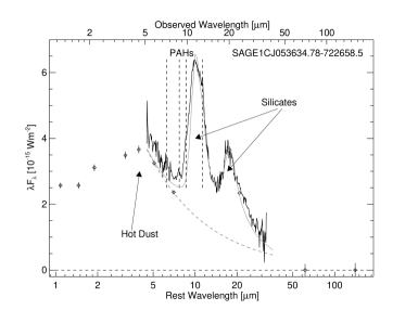
Figure 12.— Broad wavelength energy distribution of background quasar SAGE 1C J053634.78$-$722658.5 combined with the remarkable IRS spectrum of the source (Hony et al., 2010). The main contributions that can be identified are the exceptionally strong silicate emission bands at 9.7 and 18 $\mu$m and the hot continuum peaking near 4 $\mu$m. The weak PAH emission bands have been used to derive the redshift of 0.14.

5. Outlook and conclusions

The SAGE-Spec program provides useful data for understanding the life cycle of gas and dust in galaxies. The extensive dataset of IRS and MIPS SED spectroscopy, obtained within the SAGE-Spec program, complemented with archival data, sample the relevant environments and ultimately provides insights on dust mineralogy and gas properties in these environments. Feeding the results back to the original SAGE-LMC data leads to conclusions on stellar populations, and allow us to study the mineralogical dust cycle in the Large Magellanic Cloud, in combination with the global star formation rate (Whitney et al., 2008; Gruendl & Chu, 2009) and injection rate of stellar mass loss into the ISM (e.g.  Matsuura et al., 2009; Srinivasan et al., 2009). An important outcome of the SAGE-Spec program is contributing distinguishing diagnostics to classify sources in the SAGE-LMC point source catalog.

The initial results discussed in the paper include the first extragalactic detection of the 21 $\mu$m feature; the study of crystalline silicates in the disks around RV Tauri stars; the possible detection of a host-less quasar; the analysis of ices towards massive YSOs; and investigations into feature and line ratios in atomic and H II regions to probe physical conditions, such as radiation field and ionization fraction.

True to its legacy status, the SAGE-Spec team has delivered a significant fraction of its reduced data to the scientific community already, with further data deliveries planned in the near future. The unprocessed data have been available to the community in the Spitzer archive from the date of observing. We will also deliver enhanced data products, particularly spectral feature maps and source and spectral classifications in those future deliveries.

Table 3Point sources targeted with the IRS staring mode as part of the SAGE-Spec program.

Nr.	AORkey	RA (J2000)	Dec (J2000)	SAGE designation	mod.	name	AOR key	Remarks
	IRS			SSTISAGE +			MIPS SED
1	22399232	04h37m21.15s	$-$70d34m44.57s	MC J043721.15$-$703444.7	sl	NGC 1651 SAGE IRS 1		Cluster
2	22399488	04h37m27.69s	$-$67d54m34.94s	MC J043727.61$-$675435.1	sl/ll		22459648
3	22399744	04h46m27.15s	$-$68d47m46.83s	MC J044627.10$-$684747.0	sl/ll
4	22400256	04h47m18.63s	$-$69d42m20.53s	MC J044718.63$-$694220.6	sl/ll
5	24319488	04h48m37.75s	$-$69d23m36.85s	MC J044837.77$-$692337.0	sl/ll
6	24318720	04h49m34.38s	$-$69d05m49.17s	MC J044934.31$-$690549.3	sl/ll
7	22400512	04h50m40.57s	$-$68d58m18.76s	MC J045040.52$-$685819.0	sl/ll	MSX LMC 1128
8	22400768	04h51m28.58s	$-$69d55m49.92s	MC J045128.58$-$695550.1	sl/ll
9	22401024	04h51m40.63s	$-$68d47m34.82s	MC J045140.57$-$684734.6	sl/ll	IRAS 04518$-$6852
10	22401280	04h52m00.38s	$-$69d18m05.53s	MC J045200.36$-$691805.6	sl/ll
11	24315136	04h52m28.66s	$-$68d54m51.09s	MC J045228.68$-$685451.3	sl/ll
12	22401792	04h52m32.49s	$-$67d02m59.30s	MC J045232.54$-$670259.2	sl	KDM 764		Cluster
13	22402048	04h53m09.54s	$-$68d17m10.11s	MC J045309.39$-$681710.8	sl
14	24317952	04h53m11.03s	$-$67d03m55.96s	1C J045311.04$-$670355.6	sl/ll	IRAS F04532$-$6709
15	22402304	04h53m28.71s	$-$66d03m34.76s	MC J045328.70$-$660334.4	sl
16	22402560	04h53m30.86s	$-$69d17m49.85s	MC J045330.88$-$691749.7	sl	GV 60
17	22402560	04h53m30.86s	$-$69d17m49.85s		ll	LH$\alpha$ 120$-$N 82	22457088
18	24319232	04h53m44.28s	$-$66d11m45.76s	MC J045344.24$-$661146.0	sl/ll
19	22403072	04h54m22.88s	$-$70d26m56.64s	MC J045422.82$-$702657.0	sl			Cluster
20	22403328	04h55m26.76s	$-$68d25m07.93s	MC J045526.69$-$682508.4	sl/ll
21	24318976	04h55m34.06s	$-$65d57m00.92s	MC J045534.07$-$655701.3	sl/ll
22	22404096	04h56m23.27s	$-$69d27m48.05s	MC J045623.21$-$692749.0	sl/ll
23	22404864	04h58m55.03s	$-$69d11m18.21s	MC J045855.02$-$691118.7	sl	KDM 1238
24	22405120	04h58m55.29s	$-$68d50m36.13s		sl
25	22405632	05h00m32.59s	$-$66d21m12.60s	MC J050032.61$-$662113.0	sl/ll
26	22405888	05h00m34.69s	$-$70d52m00.34s	MC J050034.61$-$705200.4	sl/ll	RP 1631
27	22406144	05h02m21.52s	$-$66d06m37.98s	MC J050221.46$-$660638.3	sl/ll	MSX LMC 1271		Cluster
28	22406400	05h02m24.21s	$-$66d06m37.46s	MC J050224.17$-$660637.4	sl/ll	NGC 1805 SAGE IRS 1		Cluster
29	22406656	05h03m04.98s	$-$68d40m24.90s	MC J050304.95$-$684024.7	sl/ll	HV 2281
30	22406912	05h03m16.59s	$-$65d49m44.79s	MC J050316.60$-$654945.1	sl	KDM 1656
31	22407168	05h03m36.89s	$-$68d33m38.71s	MC J050336.92$-$683338.5	sl	KDM 1691
32	22407424	05h03m42.54s	$-$67d59m18.83s	MC J050342.57$-$675919.2	sl	LMC$-$BM 11$-$19
33	22407680	05h03m53.50s	$-$70d27m47.53s	MC J050353.40$-$702747.6	sl	LMC$-$BM 12$-$14
34	24317696	05h03m54.60s	$-$67d18m47.69s	MC J050354.55$-$671848.7	sl/ll
35	22407936	05h04m07.38s	$-$66d26m42.71s	MC J050407.42$-$662643.0	sl	NGC 1818 WBT 5		Cluster
36	22408192	05h04m07.73s	$-$66d25m05.48s	MC J050407.72$-$662505.9	sl	NGC 1818 WBT 64		Cluster
37	22408448	05h04m11.09s	$-$66d26m16.70s	MC J050411.04$-$662616.8	sl	NGC 1818 WBT 3		Cluster
38	22408704	05h04m28.91s	$-$67d41m23.43s	MC J050428.91$-$674123.9	sl/ll	MSX LMC 61
39	22408960	05h04m34.17s	$-$67d52m21.05s	MC J050434.20$-$675221.8	sl/ll	RP 1878
40	24317440	05h04m51.71s	$-$66d38m07.41s	MC J050451.70$-$663807.5	sl/ll	IRAS 05047$-$6642
41	24314880	05h05m03.22s	$-$69d24m26.51s	MC J050503.21$-$692426.5	sl			Cluster
42	22409216	05h05m17.19s	$-$69d21m57.12s	MC J050517.08$-$692157.0	sl/ll
43	22409472	05h05m55.74s	$-$67d22m09.24s	MC J050555.66$-$672210.0	sl	LMC$-$BM 13$-$2
44	22409728	05h05m58.26s	$-$68d09m23.79s	MC J050558.23$-$680923.6	sl/ll
45	22409984	05h06m07.51s	$-$71d41m48.12s	MC J050607.50$-$714148.4	sl
46	22410240	05h06m12.61s	$-$64d55m37.23s	MC J050612.59$-$645537.5	sl	KDM 1961		Cluster
47	22410496	05h06m18.95s	$-$64d56m10.88s	MC J050618.98$-$645610.2	sl	KDM 1966		Cluster
48	22410752	05h06m20.13s	$-$64d54m58.01s	MC J050620.12$-$645458.6	sl			Cluster
49	22411008	05h06m29.62s	$-$68d55m34.54s	MC J050629.61$-$685534.9	sl
50	22411264	05h06m39.24s	$-$68d22m09.32s	MC J050639.14$-$682209.3	sl/ll
51	22411520	05h07m09.47s	$-$68d58m50.18s	2C J050709.45$-$685849.3	sl/ll	SHV 0507252$-$690238		Cluster
52	24317184	05h07m14.00s	$-$67d48m46.46s	MC J050713.90$-$674846.7	sl/ll
53	22411776	05h07m53.01s	$-$68d12m46.38s	MC J050752.93$-$681246.5	sl/ll
54	22412032	05h07m59.36s	$-$68d39m25.71s	MC J050759.35$-$683925.8	sl/ll
55	22412288	05h08m26.27s	$-$68d31m15.01s	MC J050826.35$-$683115.1	sl/ll
56	22412544	05h08m30.62s	$-$69d22m37.39s	MC J050830.51$-$692237.4	sl/ll
57	22412800	05h08m36.42s	$-$69d43m15.11s	MC J050836.39$-$694315.7	sl	KDM 2187
58	22413056	05h09m26.44s	$-$69d06m56.99s	MC J050926.57$-$690656.3	sl	BMB$-$BW 180		Cluster
59	22413312	05h09m29.54s	$-$69d07m50.90s	MC J050929.53$-$690750.3	sl	NGC 1856 SAGE IRS 1		Cluster
60	22414080	05h10m28.38s	$-$68d44m31.44s	1C J051028.32$-$684431.4	sl/ll			Cluster
61	22414336	05h10m59.06s	$-$68d56m13.82s	MC J051059.07$-$685613.7	sl/ll
62	22414592	05h12m09.19s	$-$71d06m49.52s	MC J051209.02$-$710649.7	sl/ll	MSX LMC 209
63	22414848	05h12m13.57s	$-$68d39m22.47s	MC J051213.54$-$683922.8	sl
64	24316928	05h12m28.17s	$-$69d07m56.15s	MC J051228.19$-$690755.8	sl/ll
65	22415104	05h13m01.80s	$-$69d33m51.21s	MC J051301.75$-$693351.0	sl/ll	IRAS 05133$-$6937
66	22415360	05h13m06.43s	$-$69d09m46.53s	1C J051306.40$-$690946.3	sl/ll	OGLE J051306.52$-$690946.4
67	22415616	05h13m39.87s	$-$66d38m52.70s	MC J051339.94$-$663852.5	sl
68	22416128	05h13m41.42s	$-$65d28m27.91s	MC J051341.40$-$652828.2	sl	NGC 1866 Robb B136		Cluster
69	22416384	05h13m42.83s	$-$67d24m10.44s	MC J051342.63$-$672409.9	sl/ll	BSDL 923
70	24316672	05h13m47.79s	$-$69d35m05.06s	MC J051347.72$-$693505.2	sl/ll
71	22416640	05h13m48.33s	$-$67d05m26.87s	MC J051348.38$-$670527.0	sl/ll
72	22416896	05h14m12.32s	$-$68d50m58.29s	MC J051412.33$-$685058.0	sl
73	22417152	05h14m18.15s	$-$69d12m35.06s	MC J051418.09$-$691234.9	sl/ll	HV 915
74	24316416	05h14m49.41s	$-$67d12m22.24s	MC J051449.43$-$671221.4	sl/ll
75	22417408	05h14m53.12s	$-$69d17m23.70s	MC J051453.10$-$691723.5	sl/ll
76	22417664	05h15m26.47s	$-$67d51m26.91s	MC J051526.44$-$675126.9	sl
77	22417920	05h16m12.52s	$-$70d49m30.18s	MC J051612.42$-$704930.3	sl
78	22418176	05h16m18.69s	$-$71d53m59.21s	MC J051618.69$-$715359.0	sl/ll	IRAS 05170$-$7156
79	22418688	05h17m47.16s	$-$68d18m42.64s	MC J051747.18$-$681842.6	sl
80	22418944	05h18m03.28s	$-$68d49m50.29s	1C J051803.23$-$684950.7	sl/ll
81	22419200	05h18m07.94s	$-$71d51m53.66s	MC J051807.93$-$715153.7	sl	KDM 3196
82	22419456	05h18m11.05s	$-$67d26m48.92s	MC J051811.08$-$672648.5	sl/ll	HV 5715
83	22419712	05h18m32.63s	$-$69d25m25.59s	MC J051832.64$-$692525.5	sl			Cluster
84	24314624	05h18m45.27s	$-$70d05m34.70s	MC J051845.23$-$700534.5	sl/ll	IRAS F05192$-$7008
85	27037952	05h18m45.46s	$-$69d03m21.65s	MC J051845.47$-$690321.8	sl/ll	HV 2444
86	22419968	05h19m08.52s	$-$69d23m14.44s	MC J051908.46$-$692314.3	sl
87	22420224	05h19m10.63s	$-$69d33m46.51s	MC J051910.49$-$693345.3	sl	2MASS J05191049$-$6933453
88	22420480	05h19m44.87s	$-$69d29m59.84s	MC J051944.81$-$692959.4	sl	2MASS J05194483$-$6929594
89	22420736	05h20m14.31s	$-$70d29m31.33s	MC J052014.24$-$702931.0	sl
90	22420992	05h20m23.97s	$-$69d54m23.08s	MC J052023.97$-$695423.2	sl/ll
91	22421248	05h20m51.86s	$-$69d34m08.04s	MC J052051.83$-$693407.6	sl
92	22421504	05h20m52.44s	$-$70d09m35.60s	MC J052052.42$-$700935.5	sl/ll	LH$\alpha$ 120$-$N 125
93	22421760	05h21m01.71s	$-$69d14m17.07s	MC J052101.66$-$691417.5	sl/ll
94	22422016	05h21m47.99s	$-$70d09m57.22s	MC J052147.95$-$700957.0	sl/ll	HV 942
95	22422272	05h21m49.40s	$-$70d04m35.26s	MC J052149.11$-$700434.2	sl/ll	MACHO 78.6698.38
96	22422528	05h22m06.91s	$-$71d50m17.89s	MC J052206.92$-$715017.7	sl/ll
97	22422784	05h22m22.98s	$-$68d41m00.72s	MC J052222.95$-$684101.2	sl/ll		22457856
98	22423040	05h22m42.01s	$-$69d15m26.04s	MC J052241.93$-$691526.2	sl/ll	OGLE 052242.09$-$691526.2
99	22423552	05h22m54.96s	$-$69d36m52.34s	MC J052254.97$-$693651.7	sl	SHV 0523185$-$693932
100	22423808	05h23m31.25s	$-$69d04m04.56s	MC J052331.11$-$690404.6	sl/ll	LH$\alpha$ 120$-$N 136
101	22424320	05h23m51.14s	$-$68d07m12.37s	MC J052351.13$-$680712.2	sl/ll	IRAS 05240$-$6809
102	22424576	05h23m53.95s	$-$71d34m43.97s	MC J052353.92$-$713443.9	sl/ll	IRAS 05246$-$7137	22458112
103	22424832	05h24m05.25s	$-$68d18m01.99s	MC J052405.31$-$681802.5	sl/ll
104	22425088	05h24m13.30s	$-$68d29m58.98s	MC J052413.36$-$682958.8	sl/ll	MSX LMC 464
105	22425344	05h24m45.36s	$-$69d16m05.53s	MC J052445.38$-$691605.3	sl/ll	OGLE J052445.53$-$691605.6
106	22425600	05h24m57.86s	$-$67d24m58.43s	MC J052457.85$-$672458.3	sl/ll	LH$\alpha$ 120$-$S 33
107	24314368	05h25m19.52s	$-$70d54m09.84s	MC J052519.48$-$705410.0	sl/ll	HV 5829
108	24319744	05h25m46.52s	$-$66d14m11.30s	MC J052546.51$-$661411.5	sl/ll
109	24315904	05h26m13.35s	$-$68d47m15.24s	MC J052613.39$-$684715.0	sl/ll
110	22426112	05h26m20.15s	$-$69d39m02.59s	MC J052620.10$-$693902.1	sl	OGLE J052620.25$-$693902.4
111	27038208	05h26m27.19s	$-$66d42m58.66s	MC J052627.23$-$664258.7	sl/ll	HV 2522
112	22426368	05h26m37.58s	$-$70d29m07.18s	MC J052637.81$-$702906.7	sl	RP 589
113	22426624	05h27m07.14s	$-$70d20m02.12s	MC J052707.10$-$702001.9	sl/ll
114	22426880	05h27m23.24s	$-$71d24m25.41s	MC J052723.14$-$712426.3	sl/ll		22458624
115	22427136	05h27m35.64s	$-$69d08m56.22s	MC J052735.63$-$690856.3	sl	LH$\alpha$ 120$-$N 145		Cluster
116	22427392	05h27m38.76s	$-$69d28m45.57s	MC J052738.58$-$692843.9	sl/ll	HV 2551
117	22427648	05h27m39.62s	$-$69d09m01.57s	MC J052739.63$-$690901.4	sl/ll	W61 11$-$16		Cluster
118	22427904	05h27m47.60s	$-$71d48m52.75s	MC J052747.62$-$714852.8	sl/ll
119	22428160	05h28m05.91s	$-$70d07m54.03s	MC J052805.91$-$700753.4	sl/ll	SHV 0528350$-$701014
120	22428416	05h28m25.86s	$-$69d46m47.45s	MC J052825.81$-$694647.3	sl	OGLE J052825.96$-$694647.4
121	27084288	05h29m24.61s	$-$69d55m14.19s	1C J052924.59$-$695513.4	sl/ll	IRAS 05298$-$6957	22448896
122	22428672	05h29m54.80s	$-$69d04m15.73s	MC J052954.73$-$690415.7	sl/ll	HV 5879
123	22428928	05h30m04.67s	$-$68d47m29.08s	MC J053004.56$-$684728.8	sl/ll	SP77 46$-$50
124	22429184	05h30m27.56s	$-$69d03m59.04s	MC J053027.49$-$690358.3	sl	SHV 0530472$-$690607
125	22429440	05h30m44.72s	$-$71d42m59.62s	MC J053044.71$-$714259.4	sl/ll	IRAS 05315$-$7145
126	22429696	05h30m45.03s	$-$68d21m29.11s	1C J053044.97$-$682129.1	sl/ll	KDM 4554
127	22429952	05h30m46.74s	$-$67d16m56.92s	MC J053046.81$-$671657.2	sl	NGC 2004 Robb B45		Cluster
128	22430208	05h30m48.40s	$-$67d16m45.88s	MC J053048.42$-$671645.8	sl/ll	NGC 2004 Wes 18$-$13		Cluster
129	22430464	05h30m52.25s	$-$67d17m34.22s	MC J053052.28$-$671734.4	sl/ll	NGC 2004 Wes 6$-$14		Cluster
130	22430720	05h31m28.43s	$-$70d10m27.65s	MC J053128.44$-$701027.1	sl/ll
131	22430976	05h31m51.01s	$-$69d11m46.56s	MC J053150.98$-$691146.4	sl/ll	MACHO 82.8405.15
132	22431232	05h31m58.96s	$-$72d44m36.35s	MC J053158.92$-$724436.0	sl	KDM 4665
133	22431488	05h32m06.64s	$-$70d10m25.34s	MC J053206.70$-$701024.8	sl			Cluster
134	22431744	05h32m18.66s	$-$67d31m46.16s	MC J053218.64$-$673145.9	sl			Cluster
135	22432000	05h32m19.31s	$-$67d31m20.34s	MC J053219.33$-$673120.5	sl/ll	NGC 2011 SAGE IRS 1		Cluster
136	22432256	05h32m26.52s	$-$73d10m06.99s	MC J053226.51$-$731006.8	sl	KDM 4718
137	24318208	05h32m39.71s	$-$69d30m49.25s	MC J053239.68$-$693049.4	sl/ll	RP 774
138	22432768	05h32m53.35s	$-$66d07m27.17s	MC J053253.36$-$660727.8	sl/ll
139	22433024	05h32m54.98s	$-$67d36m47.10s	MC J053254.99$-$673647.2	sl	KDM 4774
140	24314112	05h33m06.86s	$-$70d30m34.22s	MC J053306.86$-$703033.9	sl/ll	MSX LMC 736
141	22433280	05h33m18.61s	$-$66d00m39.91s	MC J053318.58$-$660040.2	sl/ll
142	22433536	05h33m43.18s	$-$70d59m21.16s	MC J053343.27$-$705921.1	sl			Cluster
143	22433792	05h33m44.00s	$-$70d59m01.14s	MC J053343.98$-$705901.9	sl			Cluster
144	22434048	05h33m46.97s	$-$68d36m44.08s	MC J053346.97$-$683644.2	sl/ll	LH$\alpha$ 120$-$N 151
145	22434304	05h34m41.46s	$-$69d26m30.74s	MC J053441.40$-$692630.6	sl/ll
146	22434560	05h34m44.20s	$-$67d37m50.82s	MC J053444.17$-$673750.1	sl/ll	SHP LMC 256
147	22434816	05h35m19.01s	$-$67d02m19.50s	MC J053518.91$-$670219.5	sl/ll	HV 2700
148	22435072	05h35m48.02s	$-$70d31m46.92s	MC J053548.07$-$703146.6	sl
149	22435328	05h36m02.42s	$-$67d45m17.41s	MC J053602.36$-$674517.3	sl/ll
150	24315648	05h36m32.48s	$-$70d17m38.81s	MC J053632.56$-$701738.4	sl/ll	IRAS 05370$-$7019
151	22435584	05h36m34.82s	$-$72d26m58.67s	MC J053634.77$-$722658.6	sl/ll
152	22436096	05h36m55.68s	$-$68d11m24.31s	MC J053655.60$-$681124.6	sl
153	22436352	05h37m10.12s	$-$71d23m14.06s	MC J053710.26$-$712314.3	sl	RP 493
154	22436608	05h37m30.63s	$-$67d40m41.19s	MC J053730.59$-$674041.6	sl/ll
155	22437120	05h38m23.66s	$-$66d09m00.91s	MC J053823.58$-$660900.3	sl	KDM 5345
156	22437376	05h39m29.94s	$-$69d57m56.27s	1C J053929.96$-$695755.6	sl/ll	OGLE J053930.16$-$695755.8
157	22437632	05h39m33.17s	$-$71d21m55.45s	1C J053932.66$-$712154.7	sl/ll	HV 12631
158	22437888	05h39m42.37s	$-$71d10m45.03s	MC J053942.45$-$711044.5	sl/ll
159	22438144	05h39m45.46s	$-$66d58m09.75s	MC J053945.40$-$665809.4	sl	WOH G 449
160	22438400	05h39m49.22s	$-$69d37m47.03s	MC J053949.23$-$693747.0	sl/ll
161	22438912	05h40m00.47s	$-$69d42m14.85s	MC J054000.52$-$694214.6	sl	MACHO 81.9728.14
162	22439424	05h40m14.78s	$-$69d28m49.33s	MC J054014.83$-$692849.1	sl/ll	MSX LMC 949
163	22439680	05h40m33.51s	$-$70d32m41.06s	MC J054033.54$-$703240.8	sl/ll	RP 85	22460160
164	22439936	05h40m59.28s	$-$70d44m02.82s	MC J054059.31$-$704402.5	sl/ll
165	22440192	05h41m02.04s	$-$70d43m10.55s	1C J054101.91$-$704311.0	sl/ll	MSX LMC 947
166	22440448	05h41m14.58s	$-$71d32m36.01s	MC J054114.56$-$713236.0	sl/ll
167	22440704	05h41m20.69s	$-$69d04m44.46s	1C J054120.72$-$690443.5	sl/ll	IRAS 05416$-$6906
168	24315392	05h41m25.08s	$-$71d15m32.74s	MC J054125.09$-$711532.6	sl/ll	IRAS 05421$-$7116
169	22440960	05h41m57.43s	$-$69d12m18.61s	MC J054157.40$-$691218.1	sl/ll	W61 6$-$24
170	22441472	05h42m03.91s	$-$69d13m07.64s	1C J054203.85$-$691307.1	sl/ll	NGC 2100 Robb 4		Cluster
171	22441728	05h42m06.76s	$-$69d12m31.35s	MC J054206.76$-$691231.1	sl/ll	2MASS J05420676$-$6912312		Cluster
172	22441984	05h42m09.98s	$-$69d13m28.76s	MC J054209.95$-$691328.7	sl/ll	W61 6$-$57		Cluster
173	22442240	05h42m30.51s	$-$69d48m57.47s	MC J054230.55$-$694857.3	sl	WOH G 494
174	22442496	05h42m33.35s	$-$70d29m24.18s	MC J054233.17$-$702924.1	sl/ll	LM 2$-$42
175	22443008	05h42m36.63s	$-$70d09m32.50s	MC J054236.65$-$700932.0	sl/ll	LH$\alpha$ 120$-$N 178
176	22443264	05h42m54.62s	$-$70d08m07.74s	MC J054254.38$-$700807.4	sl
177	22443520	05h43m10.87s	$-$67d27m28.42s	MC J054310.86$-$672728.0	sl/ll	IRAS F05432$-$6728
178	22443776	05h43m14.23s	$-$70d38m35.12s	MC J054314.12$-$703835.1	sl
179	22444032	05h43m28.77s	$-$69d42m43.88s	MC J054328.84$-$694243.7	sl	KDM 5841
180	22444288	05h44m06.10s	$-$68d37m53.68s	MC J054406.01$-$683753.6	sl/ll
181	22444544	05h44m37.92s	$-$67d36m58.17s	MC J054437.87$-$673657.7	sl/ll
182	22444800	05h44m40.08s	$-$69d11m49.11s	MC J054440.11$-$691149.0	sl/ll
183	22445056	05h44m50.23s	$-$69d23m04.72s	MC J054450.23$-$692304.2	sl/ll	IRAS 05452$-$6924
184	22445312	05h45m24.23s	$-$68d30m41.61s	MC J054524.23$-$683041.4	sl/ll
185	22445824	05h45m46.35s	$-$67d32m39.16s	MC J054546.32$-$673239.4	sl/ll
186	22446080	05h47m04.62s	$-$69d27m34.24s	MC J054704.54$-$692733.9	sl/ll	LH$\alpha$ 120$-$N 170
187	22446336	05h47m45.80s	$-$68d07m34.26s	MC J054745.79$-$680734.1	sl/ll
188	22446592	05h47m57.25s	$-$68d14m56.90s	MC J054757.37$-$681457.0	sl	KDM 6247
189	22446848	05h48m16.84s	$-$71d28m39.64s	MC J054816.79$-$712839.3	sl	NGC 2121 LE 6		Cluster
190	22447104	05h49m00.12s	$-$70d33m22.51s	MC J054900.01$-$703322.5	sl/ll	IRAS 05495$-$7034
191	22447360	05h50m36.62s	$-$68d28m52.27s	MC J055036.69$-$682852.4	sl	KDM 6486
192	27038464	05h51m22.58s	$-$69d53m51.05s	MC J055122.52$-$695351.4	sl/ll	HV 2862
193	22447616	05h51m43.25s	$-$68d45m42.79s	MC J055143.27$-$684543.0	sl/ll
194	22447872	05h52m51.07s	$-$69d28m39.09s	MC J055251.05$-$692839.6	sl	PMP 337		Cluster
195	22448128	05h52m52.51s	$-$69d30m35.54s	MC J055252.50$-$693035.6	sl	PMP 133		Cluster
196	27084032	05h53m12.04s	$-$70d15m22.71s	MC J055311.98$-$701522.5	sl/ll	IRAS 05537$-$7015
197	22448384	06h00m53.60s	$-$68d00m39.08s	MC J060053.62$-$680038.8	sl

Table 4Point sources targeted with the IRS staring mode as part of the SAGE-Spec program, part II.

Nr.	$J$	$H$	$K$	[3.6]	[4.5]	[5.8]	[8.0]	[24]
1	12.41	11.49	11.19	10.91	10.81	10.69	10.49	9.64
2	16.02	15.16	14.45	14.02	13.52	13.09	10.12	7.03
3	15.02	13.28	11.72	9.86	8.97	8.55	8.12	7.33
4	10.10	9.27	9.00	8.87	9.05	8.87	8.75	7.55
5	$\cdots$	$\cdots$	12.92	10.36	9.48	8.68	7.85	4.86
6	12.18	11.78	11.24	10.07	9.60	9.21	8.56	7.21
7	13.22	11.56	10.37	9.37	8.94	8.57	8.14	7.62
8	15.05	13.78	12.94	11.12	10.61	10.04	9.19	7.23
9	$\cdots$	$\cdots$	$\cdots$	12.61	10.38	8.63	7.02	4.20
10	$\cdots$	16.89	15.83	13.65	12.35	11.11	9.70	3.12
11	$\cdots$	$\cdots$	$\cdots$	12.36	11.18	10.07	8.61	3.84
12	12.02	10.79	10.03	9.22	9.36	9.35	8.80	8.46
13	12.26	11.31	10.99	10.74	10.77	10.59	10.49	10.16
14	16.94	16.14	14.89	12.85	11.63	10.25	8.95	3.22
15	12.54	11.30	10.43	9.40	9.26	8.96	8.46	8.17
16	9.32	8.46	8.06	7.50	7.46	7.13	6.51	$\cdots$
17	$\cdots$	$\cdots$	$\cdots$	$\cdots$	$\cdots$	$\cdots$	$\cdots$	1.86
18	$\cdots$	$\cdots$	$\cdots$	11.55	9.71	8.18	7.56	4.22
19	9.19	8.67	8.60	8.92	8.54	8.47	8.44	8.41
20	16.79	15.27	13.77	11.76	11.03	10.07	8.66	2.40
21	17.32	16.32	14.38	11.11	9.92	8.89	7.68	4.35
22	12.42	11.74	11.43	10.53	10.42	10.07	9.49	7.19
23	12.40	11.23	10.68	10.02	10.07	9.97	9.56	9.51
24	$\cdots$	$\cdots$	$\cdots$	$\cdots$	$\cdots$	$\cdots$	$\cdots$	$\cdots$
25	17.65	16.72	15.71	13.97	13.14	11.99	10.52	7.04
26	$\cdots$	15.22	$\cdots$	10.51	9.67	9.00	8.34	6.32
27	8.94	8.10	7.73	7.56	7.67	7.34	6.88	4.89
28	$\cdots$	$\cdots$	$\cdots$	11.08	10.22	9.52	8.56	6.29
29	13.75	13.41	13.09	11.53	10.59	9.73	8.59	6.52
30	11.59	10.43	9.78	9.06	9.09	8.90	8.26	8.23
31	11.49	10.31	9.69	8.97	9.08	8.93	8.44	7.85
32	12.05	11.13	10.83	10.54	10.73	10.56	10.37	10.00
33	11.67	10.55	9.95	9.21	9.30	9.21	8.74	8.33
34	16.15	14.13	12.35	10.15	9.26	8.51	7.49	3.67
35	10.65	9.87	9.63	9.45	9.65	9.54	9.50	9.39
36	12.41	11.34	10.85	10.33	10.15	9.88	9.55	8.97
37	10.31	9.51	9.26	9.07	9.25	9.11	8.99	8.41
38	10.93	9.97	9.39	9.21	8.98	8.73	7.99	5.62
39	16.39	15.27	14.33	12.53	11.77	11.05	10.14	7.50
40	13.98	13.17	12.22	10.49	9.87	9.06	7.94	3.60
41	12.44	11.35	$\cdots$	10.13	10.20	10.10	9.65	9.56
42	$\cdots$	$\cdots$	$\cdots$	14.28	13.18	11.96	10.65	6.54
43	14.13	12.58	11.71	10.18	9.83	9.43	9.01	8.49
44	14.68	13.89	13.47	13.18	12.55	12.04	10.82	7.08
45	12.64	11.39	10.49	9.71	9.27	8.92	8.67	8.33
46	12.96	11.97	11.59	10.93	10.91	10.75	10.61	10.42
47	12.67	11.68	11.29	10.88	10.97	10.80	10.51	10.21
48	11.86	10.71	10.09	9.33	9.40	9.33	8.75	8.65
49	12.88	11.60	11.01	10.24	10.40	10.53	9.85	9.74
50	13.10	13.09	13.10	13.06	13.04	12.91	12.58	6.57
51	12.63	11.15	10.06	8.55	8.35	8.05	7.72	7.56
52	16.62	15.38	14.50	12.22	11.32	9.68	7.57	3.26
53	15.51	13.72	12.13	9.74	9.06	8.51	8.05	7.48
54	13.30	12.32	11.96	11.18	10.56	9.91	8.95	6.82
55	15.34	13.32	11.74	9.36	8.88	8.37	7.90	7.36
56	12.46	11.54	11.09	10.49	10.25	9.88	8.40	5.36
57	12.98	11.91	11.42	10.79	10.83	10.52	10.16	9.46
58	11.61	10.71	10.38	10.23	10.38	10.23	10.18	10.02
59	13.15	12.75	12.62	$\cdots$	11.89	11.41	10.59	8.39
60	15.36	13.13	11.35	9.86	8.89	8.16	7.47	6.42
61	10.81	9.85	9.53	9.12	9.18	8.92	8.58	6.83
62	13.71	13.19	12.11	10.11	9.32	8.60	7.48	4.71
63	12.28	11.33	10.97	10.68	10.65	10.49	10.05	8.03
64	15.63	15.11	14.27	12.42	11.80	10.11	8.25	3.64
65	$\cdots$	16.44	$\cdots$	15.82	13.70	10.68	7.85	3.32
66	14.16	12.30	10.89	9.13	8.47	7.93	7.45	6.83
67	12.26	11.32	10.99	10.76	10.75	10.59	10.34	9.03
68	11.41	10.50	10.23	10.00	10.17	9.99	9.93	9.73
69	12.93	12.84	12.69	13.01	12.93	12.82	12.36	5.27
70	$\cdots$	$\cdots$	15.58	$\cdots$	11.90	10.36	8.90	3.36
71	18.06	17.08	16.01	14.16	13.38	12.53	11.43	7.51
72	12.33	11.37	11.07	10.87	10.87	10.69	10.51	9.18
73	13.09	12.63	12.09	10.14	9.39	8.67	7.84	6.01
74	17.43	15.21	13.20	10.41	9.30	8.38	7.38	3.49
75	13.48	12.71	12.51	12.15	11.77	10.94	9.51	6.13
76	12.13	11.25	10.89	10.60	10.76	10.59	10.47	10.26
77	12.26	11.35	11.08	10.78	10.83	10.68	10.47	9.28
78	$\cdots$	16.21	$\cdots$	11.61	10.38	9.20	7.61	2.97
79	13.14	12.18	11.90	11.68	11.59	11.40	10.68	8.84
80	$\cdots$	$\cdots$	$\cdots$	9.38	9.20	8.69	8.32	7.85
81	11.97	10.95	10.58	10.18	10.20	10.04	9.85	9.38
82	10.36	9.43	9.06	8.80	8.92	8.63	8.46	6.93
83	12.26	11.09	10.43	9.76	9.93	9.99	9.46	9.16
84	14.66	14.22	13.99	12.70	11.53	9.43	7.16	3.41
85	13.54	13.17	12.66	10.79	10.14	9.57	8.68	6.73
86	11.78	10.65	10.05	9.54	9.66	9.60	9.06	8.53
87	11.78	10.56	9.86	9.16	9.37	9.47	8.83	7.71
88	12.54	11.62	11.28	11.05	11.09	10.92	10.72	$\cdots$
89	12.53	11.57	11.28	11.11	11.04	10.90	10.65	9.37
90	15.63	14.94	13.80	11.34	10.34	9.50	8.46	3.61
91	12.36	11.41	11.08	10.83	10.80	10.62	10.20	8.36
92	15.97	15.61	14.27	11.73	10.69	9.17	7.40	3.30
93	11.72	10.81	10.52	10.22	10.34	10.11	9.40	7.41
94	13.36	12.82	11.89	9.85	8.99	8.22	7.43	5.97
95	14.35	13.77	13.60	12.27	11.42	10.56	9.53	7.19
96	12.40	11.47	11.20	11.00	10.95	10.74	9.66	7.70
97	15.57	14.66	13.67	11.90	11.28	9.96	8.42	4.92
98	15.79	13.60	11.81	9.46	8.72	8.16	7.60	6.83
99	12.74	11.77	11.44	11.19	11.05	10.84	10.34	8.51
100	$\cdots$	$\cdots$	15.07	13.36	12.45	11.72	10.13	6.76
101	12.99	12.28	11.79	10.24	9.33	8.59	7.63	1.90
102	$\cdots$	15.59	12.98	9.78	8.65	7.73	6.83	3.29
103	15.12	13.34	11.78	9.63	9.10	8.63	8.24	7.60
104	14.24	12.51	11.06	9.11	8.26	7.44	6.41	2.43
105	12.26	10.90	9.93	9.06	8.56	8.12	7.82	7.05
106	13.92	13.28	12.51	11.00	10.44	9.98	9.35	7.65
107	14.22	13.83	13.46	10.90	10.12	9.50	8.65	6.59
108	$\cdots$	15.46	12.92	9.93	8.75	7.90	6.87	2.89
109	15.66	14.97	14.14	12.38	11.59	10.20	8.17	3.68
110	12.26	11.38	11.10	10.65	10.82	10.54	10.21	8.30
111	13.58	13.14	12.74	11.15	10.28	9.50	8.51	6.52
112	$\cdots$	$\cdots$	$\cdots$	13.53	12.59	11.73	10.71	8.03
113	$\cdots$	$\cdots$	$\cdots$	11.44	10.67	10.17	9.48	7.56
114	17.33	$\cdots$	15.91	13.85	13.45	11.02	9.15	4.07
115	15.06	14.47	12.88	9.95	8.76	7.79	6.56	4.14
116	9.33	8.52	8.22	8.03	8.18	7.98	7.79	5.88
117	9.06	8.25	7.97	7.70	7.91	7.70	7.59	7.40
118	13.48	12.75	11.77	10.07	9.39	8.89	8.12	6.04
119	12.34	10.97	9.99	8.95	8.84	8.75	8.29	6.53
120	11.84	10.83	10.40	9.89	9.93	9.77	9.36	8.90
121	$\cdots$	$\cdots$	11.38	7.47	6.67	5.99	5.08	2.19
122	9.42	8.69	8.41	8.25	8.38	8.15	7.90	6.80
123	9.80	9.03	8.77	8.58	8.80	8.58	8.40	7.42
124	12.46	11.76	11.46	10.65	10.61	10.32	10.10	9.68
125	$\cdots$	$\cdots$	$\cdots$	13.88	12.19	10.23	7.83	2.75
126	$\cdots$	12.63	11.14	9.10	8.62	7.75	7.70	7.19
127	10.76	10.01	9.77	9.65	9.82	9.69	9.69	9.31
128	9.98	9.15	8.91	8.78	8.99	8.76	8.66	7.80
129	9.87	9.04	8.83	8.63	8.77	8.60	8.42	6.81
130	12.42	11.27	10.45	9.59	9.29	8.82	7.88	5.80
131	13.11	12.88	12.57	11.05	9.91	8.88	7.55	4.84
132	12.59	11.53	11.13	10.60	10.66	10.46	10.19	9.34
133	11.74	10.81	10.54	10.36	10.44	10.27	10.20	9.92
134	9.70	8.94	8.64	8.47	8.65	8.45	8.37	7.84
135	9.26	8.38	8.05	7.82	7.83	7.47	6.93	5.20
136	12.17	11.02	10.45	9.87	10.02	9.98	9.55	9.26
137	16.97	16.04	14.93	12.18	11.33	10.31	8.91	5.34
138	$\cdots$	$\cdots$	$\cdots$	14.79	13.97	12.98	11.87	7.24
139	11.94	10.89	10.41	9.81	9.78	9.53	9.11	8.27
140	13.76	13.05	12.46	10.12	8.58	7.52	6.47	4.41
141	15.13	13.31	11.76	9.60	9.00	8.48	7.87	6.81
142	10.89	9.95	9.65	9.42	9.57	9.38	9.32	8.53
143	11.50	10.56	10.23	10.08	10.15	9.94	9.84	8.51
144	15.64	15.17	13.98	11.91	11.30	9.34	7.32	3.99
145	12.47	10.99	9.91	9.01	8.28	7.79	7.26	6.74
146	14.51	14.20	13.55	11.49	10.55	9.70	8.80	6.06
147	9.54	8.71	8.34	7.97	8.03	7.77	7.37	4.95
148	12.06	11.14	10.77	10.52	10.60	10.46	10.23	8.77
149	16.87	15.81	14.60	12.80	12.14	11.32	10.25	6.47
150	17.25	16.30	15.21	11.93	10.84	9.20	7.39	2.96
151	15.59	14.78	13.83	12.21	11.43	10.80	10.16	6.64
152	12.24	11.28	10.95	10.80	10.95	10.72	10.28	8.42
153	17.58	16.58	15.43	13.78	13.01	12.39	11.37	7.75
154	16.70	15.77	14.51	12.18	11.26	10.51	9.56	5.14
155	13.15	11.99	11.31	10.18	10.02	9.68	9.02	7.78
156	14.21	12.42	10.98	9.55	8.98	8.47	7.94	7.03
157	13.24	12.38	12.18	11.97	12.89	11.47	10.75	7.25
158	$\cdots$	$\cdots$	14.95	12.11	11.21	10.19	8.93	5.97
159	12.11	11.15	10.87	10.62	10.60	10.42	9.89	8.07
160	15.06	14.72	14.56	14.29	13.81	12.67	10.76	5.04
161	13.20	12.63	12.10	10.38	9.59	8.97	8.21	6.37
162	15.37	14.54	12.95	10.11	8.76	7.71	6.39	2.77
163	$\cdots$	$\cdots$	$\cdots$	12.98	12.14	10.74	8.91	4.76
164	$\cdots$	16.38	14.83	11.99	10.60	9.56	8.34	3.82
165	10.14	9.25	8.78	8.43	8.11	7.74	6.97	5.02
166	13.23	12.28	11.94	11.21	10.78	10.26	9.45	7.55
167	$\cdots$	$\cdots$	$\cdots$	12.70	10.20	8.24	6.63	3.78
168	16.44	15.43	14.29	12.20	11.63	10.46	9.21	3.34
169	9.81	9.04	8.74	8.55	8.64	8.42	8.14	6.89
170	9.84	9.00	8.74	8.50	8.67	8.36	7.94	6.37
171	9.98	9.15	8.81	8.54	8.56	8.19	7.62	5.94
172	10.02	9.15	8.82	8.48	8.58	8.24	7.78	6.05
173	10.80	9.87	9.52	9.30	9.46	9.24	9.02	8.64
174	15.30	14.69	14.32	13.42	12.78	12.37	11.44	7.45
175	15.78	15.50	$\cdots$	12.71	11.98	10.39	8.40	4.25
176	11.66	10.65	10.24	10.02	10.09	9.89	9.74	8.23
177	11.90	11.02	10.82	10.49	10.14	9.52	7.84	4.34
178	11.16	10.21	9.88	9.61	9.74	9.54	9.45	9.07
179	12.93	11.70	11.09	10.31	10.40	10.27	9.65	8.30
180	10.45	9.48	9.13	8.73	8.76	8.48	8.24	6.99
181	14.09	12.40	10.98	9.42	8.78	8.44	7.93	7.13
182	13.06	12.15	11.91	11.75	11.79	11.59	10.41	7.50
183	17.08	16.18	14.55	12.69	11.74	10.32	8.80	2.58
184	16.46	15.69	14.84	13.72	13.13	12.44	10.93	7.71
185	15.96	14.51	13.34	11.47	10.63	9.83	8.91	6.80
186	$\cdots$	$\cdots$	$\cdots$	13.17	12.41	11.05	9.29	4.20
187	13.76	13.45	12.65	10.79	10.09	9.53	8.62	6.61
188	12.65	11.73	11.34	10.80	10.94	10.78	10.59	10.65
189	12.97	11.44	10.36	9.17	8.95	8.67	8.26	8.11
190	$\cdots$	$\cdots$	$\cdots$	15.37	13.71	11.31	8.46	2.42
191	12.98	11.99	11.55	11.08	11.09	10.86	10.66	10.21
192	13.72	13.32	13.10	11.67	10.68	9.68	8.41	5.84
193	15.66	15.00	14.10	12.11	11.42	10.69	9.92	6.80
194	12.20	11.11	10.60	10.18	10.27	10.18	9.90	9.89
195	10.14	9.61	9.48	9.40	9.45	9.44	9.39	9.45
196	16.28	15.74	14.95	12.79	11.89	9.90	7.72	3.00
197	11.90	11.03	10.68	10.50	10.45	10.31	10.14	8.98

Table 5Archival IRS staring mode observations within the SAGE-LMC footprint

AOR key	RA (J2000)	Dec (J2000)	Proposal ID	PI	AOR key
IRS	requested	requested			MIPS SED
10972672	04h28m30.17s	$-$69d30m50.0s	3426	Kastner
19012352	04h32m57.38s	$-$69d26m33.0s	30788	Sahai
19012864	04h33m43.69s	$-$70d09m50.0s	30788	Sahai
19012608	04h35m24.10s	$-$66d56m49.0s	30788	Sahai
10972928	04h37m22.73s	$-$68d25m03.3s	3426	Kastner
24325120	04h38m49.80s	$-$69d27m14.0s	464	Cohen
23882240	04h40m05.79s	$-$67d16m38.4s	40650	Looney
6077440	04h40m28.51s	$-$69d55m13.8s	1094	Kemper
10957824	04h40m28.51s	$-$69d55m13.8s	3426	Kastner
23888896	04h40m50.35s	$-$67d52m17.5s	40650	Looney
4946944	04h40m56.67s	$-$67d48m01.6s	103	Houck
23881472	04h41m12.26s	$-$67d40m30.7s	40650	Looney
23883776	04h41m14.98s	$-$67d39m02.4s	40650	Looney
19009024	04h42m57.33s	$-$70d12m25.0s	30788	Sahai
23890688	04h44m18.99s	$-$66d56m32.4s	40650	Looney
33292288	04h44m58.40s	$-$70d35m22.5s	50092	Gielen
11182080	04h47m04.45s	$-$67d06m53.1s	3578	Misselt
10958080	04h47m16.08s	$-$68d24m25.5s	3426	Kastner
23882240	04h47m17.50s	$-$69d09m30.3s	40650	Looney
23889664	04h48m49.85s	$-$69d09m30.6s	40650	Looney
23888896	04h48m54.41s	$-$69d09m48.3s	40650	Looney
11239168	04h48m54.66s	$-$69d09m46.1s	3591	Kemper
9069312	04h49m18.50s	$-$69d53m14.3s	1094	Kemper
10958336	04h49m22.46s	$-$69d24m34.6s	3426	Kastner
23881472	04h49m27.29s	$-$69d12m06.3s	40650	Looney
6076672	04h49m41.46s	$-$68d37m51.2s	1094	Kemper
25648128	04h49m41.48s	$-$68d37m51.5s	50147	Sloan
25648384	04h49m41.48s	$-$68d37m21.5s	50147	Sloan
23889664	04h50m09.52s	$-$69d29m06.4s	40650	Looney
4947456	04h50m13.20s	$-$69d33m56.6s	103	Houck
15902464	04h50m13.20s	$-$69d33m56.0s	103	Houck
19009792	04h50m23.38s	$-$69d37m56.0s	30788	Sahai
14705920	04h50m24.71s	$-$68d13m17.0s	20443	Stanghellini
6022400	04h50m40.46s	$-$69d17m31.9s	200	Houck
23888896	04h51m00.16s	$-$69d19m34.4s	40650	Looney
14700032	04h51m08.90s	$-$68d49m05.8s	20443	Stanghellini
11239168	04h51m10.96s	$-$69d20m14.7s	3591	Kemper
23881472	04h51m11.39s	$-$69d26m46.7s	40650	Looney
11239168	04h51m11.47s	$-$69d26m46.9s	3591	Kemper
11239168	04h51m15.48s	$-$68d41m40.3s	3591	Kemper
6020096	04h51m29.00s	$-$68d57m50.1s	200	Houck
4947712	04h51m37.89s	$-$67d05m16.3s	103	Houck	22450432
27984640	04h51m40.56s	$-$68d47m04.9s	50338	Matsuura
27985664	04h51m40.56s	$-$68d47m34.9s	50338	Matsuura
27986432	04h51m40.56s	$-$68d48m04.9s	50338	Matsuura
23883776	04h51m53.29s	$-$69d23m28.6s	40650	Looney
11239168	04h51m53.69s	$-$69d23m28.7s	3591	Kemper
23888896	04h52m00.43s	$-$69d23m42.6s	40650	Looney
23888896	04h52m01.15s	$-$69d20m07.7s	40650	Looney
23888896	04h52m04.56s	$-$69d20m46.4s	40650	Looney
23885568	04h52m05.39s	$-$66d55m13.8s	40650	Looney
23881984	04h52m06.97s	$-$66d55m16.4s	40650	Looney
23884544	04h52m08.94s	$-$66d55m37.4s	40650	Looney
23893504	04h52m09.22s	$-$66d55m21.9s	40650	Looney
11239168	04h52m20.18s	$-$68d43m30.1s	3591	Kemper
11239168	04h52m32.54s	$-$69d21m44.2s	3591	Kemper
33283584	04h52m43.19s	$-$70d47m37.2s	50092	Gielen
6023936	04h52m45.00s	$-$69d11m48.0s	200	Houck	22453504
23883776	04h52m45.62s	$-$69d11m49.5s	40650	Looney	22453504
23881472	04h52m58.09s	$-$68d03m36.1s	40650	Looney
23890688	04h52m58.67s	$-$68d02m56.0s	40650	Looney
10958592	04h52m58.80s	$-$68d02m56.8s	3426	Kastner
27576832	04h53m29.91s	$-$69d17m48.52s	485	Ardila
11239168	04h53m32.32s	$-$69d01m17.5s	3591	Kemper
19010048	04h53m46.37s	$-$68d16m13.0s	30788	Sahai
23885568	04h53m58.55s	$-$66d47m22.8s	40650	Looney
23881472	04h53m58.57s	$-$69d11m06.7s	40650	Looney
23881472	04h54m00.10s	$-$69d11m55.5s	40650	Looney
23881472	04h54m01.14s	$-$69d11m52.9s	40650	Looney
19009280	04h54m01.61s	$-$65d04m52.0s	30788	Sahai
23888896	04h54m03.04s	$-$69d11m39.7s	40650	Looney
23890688	04h54m03.62s	$-$67d16m18.5s	40650	Looney
25996800	04h54m03.62s	$-$67d16m18.2s	50338	Matsuura
23889408	04h54m05.74s	$-$66d45m07.2s	40650	Looney
23881728	04h54m06.43s	$-$66d46m01.4s	40650	Looney
23884544	04h54m08.28s	$-$66d46m31.4s	40650	Looney
6020352	04h54m09.90s	$-$69d55m58.0s	200	Houck
17399808	04h54m09.90s	$-$69d55m58.0s	30345	Houck
17400064	04h54m09.90s	$-$69d55m28.0s	30345	Houck
11219200	04h54m14.29s	$-$68d44m14.1s	3583	Onaka
11219456	04h54m14.29s	$-$68d44m14.1s	3583	Onaka
11219712	04h54m14.29s	$-$68d44m14.1s	3583	Onaka
11219968	04h54m14.29s	$-$68d44m14.1s	3583	Onaka
11220224	04h54m14.29s	$-$68d44m14.1s	3583	Onaka
11220480	04h54m14.29s	$-$68d44m14.1s	3583	Onaka
3824384	04h54m22.30s	$-$69d11m04.00s	18	Houck
23883776	04h54m26.06s	$-$69d11m02.3s	40650	Looney
11239168	04h54m33.87s	$-$69d20m36.2s	3591	Kemper
10958848	04h55m03.07s	$-$69d29m12.8s	3426	Kastner
23888896	04h55m06.50s	$-$69d17m08.8s	40650	Looney	22460416
11239168	04h55m06.56s	$-$69d17m08.7s	3591	Kemper	22460416
23893504	04h55m07.49s	$-$65d12m32.7s	40650	Looney
5056256	04h55m10.20s	$-$68d20m35.0s	129	Gehrz
10973952	04h55m10.49s	$-$68d20m29.8s	3426	Kastner	22448640
10959104	04h55m16.03s	$-$69d19m12s	3426	Kastner
11239168	04h55m18.88s	$-$68d46m30.7s	3591	Kemper
23889408	04h55m20.40s	$-$66d44m17.6s	40650	Looney
10959360	04h55m21.65s	$-$69d47m16.8s	3426	Kastner
23881728	04h55m24.38s	$-$66d31m17.9s	40650	Looney
23890688	04h55m26.71s	$-$68d25m28.6s	40650	Looney
11239168	04h55m33.54s	$-$69d24m59.3s	3591	Kemper
23890176	04h55m37.28s	$-$66d34m23.0s	40650	Looney
12929792	04h55m38.98s	$-$67d49m10.7s	3505	Wood
23890176	04h55m40.01s	$-$66d34m24.2s	40650	Looney
23888640	04h55m41.59s	$-$66d34m34.1s	40650	Looney
23888640	04h55m42.46s	$-$66d34m25.8s	40650	Looney
23888640	04h55m46.40s	$-$66d25m09.1s	40650	Looney
23893504	04h55m50.62s	$-$66d34m34.6s	40650	Looney	22457344
23881728	04h56m22.61s	$-$66d36m56.9s	40650	Looney	22457600
23890176	04h56m25.99s	$-$66d31m55.5s	40650	Looney
23890176	04h56m29.02s	$-$66d31m59.3s	40650	Looney
11239168	04h56m32.15s	$-$68d52m51.0s	3591	Kemper
23890176	04h56m38.76s	$-$66d24m46.2s	40650	Looney
23893504	04h56m40.79s	$-$66d32m30.5s	40650	Looney
10959616	04h56m47.04s	$-$69d50m24.7s	3426	Kastner	22453760
6724352	04h56m47.08s	$-$69d50m24.8s	653	Houck	22453760
7459328	04h56m47.08s	$-$69d50m24.8s	665	Houck	22453760
23881984	04h56m47.23s	$-$66d24m31.8s	40650	Looney
23890176	04h56m51.82s	$-$66d31m33.0s	40650	Looney
23893504	04h56m57.25s	$-$66d25m13.0s	40650	Looney
23890176	04h56m59.85s	$-$66d24m25.9s	40650	Looney
11182336	04h57m04.47s	$-$66d34m38.5s	3578	Misselt
23881728	04h57m05.03s	$-$66d42m35.8s	40650	Looney
23881472	04h57m09.73s	$-$68d44m48.2s	40650	Looney
23888640	04h57m13.47s	$-$66d19m00.1s	40650	Looney
19150592	04h57m14.33s	$-$68d26m30.0s	30869	Kastner
23889408	04h57m14.98s	$-$68d26m29.5s	40650	Looney
23885568	04h57m16.25s	$-$66d23m19.9s	40650	Looney
23889408	04h57m16.82s	$-$68d26m48.0s	40650	Looney
23882240	04h57m19.77s	$-$68d25m26.4s	40650	Looney
23888640	04h57m20.72s	$-$66d28m14.4s	40650	Looney
9531392	04h57m24.10s	$-$68d23m57.5s	1406	Armus
19151616	04h57m36.80s	$-$67d47m37.0s	30869	Kastner
23881728	04h57m42.00s	$-$66d26m34.4s	40650	Looney
10959872	04h57m43.30s	$-$70d08m50.3s	3426	Kastner
23885568	04h57m47.68s	$-$66d28m16.9s	40650	Looney
23881984	04h57m47.96s	$-$66d28m44.7s	40650	Looney
23890176	04h57m47.97s	$-$66d18m42.4s	40650	Looney
23881728	04h57m49.22s	$-$66d29m00.3s	40650	Looney
23881728	04h58m11.70s	$-$66d22m11.3s	40650	Looney
23894272	04h58m31.57s	$-$70d15m35.3s	40650	Looney
23881728	04h58m42.47s	$-$66d08m35.7s	40650	Looney
19010304	04h58m46.26s	$-$68d20m43.0s	30788	Sahai
23888640	04h58m51.63s	$-$66d09m44.6s	40650	Looney
23885568	04h58m54.30s	$-$66d07m18.9s	40650	Looney
27575552	04h58m56.37s	$-$68d48m04.28s	485	Ardila
25997056	04h59m07.39s	$-$65d43m13.3s	50338	Matsuura
23888640	04h59m44.28s	$-$65d38m01.2s	40650	Looney
4947968	05h00m00.15s	$-$70d27m40.5s	103	Houck
23888640	05h00m02.03s	$-$66d30m11.5s	40650	Looney
23888640	05h00m06.21s	$-$66d15m56.8s	40650	Looney
23881728	05h00m16.18s	$-$66d15m31.3s	40650	Looney
12930048	05h00m19.00s	$-$67d07m58.0s	3505	Wood
10960128	05h00m19.03s	$-$67d07m58.1s	3426	Kastner
19006464	05h00m32.27s	$-$72d09m02.0s	30788	Sahai
24325376	05h00m32.73s	$-$64d23m39.0s	464	Cohen
11196416	05h00m49.53s	$-$68d07m10.3s	3578	Misselt
23885568	05h00m51.45s	$-$66d23m59.9s	40650	Looney
10960384	05h01m00.86s	$-$67d35m23.6s	3426	Kastner
12929536	05h01m04.43s	$-$66d12m40.4s	3505	Wood
23893248	05h01m16.82s	$-$67d10m23.6s	40650	Looney
11196672	05h01m20.00s	$-$67d20m12.0s	3578	Misselt
11182592	05h01m30.00s	$-$68d10m42.0s	3578	Misselt
8569088	05h01m39.83s	$-$67d55m24.3s	1402	Armus
33287680	05h01m43.45s	$-$69d40m48.4s	50092	Gielen
7870976	05h01m44.84s	$-$66d45m55.04s	667	Houck
14700288	05h02m01.91s	$-$69d48m54.4s	20443	Stanghellini
9108224	05h02m06.84s	$-$66d45m46.3s	1404	Armus
9108736	05h02m07.39s	$-$71d20m13.1s	1404	Armus	22454016
9857536	05h02m07.39s	$-$71d20m13.1s	1408	Armus	22454016
11812096	05h02m07.39s	$-$71d20m13.1s	1411	Armus	22454016
12003328	05h02m07.39s	$-$71d20m13.1s	1412	Armus	22454016
12129792	05h02m07.39s	$-$71d20m13.1s	1413	Armus	22454016
13050368	05h02m07.39s	$-$71d20m13.1s	1417	Armus	22454016
13359872	05h02m07.39s	$-$71d20m13.1s	1419	Armus	22454016
23886592	05h02m12.66s	$-$72d08m40.0s	40650	Looney
25991680	05h02m31.47s	$-$68d05m35.0s	50338	Matsuura
23889408	05h02m31.49s	$-$68d05m35.8s	40650	Looney
6939904	05h02m41.83s	$-$67d50m35.3s	659	Houck
7266304	05h02m41.83s	$-$67d50m35.20s	663	Houck
7266560	05h02m41.83s	$-$67d50m35.20s	663	Houck
7269632	05h02m41.83s	$-$67d50m35.3s	663	Houck
7449600	05h02m41.83s	$-$67d50m35.20s	665	Houck
8569088	05h02m41.83s	$-$67d50m35.3s	1402	Armus
11677696	05h02m41.83s	$-$67d50m35.20s	1409	Armus
7269632	05h02m50.83s	$-$67d45m45.3s	663	Houck
7870720	05h03m08.84s	$-$66d40m57.3s	667	Houck
7870976	05h03m08.84s	$-$66d40m57.3s	667	Houck
9107968	05h03m08.84s	$-$66d40m57.3s	1404	Armus
9108224	05h03m08.84s	$-$66d40m57.3s	1404	Armus
9108480	05h03m08.84s	$-$66d40m57.3s	1404	Armus
9760512	05h03m08.84s	$-$66d40m57.3s	1407	Armus
23895040	05h03m35.19s	$-$68d43m12.0s	40650	Looney
14700800	05h03m41.30s	$-$70d13m53.6s	20443	Stanghellini
14700544	05h03m42.64s	$-$70d06m47.8s	20443	Stanghellini
23890688	05h03m48.17s	$-$67d18m28.0s	40650	Looney
23889408	05h03m55.87s	$-$67d20m45.1s	40650	Looney
23889408	05h03m56.03s	$-$67d18m45.2s	40650	Looney
23890432	05h03m56.13s	$-$67d20m38.8s	40650	Looney
9108224	05h03m58.84s	$-$66d45m41.3s	1404	Armus
23889408	05h04m05.60s	$-$68d23m40.3s	40650	Looney
7870976	05h04m06.44s	$-$66d45m50.4s	667	Houck
23891712	05h04m08.12s	$-$68d43m26.4s	40650	Looney
6015488	05h04m14.10s	$-$67d16m16.0s	200	Houck
23887616	05h04m16.15s	$-$65d06m02.6s	40650	Looney
23886592	05h04m24.82s	$-$70d43m43.7s	40650	Looney
23895296	05h04m30.29s	$-$65d06m09.4s	40650	Looney
23881216	05h04m35.85s	$-$70d54m30.1s	40650	Looney
23881216	05h04m38.09s	$-$70d54m43.1s	40650	Looney
23881216	05h04m39.86s	$-$70d54m19.0s	40650	Looney
14701056	05h04m40.14s	$-$69d21m39.3s	20443	Stanghellini
10960640	05h04m47.14s	$-$66d40m30.4s	3426	Kastner	22451456
7269632	05h04m50.83s	$-$67d45m45.3s	663	Houck
14701312	05h04m51.90s	$-$68d39m10.0s	20443	Stanghellini	22450688
25991168	05h05m04.81s	$-$68d57m48.0s	50338	Matsuura
23893504	05h05m20.27s	$-$66d55m06.5s	40650	Looney
10960896	05h05m33.48s	$-$70d33m46.8s	3426	Kastner
23887872	05h05m46.23s	$-$69d26m12.3s	40650	Looney
23886336	05h06m01.35s	$-$71d13m01.3s	40650	Looney
19006720	05h06m03.67s	$-$69d03m58.0s	30788	Sahai
23883008	05h06m11.60s	$-$67d30m41.1s	40650	Looney
14701568	05h06m24.00s	$-$69d03m19.2s	20443	Stanghellini
6014976	05h06m27.40s	$-$68d12m04.0s	200	Houck
19005440	05h06m35.11s	$-$70d16m50.0s	30788	Sahai
25991936	05h07m18.33s	$-$69d07m42.0s	50338	Matsuura
14701824	05h07m54.90s	$-$66d57m46.1s	20443	Stanghellini
4948224	05h07m57.71s	$-$68d51m46.2s	103	Houck	22450944
23882752	05h08m24.37s	$-$66d55m32.0s	40650	Looney
25990656	05h08m25.59s	$-$68d53m59.0s	50338	Matsuura
23894272	05h08m34.72s	$-$69d25m25.1s	40650	Looney
25992448	05h08m35.92s	$-$71d17m30.0s	50338	Matsuura
23106304	05h08m58.10s	$-$68d43m26.0s	40604	Reynolds
23106048	05h08m58.70s	$-$68d43m32.0s	40604	Reynolds
23891456	05h09m14.52s	$-$68d30m17.1s	40650	Looney
14702080	05h09m19.00s	$-$66d53m42.0s	20443	Stanghellini
23886592	05h09m41.94s	$-$71d27m42.1s	40650	Looney
23887872	05h09m49.11s	$-$68d52m30.6s	40650	Looney
23884288	05h09m50.53s	$-$68d53m05.5s	40650	Looney
23895040	05h09m52.26s	$-$68d53m27.3s	40650	Looney
23883008	05h09m52.73s	$-$68d53m00.7s	40650	Looney
23882752	05h09m53.89s	$-$68d53m36.7s	40650	Looney
23893248	05h09m54.63s	$-$68d49m47.2s	40650	Looney
10961152	05h10m00.00s	$-$69d56m9.6s	3426	Kastner
24324352	05h10m04.54s	$-$66d25m23.0s	464	Cohen
14702336	05h10m17.18s	$-$68d48m23.0s	20443	Stanghellini
10961408	05h10m19.63s	$-$69d49m51.2s	3426	Kastner
23884288	05h10m21.89s	$-$67d32m09.8s	40650	Looney
23887872	05h10m23.69s	$-$69d26m20.2s	40650	Looney
23895040	05h10m24.09s	$-$70d14m06.5s	40650	Looney
23888640	05h10m30.10s	$-$67d08m33.3s	40650	Looney
16604928	05h10m32.68s	$-$69d12m35.70s	263	Woodward
4949248	05h10m39.68s	$-$68d36m04.0s	103	Houck	22449664
4948736	05h10m49.97s	$-$65d29m30.4s	103	Houck
23890432	05h11m07.74s	$-$65d37m07.9s	40650	Looney
23894528	05h11m07.74s	$-$65d37m07.9s	40650	Looney
12939008	05h11m10.47s	$-$67d52m10.5s	3505	Wood
25992704	05h11m10.65s	$-$66d12m53.0s	50338	Matsuura
12937984	05h11m13.89s	$-$67d36m16.1s	3505	Wood
12939264	05h11m19.52s	$-$68d42m27.9s	3505	Wood
12633600	05h11m23.78s	$-$70d01m56.5s	103	Houck
24324096	05h11m28.18s	$-$69d32m45.0s	464	Cohen
12937216	05h11m38.65s	$-$66d51m09.8s	3505	Wood
33292800	05h11m59.42s	$-$69d25m32.9s	50092	Gielen
6078464	05h12m00.82s	$-$70d32m24.0s	1094	Kemper
4949504	05h12m15.76s	$-$66d22m56.1s	103	Houck
23886336	05h12m17.33s	$-$70d27m18.4s	40650	Looney
23888640	05h12m29.69s	$-$67d09m18.6s	40650	Looney
19151360	05h12m30.17s	$-$70d24m22.0s	30869	Kastner
10961664	05h12m32.06s	$-$69d15m40.7s	3426	Kastner
12938752	05h12m51.07s	$-$69d37m50.3s	3505	Wood
23891712	05h12m59.82s	$-$69d34m36.9s	40650	Looney
6024192	05h13m04.60s	$-$64d51m40.0s	200	Houck
23895040	05h13m15.73s	$-$69d21m35.9s	40650	Looney
10961920	05h13m16.39s	$-$68d44m10s	3426	Kastner
23884288	05h13m17.69s	$-$69d22m25.0s	40650	Looney
23891712	05h13m18.26s	$-$69d21m35.5s	40650	Looney
23895040	05h13m19.14s	$-$69d21m51.0s	40650	Looney
3823616	05h13m19.80s	$-$69d22m15.0s	18	Houck
23883008	05h13m21.43s	$-$69d22m41.5s	40650	Looney
23883008	05h13m24.50s	$-$69d10m48.3s	40650	Looney	22452992
10962176	05h13m24.67s	$-$69d10m48.4s	3426	Kastner	22452992
23884288	05h13m25.09s	$-$69d22m45.1s	40650	Looney
33283328	05h13m33.74s	$-$66d34m19.2s	50092	Gielen
23891456	05h13m38.34s	$-$69d23m00.7s	40650	Looney
23887872	05h13m40.92s	$-$69d23m01.6s	40650	Looney
23895040	05h13m41.85s	$-$69d35m28.4s	40650	Looney	22451712
10962432	05h13m42.48s	$-$69d35m21.8s	3426	Kastner
23887872	05h13m44.99s	$-$69d35m10.6s	40650	Looney
23894528	05h13m51.51s	$-$67d27m21.9s	40650	Looney
23891456	05h13m51.97s	$-$67d55m34.7s	40650	Looney
19149056	05h13m52.99s	$-$67d26m54.0s	30869	Kastner
23892736	05h13m54.06s	$-$67d20m18.9s	40650	Looney
27575808	05h13m54.40s	$-$69d31m46.09s	485	Ardila
23888384	05h13m59.84s	$-$67d22m51.4s	40650	Looney
11183616	05h14m04.42s	$-$67d15m50.5s	3578	Misselt
23893248	05h14m08.66s	$-$67d23m10.3s	40650	Looney
6016768	05h14m29.40s	$-$68d54m35.0s	200	Houck
23890432	05h14m45.43s	$-$67d12m04.2s	40650	Looney
10962688	05h14m49.75s	$-$67d27m19.8s	3426	Kastner
23894272	05h15m03.26s	$-$70d33m51.0s	40650	Looney
23893760	05h15m18.17s	$-$66d09m34.1s	40650	Looney
23892736	05h15m19.98s	$-$66d48m27.9s	40650	Looney
10962944	05h15m41.28s	$-$73d47m13.9s	3426	Kastner
24241920	05h15m44.15s	$-$67d58m52.5s	40031	Fazio
19149312	05h16m31.80s	$-$68d22m09.0s	30869	Kastner
23890432	05h16m54.05s	$-$67d20m05.1s	40650	Looney
23895296	05h17m07.26s	$-$65d59m33.5s	40650	Looney
17329920	05h17m11.94s	$-$70d46m58.0s	30180	Fazio
12938240	05h17m26.94s	$-$68d54m58.2s	3505	Wood	22449920
23894528	05h17m28.44s	$-$66d43m07.0s	40650	Looney
23894528	05h17m30.66s	$-$66d43m37.4s	40650	Looney
19012096	05h17m32.82s	$-$68d20m41.0s	30788	Sahai
23891968	05h17m34.73s	$-$71d14m56.5s	40650	Looney
23889920	05h17m41.05s	$-$66d42m18.8s	40650	Looney
23887872	05h18m11.70s	$-$70d30m27.0s	40650	Looney
5030144	05h18m14.30s	$-$69d14m59.0s	124	Gehrz
7870464	05h18m14.30s	$-$69d14m59.0s	667	Houck
9107712	05h18m14.30s	$-$69d14m59.0s	1404	Armus
11812864	05h18m14.30s	$-$69d14m59.0s	1411	Armus
12004096	05h18m14.30s	$-$69d14m59.0s	1412	Armus
12130304	05h18m14.30s	$-$69d14m59.0s	1413	Armus
25996288	05h18m25.67s	$-$70d05m32.6s	50338	Matsuura
19011840	05h18m28.17s	$-$68d04m04.0s	30788	Sahai
23886336	05h18m48.36s	$-$69d33m34.7s	40650	Looney
12938496	05h18m56.26s	$-$67d45m04.4s	3505	Wood
23895040	05h19m03.42s	$-$69d38m12.9s	40650	Looney
23886336	05h19m05.93s	$-$69d38m41.2s	40650	Looney
23890944	05h19m06.69s	$-$68d21m37.4s	40650	Looney
19011584	05h19m06.80s	$-$68d21m36.0s	30788	Sahai
23891456	05h19m07.31s	$-$69d38m42.0s	40650	Looney
23887872	05h19m09.02s	$-$69d11m56.1s	40650	Looney
23884288	05h19m12.27s	$-$69d09m07.3s	40650	Looney
23891456	05h19m16.87s	$-$69d37m57.5s	40650	Looney
23891712	05h19m16.98s	$-$69d38m16.4s	40650	Looney
14702592	05h19m21.00s	$-$66d58m13.0s	20443	Stanghellini
14702848	05h19m29.72s	$-$68d51m09.1s	20443	Stanghellini
9753856	05h19m30.43s	$-$67d52m44.1s	1407	Armus
9753856	05h19m30.63s	$-$67d52m44.1s	1407	Armus
9753856	05h19m30.83s	$-$67d52m44.1s	1407	Armus
9753856	05h19m31.03s	$-$67d52m44.1s	1407	Armus
9753856	05h19m31.23s	$-$67d52m44.1s	1407	Armus
9753856	05h19m31.43s	$-$67d52m44.1s	1407	Armus
9753856	05h19m31.63s	$-$67d52m44.1s	1407	Armus
9753856	05h19m31.83s	$-$67d52m44.1s	1407	Armus
9753856	05h19m32.03s	$-$67d52m44.1s	1407	Armus
9753856	05h19m32.23s	$-$67d52m44.1s	1407	Armus
9753856	05h19m32.33s	$-$67d52m44.1s	1407	Armus
9753856	05h19m32.43s	$-$67d52m44.1s	1407	Armus
9753856	05h19m32.83s	$-$67d52m44.1s	1407	Armus
9753856	05h19m33.03s	$-$67d52m44.1s	1407	Armus
9753856	05h19m33.23s	$-$67d52m44.1s	1407	Armus
9753856	05h19m33.43s	$-$67d52m44.1s	1407	Armus
23894272	05h19m33.46s	$-$69d41m06.7s	40650	Looney
9753856	05h19m33.63s	$-$67d52m44.1s	1407	Armus
9753856	05h19m33.83s	$-$67d52m44.1s	1407	Armus
9753856	05h19m34.03s	$-$67d52m44.1s	1407	Armus
9753856	05h19m34.23s	$-$67d52m44.1s	1407	Armus
9753856	05h19m34.43s	$-$67d52m44.1s	1407	Armus
9753856	05h19m34.63s	$-$67d52m44.1s	1407	Armus
9753856	05h19m34.83s	$-$67d52m44.1s	1407	Armus
9753856	05h19m35.03s	$-$67d52m44.1s	1407	Armus
9753856	05h19m35.23s	$-$67d52m44.1s	1407	Armus
11183360	05h19m51.99s	$-$69d53m08.7s	3578	Misselt
25688064	05h19m53.34s	$-$69d27m33.4s	50167	Clayton
11217664	05h20m01.57s	$-$67d34m42.1s	3583	Onaka
11217920	05h20m01.57s	$-$67d34m42.1s	3583	Onaka
11218176	05h20m01.57s	$-$67d34m42.1s	3583	Onaka
11218432	05h20m01.57s	$-$67d34m42.1s	3583	Onaka
11218688	05h20m01.57s	$-$67d34m42.1s	3583	Onaka
11218944	05h20m01.57s	$-$67d34m42.1s	3583	Onaka
14703104	05h20m09.66s	$-$69d53m39.2s	20443	Stanghellini
23892736	05h20m11.56s	$-$68d37m53.7s	40650	Looney
23893760	05h20m11.96s	$-$66d52m38.9s	40650	Looney
23894528	05h20m16.71s	$-$66d52m54.1s	40650	Looney
12939520	05h20m19.38s	$-$66d35m47.8s	3505	Wood
25688320	05h20m23.69s	$-$69d33m26.6s	50167	Clayton
27985920	05h20m43.58s	$-$69d23m41.4s	50338	Matsuura
23893248	05h20m46.55s	$-$67d52m55.0s	40650	Looney
25990400	05h20m48.21s	$-$70d12m12.0s	50338	Matsuura
12937728	05h21m00.37s	$-$69d20m55.3s	3505	Wood
23885056	05h21m17.24s	$-$69d59m50.2s	40650	Looney
23888128	05h21m17.49s	$-$68d02m04.4s	40650	Looney
23891712	05h21m21.50s	$-$69d59m01.9s	40650	Looney
23890944	05h21m21.99s	$-$67d47m28.9s	40650	Looney
25996544	05h21m23.83s	$-$68d35m33.5s	50338	Matsuura
23895296	05h21m24.90s	$-$66d04m12.9s	40650	Looney
6076160	05h21m29.63s	$-$67d51m07.0s	1094	Kemper	22451968
15902720	05h21m32.89s	$-$67d00m04.0s	103	Houck
23895296	05h21m33.20s	$-$65d29m20.8s	40650	Looney
23891712	05h21m33.23s	$-$69d40m19.9s	40650	Looney
23888128	05h21m41.84s	$-$67d53m24.0s	40650	Looney
23882752	05h21m47.09s	$-$67d56m56.8s	40650	Looney
23888128	05h21m55.18s	$-$67d47m30.4s	40650	Looney
23893760	05h21m56.97s	$-$67d57m00.1s	40650	Looney
8406528	05h21m57.73s	$-$68d06m35.3s	1401	Armus
3824128	05h22m01.30s	$-$67d57m47.00s	18	Houck
23890944	05h22m02.11s	$-$67d57m53.6s	40650	Looney
23882752	05h22m02.72s	$-$67d47m02.1s	40650	Looney
23882752	05h22m03.30s	$-$67d57m47.0s	40650	Looney
23882752	05h22m04.85s	$-$67d58m00.3s	40650	Looney
23893760	05h22m07.27s	$-$67d58m19.7s	40650	Looney
23888128	05h22m08.77s	$-$67d53m24.9s	40650	Looney
23888384	05h22m10.08s	$-$67d34m59.6s	40650	Looney
23882496	05h22m12.57s	$-$67d58m32.4s	40650	Looney
23892224	05h22m16.87s	$-$68d04m03.9s	40650	Looney
23892992	05h22m19.69s	$-$68d04m37.4s	40650	Looney
23887616	05h22m19.71s	$-$65d43m19.0s	40650	Looney
33284352	05h22m21.13s	$-$65d55m51.6s	50092	Gielen
23886592	05h22m22.46s	$-$71d35m32.2s	40650	Looney
23895040	05h22m24.89s	$-$69d42m32.8s	40650	Looney
23892224	05h22m27.70s	$-$67d54m12.8s	40650	Looney
23888128	05h22m28.98s	$-$67d53m39.3s	40650	Looney
23892224	05h22m31.72s	$-$68d03m19.2s	40650	Looney
23888128	05h22m32.65s	$-$68d03m01.7s	40650	Looney
23888128	05h22m41.97s	$-$67d55m00.5s	40650	Looney
12937472	05h22m44.00s	$-$69d38m28.1s	3505	Wood
23885312	05h22m45.13s	$-$71d36m10.2s	40650	Looney
23892224	05h22m49.13s	$-$68d01m29.1s	40650	Looney
23894528	05h22m49.88s	$-$66d40m56.1s	40650	Looney
23887872	05h22m53.27s	$-$69d51m11.1s	40650	Looney
23890944	05h22m55.12s	$-$68d04m09.4s	40650	Looney
23892736	05h22m56.79s	$-$68d04m06.8s	40650	Looney
8406528	05h22m59.73s	$-$68d01m46.3s	1401	Armus
8406784	05h22m59.73s	$-$68d01m46.3s	1401	Armus
23893760	05h23m08.60s	$-$68d00m06.5s	40650	Looney
12936960	05h23m09.11s	$-$69d17m49.1s	3505	Wood
23882752	05h23m15.18s	$-$68d00m17.1s	40650	Looney
23888128	05h23m31.37s	$-$68d01m08.0s	40650	Looney
23891456	05h23m33.40s	$-$69d37m12.2s	40650	Looney
23890944	05h23m35.54s	$-$67d52m35.6s	40650	Looney
23885056	05h23m37.88s	$-$69d38m54.4s	40650	Looney
19007488	05h23m38.33s	$-$66d53m24.0s	30788	Sahai
23892992	05h23m43.48s	$-$68d00m33.9s	40650	Looney
10963200	05h23m43.63s	$-$65d41m59.6s	3426	Kastner
23890944	05h23m50.04s	$-$67d57m19.6s	40650	Looney
6014464	05h24m07.02s	$-$69d23m36.9s	200	Houck
6076928	05h24m19.35s	$-$69d38m50.0s	1094	Kemper
4950784	05h24m20.86s	$-$70d05m00.5s	103	Houck
23891456	05h24m23.39s	$-$69d39m04.7s	40650	Looney
12633856	05h24m36.02s	$-$73d40m39.4s	103	Houck
9532160	05h24m36.60s	$-$73d40m46.0s	1406	Armus
12936448	05h24m38.62s	$-$70d23m57.1s	3505	Wood
19007232	05h24m43.69s	$-$71d47m26.0s	30788	Sahai
18143488	05h24m54.93s	$-$69d38m24.1s	30372	Tappe
4951040	05h24m55.04s	$-$71d32m55.4s	103	Houck	22451200
18143488	05h25m03.02s	$-$69d38m12.4s	30372	Tappe
23882496	05h25m04.10s	$-$68d28m24.5s	40650	Looney
18143488	05h25m05.56s	$-$69d38m13.5s	30372	Tappe
12935936	05h25m05.69s	$-$70d10m10.6s	3505	Wood
11019776	05h25m07.26s	$-$69d38m54.1s	3483	Rho
18143488	05h25m07.31s	$-$69d39m04.8s	30372	Tappe
10963456	05h25m19.51s	$-$71d04m02.6s	3426	Kastner
25996032	05h25m20.75s	$-$70d50m07.3s	50338	Matsuura
23893760	05h25m21.16s	$-$67d29m37.6s	40650	Looney
23885056	05h25m31.03s	$-$70d26m34.5s	40650	Looney
23886336	05h25m40.63s	$-$70d08m27.2s	40650	Looney
23892224	05h25m41.54s	$-$66d15m28.6s	40650	Looney
11184128	05h25m42.00s	$-$66d15m00.0s	3578	Misselt
25687552	05h25m44.95s	$-$69d04m48.9s	50167	Clayton
10963712	05h25m49.25s	$-$66d15m8.3s	3426	Kastner
23894528	05h25m49.27s	$-$66d15m08.7s	40650	Looney
25992192	05h25m51.85s	$-$68d46m34.0s	50338	Matsuura
11239680	05h26m01.08s	$-$66d16m19.1s	3591	Kemper
23895552	05h26m01.20s	$-$67d30m12.1s	40650	Looney	22458368
6586112	05h26m01.56s	$-$66d05m03.8s	124	Gehrz	22454272
27576064	05h26m03.94s	$-$67d29m56.98s	485	Ardila
23891712	05h26m05.26s	$-$68d36m09.3s	40650	Looney
10963968	05h26m11.38s	$-$66d12m10.8s	3426	Kastner
18144000	05h26m16.70s	$-$69d35m08.8s	30372	Tappe
18143488	05h26m18.56s	$-$69d34m44.3s	30372	Tappe
18144000	05h26m18.56s	$-$69d34m44.3s	30372	Tappe
6023424	05h26m19.40s	$-$69d41m39.0s	200	Houck
6023425	05h26m19.40s	$-$69d41m24.00s	200	Houck
6586112	05h26m21.56s	$-$66d04m53.8s	124	Gehrz
23887872	05h26m21.74s	$-$68d39m59.1s	40650	Looney
11239680	05h26m22.18s	$-$66d21m28.5s	3591	Kemper
11238912	05h26m23.10s	$-$69d11m20.3s	3591	Kemper
17741312	05h26m24.52s	$-$71d11m11.8s	30077	Evans
23885056	05h26m29.01s	$-$69d17m56.1s	40650	Looney
23892224	05h26m29.60s	$-$67d41m44.7s	40650	Looney
23888384	05h26m30.65s	$-$67d40m36.7s	40650	Looney	22455296
19007744	05h26m30.69s	$-$67d40m36.0s	30788	Sahai	22455296
10964224	05h26m34.80s	$-$68d51m40s	3426	Kastner
11238912	05h26m35.70s	$-$69d08m22.7s	3591	Kemper
23895552	05h26m38.55s	$-$67d39m23.2s	40650	Looney
6021632	05h26m40.40s	$-$69d23m11.0s	200	Houck
24324864	05h26m41.14s	$-$72d56m57.0s	464	Cohen
23884288	05h26m46.61s	$-$68d48m47.2s	40650	Looney
12935424	05h26m50.83s	$-$69d31m36.9s	3505	Wood
6023680	05h27m04.30s	$-$69d38m17.0s	200	Houck
11239680	05h27m17.84s	$-$66d22m05.6s	3591	Kemper
6022144	05h27m18.00s	$-$69d36m25.0s	200	Houck
12932864	05h27m24.12s	$-$69d39m45.0s	3505	Wood
11239680	05h27m34.35s	$-$66d53m30.0s	3591	Kemper
23888384	05h27m36.93s	$-$67d27m28.6s	40650	Looney
6077952	05h27m40.22s	$-$69d08m04.6s	1094	Kemper	22454528
23889920	05h27m43.47s	$-$67d26m24.2s	40650	Looney
23891968	05h27m49.05s	$-$72d53m15.7s	40650	Looney
23888384	05h27m57.09s	$-$67d25m22.3s	40650	Looney
23890944	05h27m58.18s	$-$66d34m05.0s	40650	Looney
23895552	05h28m03.20s	$-$67d25m25.6s	40650	Looney
23883264	05h28m04.78s	$-$68d59m47.2s	40650	Looney
11238912	05h28m04.83s	$-$68d59m47.2s	3591	Kemper
6021120	05h28m06.20s	$-$69d32m29.0s	200	Houck
12932352	05h28m11.48s	$-$70d33m58.7s	3505	Wood
19151104	05h28m22.20s	$-$69d08m33.0s	30869	Kastner
6021376	05h28m26.20s	$-$69d14m43.0s	200	Houck
10964480	05h28m28.87s	$-$68d07m08s	3426	Kastner
6020864	05h28m33.30s	$-$69d29m54.0s	200	Houck
6014208	05h28m36.70s	$-$69d20m05.0s	200	Houck
12933888	05h28m40.17s	$-$66d13m54.2s	3505	Wood
14703616	05h28m41.20s	$-$67d33m39.0s	20443	Stanghellini
23888128	05h28m42.10s	$-$66d28m01.0s	40650	Looney
23888384	05h28m42.10s	$-$66d28m01.0s	40650	Looney
23889920	05h28m42.10s	$-$66d28m01.0s	40650	Looney
23892224	05h28m42.10s	$-$66d28m01.0s	40650	Looney
23895552	05h28m42.10s	$-$66d28m01.0s	40650	Looney
12933376	05h28m44.50s	$-$66d14m04.0s	3505	Wood
12935168	05h28m44.50s	$-$66d14m04.0s	3505	Wood
12929024	05h28m46.62s	$-$71d19m12.5s	3505	Wood
12934400	05h28m47.20s	$-$66d14m14.2s	3505	Wood
10964992	05h28m48.14s	$-$71d02m28.7s	3426	Kastner
12931840	05h28m48.62s	$-$69d48m01.3s	3505	Wood
23882496	05h28m58.76s	$-$66d35m27.6s	40650	Looney
6016256	05h29m00.00s	$-$67d45m01.0s	200	Houck
11184384	05h29m00.00s	$-$66d39m00.0s	3578	Misselt
17399552	05h29m00.00s	$-$67d45m01.0s	30332	Houck
11239680	05h29m02.41s	$-$66d15m27.8s	3591	Kemper
6014720	05h29m03.00s	$-$69d48m09.0s	200	Houck
11238912	05h29m03.48s	$-$69d06m46.2s	3591	Kemper
12929280	05h29m07.60s	$-$66d58m15.0s	3505	Wood	22450176
23885312	05h29m37.89s	$-$72d49m52.9s	40650	Looney
10965248	05h29m42.24s	$-$68d57m17.3s	3426	Kastner
6024704	05h30m04.20s	$-$66d49m23.0s	200	Houck
19005696	05h30m05.55s	$-$70d30m34.0s	30788	Sahai
11238912	05h30m10.32s	$-$69d09m33.8s	3591	Kemper
23884032	05h30m10.33s	$-$69d09m33.9s	40650	Looney
23894784	05h30m20.32s	$-$71d07m48.9s	40650	Looney
10965504	05h30m20.66s	$-$66d53m01.7s	3426	Kastner
23894784	05h30m20.79s	$-$71d07m38.6s	40650	Looney
23884032	05h30m23.18s	$-$71d05m56.3s	40650	Looney
14703872	05h30m33.22s	$-$70d44m38.4s	20443	Stanghellini
6021888	05h30m40.90s	$-$69d59m03.0s	200	Houck
14704128	05h30m45.98s	$-$70d50m16.4s	20443	Stanghellini
19150336	05h30m47.88s	$-$71d07m55.0s	30869	Kastner
9532416	05h30m51.48s	$-$69d02m58.6s	1406	Armus
10065920	05h30m51.48s	$-$69d02m58.6s	1410	Armus
11183104	05h30m54.00s	$-$66d53m12.0s	3578	Misselt
23882496	05h30m54.24s	$-$68d34m28.3s	40650	Looney
23888384	05h30m55.56s	$-$67d20m06.2s	40650	Looney
10965760	05h31m04.15s	$-$69d19m3.3s	3426	Kastner
11239680	05h31m10.65s	$-$66d35m31.6s	3591	Kemper
11239680	05h31m13.12s	$-$66d09m41.2s	3591	Kemper
23891968	05h31m22.85s	$-$71d04m09.9s	40650	Looney
10966016	05h31m36.82s	$-$66d30m7.9s	3426	Kastner
11238912	05h31m40.90s	$-$69d39m19.8s	3591	Kemper
10966272	05h31m42.41s	$-$68d34m53.7s	3426	Kastner
23884800	05h31m42.44s	$-$68d34m54.3s	40650	Looney
24241920	05h31m48.61s	$-$68d30m23.5s	40031	Fazio
23892992	05h31m54.43s	$-$68d26m40.6s	40650	Looney
11239680	05h31m59.34s	$-$66d38m38.6s	3591	Kemper
11238912	05h32m03.31s	$-$69d17m30.4s	3591	Kemper
23882496	05h32m03.43s	$-$67d42m25.7s	40650	Looney
23889920	05h32m03.82s	$-$67d42m56.8s	40650	Looney
23885312	05h32m07.82s	$-$71d13m36.4s	40650	Looney
23886848	05h32m14.97s	$-$71d13m23.9s	40650	Looney
23895552	05h32m17.49s	$-$67d41m55.6s	40650	Looney
23885056	05h32m24.97s	$-$68d39m04.1s	40650	Looney
23890944	05h32m27.42s	$-$67d41m32.9s	40650	Looney
10966528	05h32m31.99s	$-$66d27m15.1s	3426	Kastner	22452224
23889920	05h32m32.06s	$-$66d27m15.2s	40650	Looney	22452224
6015744	05h32m35.62s	$-$67d55m09.0s	200	Houck
10966784	05h32m37.15s	$-$67d06m56.5s	3426	Kastner
12931328	05h32m38.59s	$-$68d25m22.2s	3505	Wood	22452480
23885056	05h32m44.25s	$-$69d30m05.7s	40650	Looney	22459904
17400576	05h32m46.48s	$-$67d06m51.0s	30345	Houck
23890944	05h32m51.50s	$-$67d40m59.4s	40650	Looney
6023168	05h32m51.60s	$-$67d06m51.0s	200	Houck	22449152
17400320	05h32m51.60s	$-$67d06m51.0s	30345	Houck	22449152
23892992	05h32m52.29s	$-$67d41m09.0s	40650	Looney
23883520	05h32m52.46s	$-$69d46m18.6s	40650	Looney
10967040	05h32m52.68s	$-$69d46m22.8s	3426	Kastner
11238912	05h32m55.47s	$-$69d20m26.6s	3591	Kemper	22455552
10967296	05h32m56.18s	$-$68d12m49s	3426	Kastner
6016000	05h32m59.40s	$-$70d41m25.0s	200	Houck
25993216	05h33m06.80s	$-$70d30m34.0s	50338	Matsuura
25993472	05h33m06.80s	$-$70d31m04.0s	50338	Matsuura
25993728	05h33m06.80s	$-$70d30m04.0s	50338	Matsuura
11238912	05h33m11.02s	$-$68d58m20.5s	3591	Kemper
27985408	05h33m36.07s	$-$69d23m12.7s	50338	Matsuura
23892992	05h33m42.15s	$-$68d46m02.8s	40650	Looney
25993984	05h33m46.99s	$-$68d36m44.0s	50338	Matsuura
25994240	05h33m46.99s	$-$68d37m31.0s	50338	Matsuura
25994496	05h33m46.99s	$-$68d36m11.0s	50338	Matsuura
18144512	05h33m48.94s	$-$70d13m23.0s	30380	Clayton	22454784
4951296	05h33m56.17s	$-$67d53m08.3s	103	Houck
14704384	05h34m08.76s	$-$74d20m06.6s	20443	Stanghellini
23888384	05h34m10.23s	$-$67d25m29.4s	40650	Looney
5056512	05h34m14.20s	$-$69d47m21.0s	129	Gehrz
6024448	05h34m16.10s	$-$70d22m53.0s	200	Houck
15902208	05h34m21.27s	$-$68d58m24.0s	103	Houck
23886080	05h34m31.46s	$-$68d35m13.9s	40650	Looney
23892992	05h34m36.26s	$-$66d47m49.7s	40650	Looney
14704640	05h34m38.87s	$-$70d19m56.9s	20443	Stanghellini
11238912	05h34m53.67s	$-$68d46m39.6s	3591	Kemper
12930816	05h34m53.74s	$-$70d29m24.8s	3505	Wood
33293568	05h34m53.77s	$-$69d08m02.1s	50092	Gielen
11238912	05h34m56.21s	$-$69d09m16.5s	3591	Kemper
11239424	05h35m03.55s	$-$69d52m45.5s	3591	Kemper
10967552	05h35m14.09s	$-$67d43m55.6s	3426	Kastner
8082688	05h35m18.50s	$-$67d23m03.0s	667	Houck
11239424	05h35m20.00s	$-$69d48m45.9s	3591	Kemper
14704896	05h35m20.92s	$-$73d55m30.1s	20443	Stanghellini
23890944	05h35m24.05s	$-$67d34m55.6s	40650	Looney
11238912	05h35m24.52s	$-$69d04m03.4s	3591	Kemper
17719552	05h35m25.43s	$-$69d16m28.7s	30067	Dwek
17720832	05h35m25.43s	$-$69d16m28.7s	30067	Dwek
22392576	05h35m25.43s	$-$69d16m28.7s	40149	Dwek
22393856	05h35m25.43s	$-$69d16m28.7s	40149	Dwek
19008256	05h35m25.84s	$-$71d19m56.0s	30788	Sahai	22455808
12930560	05h35m26.86s	$-$69d52m27.9s	3505	Wood
5031168	05h35m28.01s	$-$69d16m11.6s	124	Gehrz
13983232	05h35m28.01s	$-$69d16m10.9s	20080	Polomski
17719552	05h35m28.01s	$-$69d16m10.9s	30067	Dwek
17720832	05h35m28.01s	$-$69d16m10.9s	30067	Dwek
22392576	05h35m28.01s	$-$69d16m10.9s	40149	Dwek
22393856	05h35m28.01s	$-$69d16m10.9s	40149	Dwek
26172160	05h35m28.01s	$-$69d16m10.9s	50444	Dwek
10967808	05h35m28.32s	$-$66d56m2.4s	3426	Kastner
23887360	05h35m36.88s	$-$69d12m14.1s	40650	Looney
19008512	05h35m39.72s	$-$65d19m56.0s	30788	Sahai
10968064	05h35m41.14s	$-$69d11m59.6s	3426	Kastner
23887360	05h35m54.36s	$-$69d38m48.1s	40650	Looney
23891200	05h35m54.94s	$-$69d39m03.0s	40650	Looney
11238912	05h35m55.23s	$-$69d09m59.5s	3591	Kemper
12936704	05h36m01.24s	$-$66d46m39.7s	3505	Wood
11182848	05h36m03.81s	$-$69d01m29.8s	3578	Misselt
33291520	05h36m05.88s	$-$69d58m02.6s	50092	Gielen
23886080	05h36m15.84s	$-$69d31m51.5s	40650	Looney
7571200	05h36m20.50s	$-$67d18m14.0s	662	Houck
7857664	05h36m20.50s	$-$67d18m14.0s	665	Houck
8082688	05h36m20.50s	$-$67d18m14.0s	667	Houck
9189376	05h36m20.50s	$-$67d18m14.0s	1404	Armus
19008000	05h36m24.13s	$-$72d41m32.0s	30788	Sahai
10968320	05h36m25.87s	$-$69d22m55.9s	3426	Kastner	22455040
23883520	05h36m30.81s	$-$69d18m17.2s	40650	Looney
11238912	05h36m30.82s	$-$69d18m17.2s	3591	Kemper
12930304	05h36m36.71s	$-$69d47m22.6s	3505	Wood
23889152	05h36m42.42s	$-$70d07m46.7s	40650	Looney
27576320	05h36m43.50s	$-$69d29m44.99s	485	Ardila
11238912	05h36m51.20s	$-$69d13m35.9s	3591	Kemper
23887104	05h37m04.78s	$-$66d22m07.2s	40650	Looney
8082688	05h37m10.50s	$-$67d22m58.0s	667	Houck
23885824	05h37m16.29s	$-$66d26m54.7s	40650	Looney
11238912	05h37m28.07s	$-$69d08m48.0s	3591	Kemper	22452736
11239424	05h37m28.07s	$-$69d08m48.0s	3591	Kemper	22452736
23885056	05h37m46.08s	$-$69d10m50.3s	40650	Looney
12081152	05h37m50.36s	$-$69d11m07.1s	63	Houck
23886080	05h37m54.82s	$-$69d34m35.8s	40650	Looney
12081152	05h38m00.00s	$-$69d10m30.0s	63	Houck
23892480	05h38m05.65s	$-$69d09m09.7s	40650	Looney
11239424	05h38m16.01s	$-$69d10m11.2s	3591	Kemper
11239424	05h38m20.23s	$-$69d37m32.4s	3591	Kemper
12081408	05h38m30.13s	$-$69d06m25.1s	63	Houck
12081152	05h38m31.58s	$-$69d02m14.4s	63	Houck
10968576	05h38m31.63s	$-$69d02m14.6s	3426	Kastner
6076416	05h38m33.96s	$-$69d20m31.6s	1094	Kemper
12081152	05h38m34.01s	$-$69d04m52.1s	63	Houck
12081152	05h38m34.58s	$-$69d05m57.5s	63	Houck
12081408	05h38m38.44s	$-$69d06m31.0s	63	Houck
23894016	05h38m39.23s	$-$69d05m52.2s	40650	Looney
23883520	05h38m39.69s	$-$69d05m38.2s	40650	Looney
12081408	05h38m42.43s	$-$69d06m02.2s	63	Houck
10968832	05h38m44.71s	$-$69d24m39.6s	3426	Kastner	22460672
23883520	05h38m45.15s	$-$69d05m07.9s	40650	Looney
12081152	05h38m46.93s	$-$69d05m02.5s	63	Houck
12081152	05h38m47.99s	$-$69d04m42.9s	63	Houck
12081408	05h38m48.11s	$-$69d04m12.2s	63	Houck
12081152	05h38m48.41s	$-$69d05m32.9s	63	Houck
23883520	05h38m49.27s	$-$69d04m44.4s	40650	Looney
11239424	05h38m49.33s	$-$69d27m06.5s	3591	Kemper
12081408	05h38m49.76s	$-$69d06m43.1s	63	Houck
4382720	05h38m50.70s	$-$69d04m15.0s	63	Houck
23894016	05h38m52.67s	$-$69d04m37.5s	40650	Looney
23887360	05h38m53.88s	$-$69d09m31.3s	40650	Looney
12081152	05h38m56.47s	$-$69d04m16.7s	63	Houck
23886080	05h38m58.42s	$-$69d04m34.7s	40650	Looney
12081408	05h39m01.30s	$-$69d04m00.5s	63	Houck
12081408	05h39m03.80s	$-$69d08m06.5s	63	Houck
23892480	05h39m04.42s	$-$69d04m13.9s	40650	Looney
23887360	05h39m04.88s	$-$69d29m49.9s	40650	Looney
23883264	05h39m06.31s	$-$69d30m43.8s	40650	Looney
25995776	05h39m11.60s	$-$69d31m25.6s	50338	Matsuura
27985152	05h39m11.60s	$-$69d31m00.0s	50338	Matsuura
23883520	05h39m15.77s	$-$69d30m39.9s	40650	Looney
10969088	05h39m15.86s	$-$69d30m38.5s	3426	Kastner
23892480	05h39m29.21s	$-$69d47m19.0s	40650	Looney
23883520	05h39m31.19s	$-$70d12m16.9s	40650	Looney
11239424	05h39m32.34s	$-$69d34m50.1s	3591	Kemper
23887360	05h39m35.99s	$-$69d46m04.1s	40650	Looney
23894016	05h39m37.04s	$-$69d45m36.7s	40650	Looney
23883520	05h39m37.53s	$-$69d46m09.8s	40650	Looney
23883520	05h39m37.60s	$-$69d45m25.0s	40650	Looney
23883520	05h39m38.73s	$-$69d39m04.3s	40650	Looney
23883520	05h39m39.02s	$-$69d39m11.4s	40650	Looney
23886080	05h39m39.15s	$-$69d17m54.6s	40650	Looney
27984896	05h39m41.00s	$-$69d29m0.0s	50338	Matsuura
27986176	05h39m41.08s	$-$69d29m16.7s	50338	Matsuura
23884800	05h39m41.89s	$-$69d46m12.0s	40650	Looney	22453248
12548352	05h39m41.96s	$-$69d46m11.9s	124	Gehrz	22453248
23884800	05h39m43.26s	$-$69d38m54.6s	40650	Looney
23884800	05h39m43.82s	$-$69d38m34.0s	40650	Looney
3823872	05h39m44.00s	$-$69d38m48.0s	18	Houck
23884800	05h39m44.33s	$-$69d38m47.5s	40650	Looney
6020608	05h39m44.89s	$-$69d55m18.1s	200	Houck
25648640	05h39m44.89s	$-$69d55m18.1s	50147	Sloan
25648896	05h39m44.89s	$-$69d55m38.1s	50147	Sloan
23892480	05h39m45.18s	$-$69d44m50.4s	40650	Looney
23884800	05h39m45.94s	$-$69d38m39.2s	40650	Looney
8242944	05h39m46.10s	$-$69d38m36.0s	1401	Armus
8568832	05h39m46.10s	$-$69d38m36.0s	1402	Armus
8579328	05h39m46.10s	$-$69d38m36.0s	1402	Armus
11812352	05h39m46.10s	$-$69d38m36.0s	1411	Armus
12003584	05h39m46.10s	$-$69d38m36.0s	1412	Armus
12130048	05h39m46.10s	$-$69d38m36.0s	1413	Armus
12606208	05h39m46.10s	$-$69d38m36.0s	1415	Armus
12902656	05h39m46.10s	$-$69d38m36.0s	1416	Armus
13048576	05h39m46.10s	$-$69d38m36.0s	1417	Armus
13162752	05h39m46.10s	$-$69d38m36.0s	1418	Armus
13358336	05h39m46.10s	$-$69d38m36.0s	1419	Armus
13529088	05h39m46.10s	$-$69d38m36.0s	1420	Armus
15672064	05h39m46.10s	$-$69d38m36.0s	1423	Armus
16295936	05h39m46.10s	$-$69d38m36.0s	1426	Armus
16702976	05h39m46.10s	$-$69d38m36.0s	1429	Armus
23892480	05h39m51.60s	$-$69d45m10.5s	40650	Looney
11239424	05h39m51.85s	$-$70d01m17.0s	3591	Kemper
23885312	05h39m52.11s	$-$71d09m30.7s	40650	Looney
23892480	05h39m52.29s	$-$69d45m16.5s	40650	Looney
23891968	05h39m53.43s	$-$71d09m53.1s	40650	Looney
23891968	05h39m55.66s	$-$71d10m00.9s	40650	Looney
23891968	05h39m58.39s	$-$71d10m05.5s	40650	Looney
23891968	05h39m58.52s	$-$71d10m14.6s	40650	Looney
23884800	05h39m59.34s	$-$69d45m26.3s	40650	Looney
12548608	05h39m59.44s	$-$69d45m26.3s	124	Gehrz
23894016	05h39m59.51s	$-$69d37m30.4s	40650	Looney	22458880
12081408	05h40m00.00s	$-$69d05m45.0s	63	Houck
33289472	05h40m00.51s	$-$69d42m14.6s	50092	Gielen
23894016	05h40m00.69s	$-$69d47m13.4s	40650	Looney	22459136
8889856	05h40m04.00s	$-$69d45m49.0s	1403	Armus
23883264	05h40m04.19s	$-$69d38m12.4s	40650	Looney
23883520	05h40m04.40s	$-$69d44m37.6s	40650	Looney
3823360	05h40m04.80s	$-$69d44m37.50s	18	Houck
23892480	05h40m09.49s	$-$69d44m53.5s	40650	Looney
23892480	05h40m09.50s	$-$69d40m23.0s	40650	Looney
15097088	05h40m11.17s	$-$69d19m48s	20752	Reynolds
23891200	05h40m12.00s	$-$70d09m16.0s	40650	Looney
16943616	05h40m12.05s	$-$70d10m05.6s	249	Indebetouw	22456064
16943616	05h40m12.15s	$-$70d09m15.4s	249	Indebetouw
5032192	05h40m12.17s	$-$69d40m04.8s	124	Gehrz
11239424	05h40m13.33s	$-$69d22m46.5s	3591	Kemper
19149824	05h40m13.61s	$-$69d22m48.0s	30869	Kastner
12813056	05h40m20.62s	$-$66d14m44.2s	3426	Kastner
11239424	05h40m24.45s	$-$69d21m17.0s	3591	Kemper
23883520	05h40m25.15s	$-$69d40m12.1s	40650	Looney
4952320	05h40m30.91s	$-$66d17m37.0s	103	Houck
23886080	05h40m33.97s	$-$69d25m09.9s	40650	Looney
11239424	05h40m36.06s	$-$69d52m49.8s	3591	Kemper
16943616	05h40m43.17s	$-$70d11m10.1s	249	Indebetouw	22456320
10969600	05h40m43.73s	$-$69d21m57.9s	3426	Kastner
10969856	05h40m43.99s	$-$69d25m54.5s	3426	Kastner	22456576
23886080	05h40m44.03s	$-$69d25m54.6s	40650	Looney	22456576
23886848	05h40m44.98s	$-$70d28m07.0s	40650	Looney
16943616	05h40m46.12s	$-$70d11m18.7s	249	Indebetouw
16943616	05h40m46.86s	$-$70d11m22.5s	249	Indebetouw
10970112	05h40m48.48s	$-$69d33m36s	3426	Kastner
16943616	05h40m49.49s	$-$70d10m15.8s	249	Indebetouw	22456832
23884032	05h40m54.25s	$-$69d33m18.7s	40650	Looney
25688576	05h40m55.30s	$-$69d23m25.1s	50167	Clayton
23889152	05h40m55.77s	$-$69d40m47.3s	40650	Looney
25995520	05h40m55.81s	$-$69d16m14.6s	50338	Matsuura
11239424	05h40m58.18s	$-$69d53m12.7s	3591	Kemper
23885312	05h40m58.36s	$-$72d47m38.3s	40650	Looney
23894784	05h40m58.36s	$-$72d47m38.3s	40650	Looney
11239424	05h40m59.20s	$-$69d18m36.2s	3591	Kemper
8889856	05h41m06.00s	$-$69d41m00.0s	1403	Armus
25688832	05h41m06.94s	$-$69d17m14.8s	50167	Clayton
4952576	05h41m08.04s	$-$72d42m07.8s	103	Houck
10970368	05h41m10.63s	$-$69d38m3.8s	3426	Kastner
23894784	05h41m25.95s	$-$71d17m53.9s	40650	Looney
23886848	05h41m37.57s	$-$71d19m02.0s	40650	Looney
23891968	05h41m38.76s	$-$71d19m13.9s	40650	Looney
8889600	05h41m42.00s	$-$69d35m00.0s	1403	Armus
8889856	05h41m56.00s	$-$69d45m44.0s	1403	Armus
25689088	05h42m00.84s	$-$69d11m37.0s	50167	Clayton
23891200	05h42m21.16s	$-$69d06m21.0s	40650	Looney
25990912	05h42m21.90s	$-$69d02m59.0s	50338	Matsuura
23886848	05h42m33.71s	$-$71d17m27.8s	40650	Looney
25689344	05h42m35.48s	$-$69d08m48.3s	50167	Clayton
23887360	05h42m48.90s	$-$69d44m46.3s	40650	Looney
33291776	05h43m12.86s	$-$68d33m57.2s	50092	Gielen
11239424	05h43m19.70s	$-$69d26m27.6s	3591	Kemper
23887360	05h43m30.33s	$-$69d24m46.6s	40650	Looney
11239424	05h43m30.34s	$-$69d24m46.7s	3591	Kemper
10970624	05h43m36.05s	$-$70d10m35.0s	3426	Kastner
11239424	05h44m13.67s	$-$69d44m18.4s	3591	Kemper
10970880	05h44m13.70s	$-$66d16m44.8s	3426	Kastner
11196160	05h44m30.00s	$-$67d15m00.0s	3578	Misselt
10999296	05h44m46.38s	$-$65d44m07.9s	3470	Bouwman
23885824	05h44m49.63s	$-$67d19m34.7s	40650	Looney
23894016	05h45m20.03s	$-$69d46m44.8s	40650	Looney
23894016	05h45m27.92s	$-$69d46m22.6s	40650	Looney
23885824	05h45m44.78s	$-$67d09m28.2s	40650	Looney	22459392
27576576	05h45m51.85s	$-$67d14m25.40s	485	Ardila
23886080	05h46m29.32s	$-$69d35m14.2s	40650	Looney
23883264	05h46m56.26s	$-$67d59m26.4s	40650	Looney
7102208	05h47m09.69s	$-$66d33m04.5s	654	Houck
7102208	05h47m09.69s	$-$66d42m44.5s	654	Houck
7250688	05h47m09.69s	$-$66d33m04.5s	657	Houck
7250688	05h47m09.69s	$-$66d42m44.5s	657	Houck
23886848	05h47m12.97s	$-$70d44m16.9s	40650	Looney
8089600	05h47m16.69s	$-$66d42m43.5s	668	Houck
7292160	05h47m24.09s	$-$66d42m52.24s	658	Houck
7102208	05h47m24.69s	$-$66d33m09.5s	654	Houck
7102208	05h47m24.69s	$-$66d42m39.5s	654	Houck
7250688	05h47m24.69s	$-$66d33m09.5s	657	Houck
7250688	05h47m24.69s	$-$66d42m39.5s	657	Houck
23892480	05h48m18.15s	$-$70d01m09.0s	40650	Looney
7102208	05h48m18.69s	$-$66d37m54.50s	654	Houck
7250688	05h48m18.69s	$-$66d37m54.50s	657	Houck
7292160	05h48m18.69s	$-$66d37m54.5s	658	Houck
7304704	05h48m18.69s	$-$66d37m54.50s	664	Houck
7306752	05h48m18.69s	$-$66d37m54.50s	664	Houck
8089600	05h48m18.69s	$-$66d37m54.5s	668	Houck
9406976	05h48m18.69s	$-$66d37m54.50s	1405	Armus
6726144	05h48m18.70s	$-$66d37m54.50s	654	Houck
23886080	05h48m26.21s	$-$70d08m50.2s	40650	Looney
23894016	05h48m38.23s	$-$70d02m08.1s	40650	Looney
11183872	05h49m02.00s	$-$70d02m36.0s	3578	Misselt
10971136	05h49m08.83s	$-$71d32m7.1s	3426	Kastner
6015232	05h49m12.00s	$-$70d42m39.0s	200	Houck
7102208	05h49m12.69s	$-$66d33m09.5s	654	Houck
7250688	05h49m12.69s	$-$66d33m09.5s	657	Houck
7250688	05h49m12.69s	$-$66d42m39.5s	657	Houck
7292160	05h49m16.29s	$-$66d42m47.6s	658	Houck
23884800	05h49m24.34s	$-$68d02m34.2s	40650	Looney
7102208	05h49m27.69s	$-$66d33m04.5s	654	Houck
7102208	05h49m27.69s	$-$66d42m44.5s	654	Houck
7250688	05h49m27.69s	$-$66d33m04.5s	657	Houck
7250688	05h49m27.69s	$-$66d42m44.5s	657	Houck
19005952	05h49m56.52s	$-$70d53m11.0s	30788	Sahai
10971392	05h50m06.72s	$-$71d46m03.0s	3426	Kastner
23887360	05h50m26.08s	$-$69d56m03.1s	40650	Looney
25991424	05h50m26.30s	$-$69d56m02.0s	50338	Matsuura
19010560	05h50m49.91s	$-$71d23m35.0s	30788	Sahai
6016512	05h52m27.80s	$-$69d14m12.0s	200	Houck
23883520	05h52m43.32s	$-$70d25m20.4s	40650	Looney
23892480	05h52m43.32s	$-$70d25m20.4s	40650	Looney
23894016	05h52m43.32s	$-$70d25m20.4s	40650	Looney
19010816	05h53m49.15s	$-$71d05m27.0s	30788	Sahai
23886848	05h54m24.93s	$-$71d44m18.0s	40650	Looney
25649152	05h55m21.03s	$-$70d00m03.1s	50147	Sloan
25649408	05h55m21.03s	$-$70d00m33.1s	50147	Sloan
10971648	05h55m21.05s	$-$70d00m3.2s	3426	Kastner
6077184	05h55m21.08s	$-$70d00m03.2s	1094	Kemper
23891200	05h55m37.79s	$-$70d44m38.6s	40650	Looney
23886080	05h56m08.79s	$-$68d37m20.5s	40650	Looney
10974208	05h56m38.76s	$-$67d53m34.4s	3426	Kastner
10278656	05h56m42.42s	$-$68d54m34.8s	2333	Woodward
10278656	05h56m42.42s	$-$68d54m34.8s	2333	Woodward
10278912	05h56m42.42s	$-$68d54m34.8s	2333	Woodward
10278912	05h56m42.42s	$-$68d54m34.8s	2333	Woodward
10279424	05h56m42.42s	$-$68d54m34.8s	2333	Woodward
10279424	05h56m42.42s	$-$68d54m34.8s	2333	Woodward
10279680	05h56m42.42s	$-$68d54m34.8s	2333	Woodward
10279680	05h56m42.42s	$-$68d54m34.8s	2333	Woodward
25036288	05h56m47.74s	$-$66d39m05.3s	472	Cohen
23887360	05h57m01.49s	$-$69d34m08.7s	40650	Looney
25035520	05h58m12.23s	$-$66d20m23.7s	472	Cohen
25992960	05h58m25.97s	$-$69d44m25.0s	50338	Matsuura
24324608	05h58m31.72s	$-$69d51m23.0s	464	Cohen
25036800	05h59m20.90s	$-$66d31m58.1s	472	Cohen
25037056	06h00m18.61s	$-$66d13m27.4s	472	Cohen
25035776	06h00m51.05s	$-$66d44m39.5s	472	Cohen
25036544	06h00m53.14s	$-$66d55m48.2s	472	Cohen
25036032	06h01m37.48s	$-$66d35m20.2s	472	Cohen
24326144	06h01m44.30s	$-$70d06m49.0s	464	Cohen
14705152	06h01m45.30s	$-$67d56m07.99s	20443	Stanghellini
10972160	06h02m31.03s	$-$67d12m46.79s	3426	Kastner
6078208	06h02m45.08s	$-$67d22m42.99s	1094	Kemper
6077696	06h04m25.50s	$-$67d23m18.58s	1094	Kemper
10972416	06h06m47.81s	$-$66d48m12.6s	3426	Kastner
7629312	06h06m50.55s	$-$67d16m59.99s	666	Houck
13351168	06h06m50.55s	$-$67d16m59.99s	1419	Armus
14705408	06h10m25.50s	$-$67d56m20.98s	20443	Stanghellini

Table 6Positions and map sizes of extended region observations in the SAGE-Spec program.

region	AOR key	AOR key	RA (J2000)	Dec (J2000)	size
	IRS	MIPS SED
SSDR 4	22461696	22465792	04h47m40.85s	$-$67d12m31.0s	$1.0^{\prime}\times 1.0^{\prime}$
DEM L 8	22469120	22474240	04h52m06.31s	$-$66d55m27.1s	1.0${}^{\prime}\times 1.0^{\prime}$
DEM L 10	22469376	22474496	04h52m11.90s	$-$69d20m43.1s	2.3${}^{\prime}\times 1.0^{\prime}$
DEM L 34	22469632	22474752	04h56m50.09s	$-$66d24m50.0s	5.4${}^{\prime}\times 1.0^{\prime}$
DEM L 40	22469888	22475008	04h57m41.21s	$-$67d38m53.9s	2.1${}^{\prime}\times 1.0^{\prime}$
DEM L 55	22470144	22475264	05h01m41.21s	$-$70d38m48.8s	5.4${}^{\prime}\times 1.0^{\prime}$
DEM L 86	22470400	22475520	05h09m55.99s	$-$68d54m03.2s	4.6${}^{\prime}\times 1.0^{\prime}$
SSDR 3	22461440	22465536	05h15m43.64s	$-$68d03m20.3s	$1.0^{\prime}\times 1.0^{\prime}$
DEM L 188	22470656	22475776	05h25m04.30s	$-$71d27m47.2s	0.5${}^{\prime}\times 1.0^{\prime}$
SSDR 8	22462720	22466816	05h26m25.17s	$-$67d29m08.1s	$1.0^{\prime}\times 1.0^{\prime}$
SSDR 11	24242176	$\cdots$	05h31m07.10s	$-$68d19m12.0s	$1.0^{\prime}\times 1.0^{\prime}$
SSDR 1	22460928	22465024	05h32m02.18s	$-$68d28m13.6s	$1.0^{\prime}\times 1.0^{\prime}$
SSDR 9	22479360	22480384	05h32m10.73s	$-$68d21m10.8s	$1.0^{\prime}\times 1.0^{\prime}$
SSDR 10	22479872	22480896	05h32m22.95s	$-$66d28m41.5s	$1.0^{\prime}\times 1.0^{\prime}$
SSDR 7	22462464	22466560	05h35m09.36s	$-$70d03m24.2s	$1.0^{\prime}\times 1.0^{\prime}$
DEM L 243	22470912	22476032	05h35m31.10s	$-$66d02m38.8s	5.4${}^{\prime}\times 1.0^{\prime}$
SSDR 12	24241664	24242432	05h43m39.65s	$-$68d46m18.6s	$1.0^{\prime}\times 1.0^{\prime}$
SSDR 2	22461184	22465280	05h43m42.01s	$-$68d15m07.4s	$1.0^{\prime}\times 1.0^{\prime}$
DEM L 308	22471168	22476288	05h44m53.90s	$-$67d20m54.2s	5.4${}^{\prime}\times 1.0^{\prime}$
SSDR 6	22462208	22466304	05h47m16.29s	$-$70d42m55.5s	$1.0^{\prime}\times 1.0^{\prime}$
DEM L 323	22471424	22476544	05h48m52.39s	$-$70d03m51.5s	3.9${}^{\prime}\times 1.0^{\prime}$
SSDR 5	22461952	22466048	05h55m54.19s	$-$68d11m57.1s	$1.0^{\prime}\times 1.0^{\prime}$
30 Dor	$\cdots$	$\cdots$	$\cdots$	$\cdots$	$\sim 7^{\prime}\times\sim 6^{\prime}$

References

- Alcock et al. (1998) Alcock, C., et al. 1998, AJ, 115, 1921
- Beichman et al. (1988) Beichman, C. A., Neugebauer, G., Habing, H. J., Clegg, P. E., & Chester, T. J. 1988, Infrared astronomical satellite (IRAS) catalogs and atlases. Volume 1: Explanatory supplement
- Bernard et al. (2008) Bernard, J.-P., et al. 2008, AJ, 136, 919
- Bernard-Salas et al. (2006) Bernard-Salas, J., Peeters, E., Sloan, G. C., Cami, J., Guiles, S., & Houck, J. R. 2006, ApJ, 652, L29
- Bernard-Salas et al. (2008) Bernard-Salas, J., Pottasch, S. R., Gutenkunst, S., Morris, P. W., & Houck, J. R. 2008, ApJ, 672, 274
- Blum et al. (2006) Blum, R. D., et al. 2006, AJ, 132, 2034
- Bojičić et al. (2007) Bojičić, I. S., Filipović, M. D., Parker, Q. A., Payne, J. L., Jones, P. A., Reid, W., Kawamura, A., & Fukui, Y. 2007, MNRAS, 378, 1237
- Bouchet et al. (2006) Bouchet, P., et al. 2006, ApJ, 650, 212
- Buchanan et al. (2006) Buchanan, C. L., Kastner, J. H., Forrest, W. J., Hrivnak, B. J., Sahai, R., Egan, M., Frank, A., & Barnbaum, C. 2006, AJ, 132, 1890
- Buchanan et al. (2009) Buchanan, C. L., Kastner, J. H., Hrivnak, B. J., & Sahai, R. 2009, AJ, 138, 1597
- Cioni et al. (2000) Cioni, M. R., van der Marel, R. P., Loup, C., & Habing, H. J. 2000, A&A, 359, 601
- Cohen et al. (2003) Cohen, M., Wheaton, W. A., & Megeath, S. T. 2003, AJ, 126, 1090
- Dale et al. (2007) Dale, D. A., et al. 2007, ApJ, 655, 863
- Davies et al. (1976) Davies, R. D., Elliott, K. H., & Meaburn, J. 1976, MmRAS, 81, 89
- de Graauw et al. (1996) de Graauw, T., et al. 1996, A&A, 315, L49
- Désert et al. (1990) Désert, F.-X., Boulanger, F., & Puget, J. L. 1990, A&A, 237, 215
- Egan et al. (2001) Egan, M. P., Van Dyk, S. D., & Price, S. D. 2001, AJ, 122, 1844
- Fazio et al. (2004) Fazio, G. G., et al. 2004, ApJS, 154, 10
- Feast (1999) Feast, M. 1999, PASP, 111, 775
- Fouqué et al. (2000) Fouqué, P., et al. 2000, A&AS, 141, 313
- Fukui et al. (2008) Fukui, Y., et al. 2008, ApJS, 178, 56
- Furlan et al. (2006) Furlan, E., et al. 2006, ApJS, 165, 568
- Gaustad et al. (2001) Gaustad, J. E., McCullough, P. R., Rosing, W., & Van Buren, D. 2001, PASP, 113, 1326
- Gielen et al. (2008) Gielen, C., van Winckel, H., Min, M., Waters, L. B. F. M., & Lloyd Evans, T. 2008, A&A, 490, 725
- Gielen et al. (2009) Gielen, C., et al. 2009, A&A, 508, 1391
- Giridhar et al. (2005) Giridhar, S., Lambert, D. L., Reddy, B. E., Gonzalez, G., & Yong, D. 2005, ApJ, 627, 432
- Gordon et al. (2003) Gordon, K. D., Clayton, G. C., Misselt, K. A., Landolt, A. U., & Wolff, M. J. 2003, ApJ, 594, 279
- Gordon et al. (2008) Gordon, K. D., Engelbracht, C. W., Rieke, G. H., Misselt, K. A., Smith, J.-D. T., & Kennicutt, R. C., Jr. 2008, ApJ, 682, 336
- Gordon et al. (2005) Gordon, K. D., et al. 2005, PASP, 117, 503
- Green et al. (2008) Green, J. A., et al. 2008, MNRAS, 385, 948
- Gruendl & Chu (2009) Gruendl, R. A. & Chu, Y. 2009, ApJS, 184, 172
- Gruendl et al. (2008) Gruendl, R. A., Chu, Y.-H., Seale, J. P., Matsuura, M., Speck, A. K., Sloan, G. C., & Looney, L. W. 2008, ApJ, 688, L9
- Higdon et al. (2004) Higdon, S. J. U., et al. 2004, PASP, 116, 975
- Hony et al. (2010) Hony, S., et al. 2010, ApJ, submitted
- Houck et al. (2004) Houck, J. R., et al. 2004, ApJS, 154, 18
- Hrivnak et al. (2009) Hrivnak, B. J., Volk, K., & Kwok, S. 2009, ApJ, 694, 1147
- Indebetouw et al. (2009) Indebetouw, R., et al. 2009, ApJ, 694, 84
- Kastner et al. (2006) Kastner, J. H., Buchanan, C. L., Sargent, B., & Forrest, W. J. 2006, ApJ, 638, L29
- Kastner et al. (2008) Kastner, J. H., Thorndike, S. L., Romanczyk, P. A., Buchanan, C. L., Hrivnak, B. J., Sahai, R., & Egan, M. 2008, AJ, 136, 1221
- Kennicutt & Hodge (1986) Kennicutt, R. C., Jr. & Hodge, P. W. 1986, ApJ, 306, 130
- Kessler et al. (1996) Kessler, M. F., et al. 1996, A&A, 315, L27
- Kim et al. (2003) Kim, S., Staveley-Smith, L., Dopita, M. A., Sault, R. J., Freeman, K. C., Lee, Y., & Chu, Y.-H. 2003, ApJS, 148, 473
- Lagadec et al. (2007) Lagadec, E., et al. 2007, MNRAS, 376, 1270
- Lagadec et al. (2009) Lagadec, E., et al. 2009, MNRAS, 396, 598
- Leisenring et al. (2008) Leisenring, J. M., Kemper, F., & Sloan, G. C. 2008, ApJ, 681, 1557
- Leisy et al. (1997) Leisy, P., Dennefeld, M., Alard, C., & Guibert, J. 1997, A&AS, 121, 407
- Li & Draine (2002) Li, A. & Draine, B. T. 2002, ApJ, 576, 762
- Lu et al. (2008) Lu, N., et al. 2008, PASP, 120, 328
- Maas et al. (2005) Maas, T., Van Winckel, H., & Lloyd Evans, T. 2005, A&A, 429, 297
- Magain et al. (2005) Magain, P., Letawe, G., Courbin, F., Jablonka, P., Jahnke, K., Meylan, G., & Wisotzki, L. 2005, Nature, 437, 381
- Massey (2002) Massey, P. 2002, ApJS, 141, 81
- Mathewson et al. (1985) Mathewson, D. S., Ford, V. L., Tuohy, I. R., Mills, B. Y., Turtle, A. J., & Helfand, D. J. 1985, ApJS, 58, 197
- Matsuura et al. (2006) Matsuura, M., et al. 2006, MNRAS, 371, 415
- Matsuura et al. (2007) — 2007, MNRAS, 382, 1889
- Matsuura et al. (2009) — 2009, MNRAS, 396, 918
- Meixner et al. (2006) Meixner, M., et al. 2006, AJ, 132, 2268
- Misselt et al. (1999) Misselt, K. A., Clayton, G. C., & Gordon, K. D. 1999, ApJ, 515, 128
- Monet et al. (2003) Monet, D. G., et al. 2003, AJ, 125, 984
- Ohnaka et al. (2008) Ohnaka, K., Driebe, T., Hofmann, K.-H., Weigelt, G., & Wittkowski, M. 2008, A&A, 484, 371
- Oliveira et al. (2009) Oliveira, J. M., et al. 2009, ApJ, 707, 1269
- Pak et al. (1998) Pak, S., Jaffe, D. T., van Dishoeck, E. F., Johansson, L. E. B., & Booth, R. S. 1998, ApJ, 498, 735
- Price et al. (2004) Price, S. D., Paxson, C., Engelke, C., & Murdock, T. L. 2004, AJ, 128, 889
- Reach et al. (2000) Reach, W. T., Boulanger, F., Contursi, A., & Lequeux, J. 2000, A&A, 361, 895
- Reid & Parker (2006) Reid, W. A. & Parker, Q. A. 2006, MNRAS, 373, 521
- Reyniers & van Winckel (2007) Reyniers, M. & van Winckel, H. 2007, A&A, 463, L1
- Rieke et al. (2004) Rieke, G. H., et al. 2004, ApJS, 154, 25
- Sandstrom et al. (2009) Sandstrom, K. M., Bolatto, A. D., Stanimirović, S., van Loon, J. T., & Smith, J. D. T. 2009, ApJ, 696, 2138
- Seale et al. (2009) Seale, J. P., Looney, L. W., Chu, Y.-H., Gruendl, R. A., Brandl, B., Chen, C.-H. R., Brandner, W., & Blake, G. A. 2009, ApJ, 699, 150
- Skrutskie et al. (2006) Skrutskie, M. F., et al. 2006, AJ, 131, 1163
- Sloan et al. (2006a) Sloan, G. C., Devost, D., Bernard-Salas, J., Wood, P. R., & Houck, J. R. 2006a, ApJ, 638, 472
- Sloan et al. (2006b) Sloan, G. C., Kraemer, K. E., Matsuura, M., Wood, P. R., Price, S. D., & Egan, M. P. 2006b, ApJ, 645, 1118
- Sloan et al. (2008) Sloan, G. C., Kraemer, K. E., Wood, P. R., Zijlstra, A. A., Bernard-Salas, J., Devost, D., & Houck, J. R. 2008, ApJ, 686, 1056
- Sloan et al. (2009) Sloan, G. C., et al. 2009, Science, 323, 353
- Smith et al. (2007a) Smith, J. D. T., et al. 2007a, PASP, 119, 1133
- Smith et al. (2007b) — 2007b, ApJ, 656, 770
- Speck et al. (2006) Speck, A. K., Cami, J., Markwick-Kemper, C., Leisenring, J., Szczerba, R., Dijkstra, C., Van Dyk, S., & Meixner, M. 2006, ApJ, 650, 892
- Srinivasan et al. (2009) Srinivasan, S., et al. 2009, AJ, 137, 4810
- Stanghellini et al. (2007) Stanghellini, L., García-Lario, P., García-Hernández, D. A., Perea-Calderón, J. V., Davies, J. E., Manchado, A., Villaver, E., & Shaw, R. A. 2007, ApJ, 671, 1669
- Staveley-Smith et al. (2003) Staveley-Smith, L., Kim, S., Calabretta, M. R., Haynes, R. F., & Kesteven, M. J. 2003, MNRAS, 339, 87
- Tappe et al. (2006) Tappe, A., Rho, J., & Reach, W. T. 2006, ApJ, 653, 267
- van der Marel & Cioni (2001) van der Marel, R. P. & Cioni, M. R. L. 2001, AJ, 122, 1807
- van Loon et al. (2005a) van Loon, J. T., Marshall, J. R., & Zijlstra, A. A. 2005a, A&A, 442, 597
- van Loon et al. (2005b) van Loon, J. T., et al. 2005b, MNRAS, 364, L71
- van Loon et al. (2010) — 2010, AJ, 139, 68
- Van Winckel (2003) Van Winckel, H. 2003, ARA&A, 41, 391
- Voors et al. (1999) Voors, R. H. M., Waters, L. B. F. M., Morris, P. W., Trams, N. R., de Koter, A., & Bouwman, J. 1999, A&A, 341, L67
- Waters et al. (1992) Waters, L. B. F. M., Trams, N. R., & Waelkens, C. 1992, A&A, 262, L37
- Werner et al. (2004) Werner, M. W., et al. 2004, ApJS, 154, 1
- Westerlund (1997) Westerlund, B. E. 1997, The Magellanic Clouds (Cambridge: Cambridge University Press)
- Whitney et al. (2008) Whitney, B. A., et al. 2008, AJ, 136, 18
- Williams et al. (2006) Williams, R. M., Chu, Y.-H., & Gruendl, R. 2006, AJ, 132, 1877
- Wood & Cohen (2001) Wood, P. R. & Cohen, M. 2001, in Post-AGB objects as a phase of stellar evolution, eds. R. Szczerba & S. K. Górny (The Netherlands: Kluwer Academic Publishers), 71–76
- Wood et al. (1992) Wood, P. R., Whiteoak, J. B., Hughes, S. M. G., Bessell, M. S., Gardner, F. F., & Hyland, A. R. 1992, ApJ, 397, 552
- Woods et al. (2010) Woods, P. M., Sloan, G. C., Gordon, K. D., Shiao, B., Kemper, F., & the SAGE-Spec team 2010, Sage-spectroscopy: The life-cycle of dust and gas in the Large Magellanic Cloud. Data delivery document v2.0, http://data.spitzer.caltech.edu/popular/sage-spec/ 20100301_enhanced/docs/SAGESpecDataDelivery2.pdf
- Zaritsky et al. (1997) Zaritsky, D., Harris, J., & Thompson, I. 1997, AJ, 114, 1002
- Zaritsky et al. (2004) Zaritsky, D., Harris, J., Thompson, I. B., & Grebel, E. K. 2004, AJ, 128, 1606
- Zijlstra et al. (2006) Zijlstra, A. A., et al. 2006, MNRAS, 370, 1961