Driven Soft Matter:
Entropy Production and the Fluctuation-Dissipation Theorem

Abstract

Entropy and the fluctuation-dissipation theorem are at the heart of statistical mechanics near equilibrium. Driving a system beyond the linear response regime leads to (i) the breakdown of the fluctuation-dissipation theorem and (ii) a nonzero entropy production rate. We show how both phenomena are related using the general framework of stochastic thermodynamics suitable for soft matter systems governed by stochastic dynamics and driven through nonconservative forces or external flows. In particular, the excess of the fluctuation-dissipation theorem in a nonequilibrium steady state compared to equilibrium is related to total entropy production. Alternative recent derivations of generalized fluctuation-dissipation theorems are sketched and related to each other. The theory is illustrated for two systems: a driven single colloidal particle and systems driven through simple shear flow.

1 Introduction

The fluctuation-dissipation theorem (FDT) is one of the cornerstones of statistical mechanics. Going beyond equilibrium, it connects the response of a system perturbed slightly out of equilibrium with correlations in equilibrium [1]. Specifically for a system at temperature $T$, and Boltzmann’s constant set to unity, the FDT reads

$$TR^{\mathrm{(eq)}}_{A,h}(t-t^{\prime})\equiv\left.\frac{\delta\langle A(t)\rangle}{\delta h(t^{\prime})}\right|_{h=0}=-\partial_{t}\langle A(t)B^{\mathrm{(eq)}}(t^{\prime})\rangle_{0},$$ (1)

i.e., the response of the system after some perturbation $h$ has been applied is measured through a time-dependent change of the mean value of $A$. This response is equal to the time-derivative of a correlation function in equilibrium involving $A$ and another observable $B^{\mathrm{(eq)}}$. This second observable at earlier time is not arbitrary but rather is the conjugate of the field $h$ with respect to the system’s energy $U$, i.e., applying the field changes the energy as $U\mapsto U-hB^{\mathrm{(eq)}}$. Onsager’s regression principle casts this remarkable symmetry into words: the decay of spontaneous fluctuations cannot be distinguished from the decay of a forced fluctuation.

The values of $h$ for which the form (1) of the FDT is valid determine the linear response regime. Concepts like linear irreversible thermodynamics [2] and local equilibrium assumptions have been used successfully to extend certain thermodynamic concepts into this near-equilibrium regime based on the notion of entropy production. However, a general theory for going beyond the linear response regime is still missing. In practical terms, the absence of a concept comparable in universality to the Gibbs-Boltzmann distribution is probably the biggest obstacle in formulating and applying a general nonequilibrium thermodynamics. During the last 10-15 years substantial progress has been made on another front through the formulation and study of nonequilibrium fluctuation relations valid arbitrarily far from equilibrium. These relations constrain the probability distributions of quantities like work, heat, and entropy production. The arguably most famous representatives are the nonequilibrium work relations due to Jarzynksi [3, 4] and Crooks [5, 6] and the fluctuation theorems for entropy production [7, 8, 9, 10]. Subsequently, it has been shown that thermodynamics can be formulated consistently for driven systems on the level of single trajectories [11, 12, 13].

The systems of interest to this work are soft matter systems such as colloidal suspensions, single colloidal particles, biomolecules such as DNA and RNA, as well as motor proteins such as F₁-ATPase. These systems share the property that they are immersed into a host fluid of well defined temperature and that they intrinsically operate in nonequilibrium; they are either driven by chemical gradients, mechanical forces, or external flows. However, we will require the fluctuations arising from the bath–system interactions to be described by equilibrium fluctuations. This cannot be strictly true, for an explicit calculation see, e.g., Ref. [14]. However, several experimental tests for single colloidal particles [15, 16, 17] confirm the theoretical predictions for measured probability distributions, thus supporting the validity of this approximation.

The FDT is one of the ubiquitous tools in statistical mechanics and computational physics. Due to its importance, possible extensions into the realm of nonequilibrium, especially for glassy dynamics, of been studied for a long time leading to a number of reviews (a selection is Refs. [18, 19, 20], see also references therein). In this paper, based on Ref. [21], we mainly discuss the connection between entropy production as defined in the framework of stochastic thermodynamics and the fluctuation-dissipation theorem. The main ingredient is that, although the system is driven beyond the linear response regime, a linear response in reaction to a slight perturbation of the driven system out of its nonequilibrium steady state can still be defined. Hence, while the equilibrium fluctuation-dissipation theorem no longer holds in the form (1), it can be extended to nonequilibrium steady states by an additive correction. The principle of conjugate observables with respect to energy is replaced by conjugate observables with respect to entropy production. We discuss the relation to other recent work on the FDT and finally we give specific expressions for the case of a single colloidal particle and colloidal suspensions or polymers driven by simple shear flow.

2 Driven Soft Matter

In the following, we consider stochastic systems obeying Markovian dynamics. The state space might either be discrete or continuous, and $x$ denotes a single element in this space. For time-independent forces or rates, the system will eventually settle in a steady state with probability distribution $\psi_{0}(x;\{\lambda_{j}\})$. It is important to note that this steady state depends on parameters $\lambda_{j}$ that we control externally. To simplify notations, however, we will often not write this dependence explicitly. The values of these parameters determine whether the steady state is equilibrium or a nonequilibrium steady state characterized by a non-vanishing mean entropy production rate.

2.1 Continuous state space

Soft matter systems such as colloidal particles or biomolecules immersed in a fluid are often well described by overdamped Langevin dynamics. The fluid acts as the heat reservoir, i.e., we assume that the fluid remains in equilibrium with temperature $T$ even though we drive the immersed subsystem. In addition, the fluid might have an imposed flow profile $\mathbf{u}(\mathbf{r})$. We consider the system to be composed of $N$ ‘units’ (colloidal particles or monomers) with positions $\mathbf{r}_{k}$, ignoring internal degrees of freedom. The configuration of the system is then given by $x\equiv\{\mathbf{r}_{1},\dots,\mathbf{r}_{N}\}$. The time-evolution of the probability distribution $\psi(x,t)$ is governed by the Smoluchowski equation

$$\partial_{t}\psi+\sum_{k=1}^{N}\nabla_{k}\cdot(\mathbf{v}_{k}\psi)=0,$$ (2)

where

$$\mathbf{v}_{k}=\mathbf{u}(\mathbf{r}_{k})+\mu_{0}\mathbf{F}_{k}=\mathbf{u}(\mathbf{r}_{k})+\mu_{0}\left[-\nabla_{k}U+\mathbf{f}_{k}-T\nabla_{k}\ln\psi\right]$$ (3)

is the local mean velocity and $\mu_{0}$ is the bare mobility due to friction. Any deviation of the local mean velocity $\mathbf{v}_{k}$ from the imposed flow profile $\mathbf{u}(\mathbf{r})$ has to be caused by a force $\mathbf{F}_{k}$ exerted on the $k$-th particle. We allow for three contributions to this force: (i) conservative forces $-\nabla_{k}U$ due to the potential energy $U(x)$, (ii) nonconservative forces $\mathbf{f}_{k}$, and (iii) “thermodynamic” forces arising from the stochastic interactions between system and the surrounding fluid. In equilibrium, i.e., in the absence of external flows and nonconservative forces, detailed balance holds which amounts to $\mathbf{v}_{k}=0$. The thermodynamic forces ensure that the equilibrium Gibbs-Boltzmann distribution $\psi_{0}\propto e^{-U/T}$ is the solution of Eq. (2). Although a force on a particle in principle leads to a distortion of the flow and the coupling of forces, here we will ignore hydrodynamic interactions between particles.

An equivalent dynamic prescription on the level of single stochastic trajectories is the Langevin equation

$${\dot{\mathbf{r}}}_{k}=\mu_{0}\left[-\nabla_{k}U+\mathbf{f}_{k}\right]+\boldsymbol{\xi}_{k},$$ (4)

where the noise $\boldsymbol{\xi}_{k}$ explicitly models the stochastic interactions between particles and the surrounding fluid. The noise has zero mean and correlations $\langle\boldsymbol{\xi}_{k}(t)\boldsymbol{\xi}^{T}_{k^{\prime}}(t^{\prime})\rangle=2\mu_{0}T\mathbbm{1}\delta_{kk^{\prime}}\delta(t-t^{\prime})$.

2.2 Stochastic thermodynamics

Stochastic thermodynamics is a conceptual framework combining energetics along single trajectories with the definition of a stochastic entropy [13]. We first extend the idea by Sekimoto [22, 23] to define work and heat along single stochastic trajectories to the situation where external flows are present [24]. In a thermodynamic context, the work is the change in energy that is controlled externally. The work rate reads [24]

$$\dot{w}=\sum_{j}\dot{\lambda}_{j}\frac{\partial U}{\partial\lambda_{j}}+\sum_{k=1}^{N}\mathbf{u}(\mathbf{r}_{k})\cdot\nabla_{k}U+\sum_{k=1}^{N}\mathbf{f}_{k}\cdot[\dot{\mathbf{r}}_{k}-\mathbf{u}(\mathbf{r}_{k})].$$ (5)

The first term is the work spent to change the potential energy through changing control parameters. The other two terms are due to the external flow and the nonconservative forces, respectively. Conservation of energy in form of the first law of thermodynamics then leads to the heat rate

$$\dot{q}=\dot{w}-\frac{\mathrm{d}U}{\mathrm{d}t}=\sum_{k=1}^{N}[-\nabla_{k}U+\mathbf{f}_{k}]\cdot[\dot{\mathbf{r}}_{k}-\mathbf{u}(\mathbf{r}_{k})].$$ (6)

Hence, the total force times displacement of the particles equals the heat dissipated into the surrounding fluid.

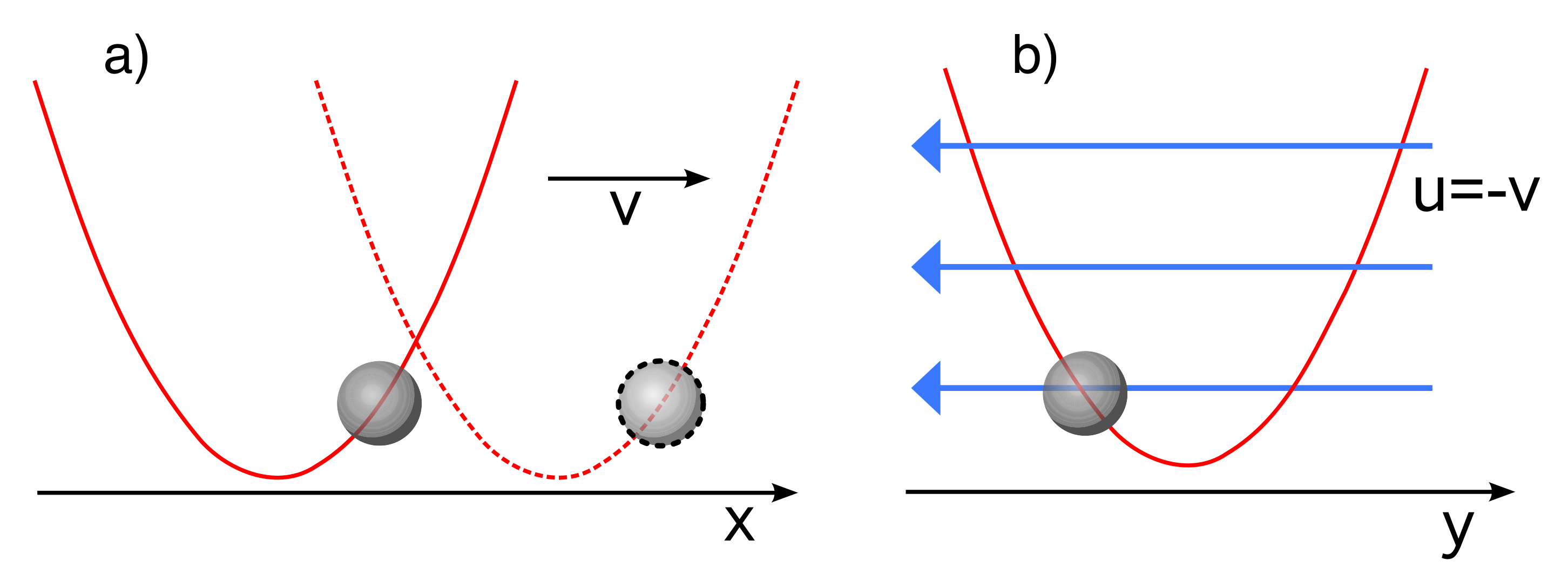
Figure 1: Colloidal particle dragged by optical tweezers through a viscous fluid. a) Laboratory frame of reference. b) Co-moving frame of reference: an observer moving such that the trap appears stationary would see a flow trying to advect the particle. The work is invariant in both scenarios.

To make these ideas transparent and as an example, consider the prototypical colloidal particle dragged by optical tweezers, see Fig. 1. The optical trap is modeled as a harmonic potential with strength $k$ and focus position $\lambda$. This system has been studied comprehensively both theoretically [25, 26] and experimentally [27]. The parameter we control externally is the position of the trap center. Alternatively, one could control the trap strength. The potential energy reads $U(x;\lambda)=(k/2)(x-\lambda)^{2}$ and the work rate following Eq. (5) is $\dot{w}=\dot{\lambda}k(x-\lambda)$, where $x$ is the position of the particle in the laboratory frame. An observer moving with (constant) velocity $v=\dot{\lambda}$ measures the particle position $y=x-vt$. As expected, the expression for the work rate, $\dot{w}=-kyv$, is invariant under such a change of the frame of reference although $\dot{\lambda}=0$ since now the fluid appears to flow with velocity $u=-v$. The corresponding expressions for the heat are $\dot{q}=-k(x-\lambda)\dot{x}=-k(v+\dot{y})$.

The final step is the introduction of a stochastic entropy defined as [10, 13]

$$s(t)\equiv-\ln\psi(x(t),t;\{\lambda_{j}(t)\}).$$ (7)

Averaging this expression leads to the well known Shannon entropy

$$\langle s(t)\rangle=-\int\mathrm{d}x\;\psi(x,t)\ln\psi(x,t).$$ (8)

Taking the time-derivative of Eq. (7), we obtain the balance equation

$$\frac{\mathrm{d}s}{\mathrm{d}t}=-\dot{s}_{\mathrm{med}}+\dot{s}_{\mathrm{tot}},$$ (9)

i.e., the total entropy production rate $\dot{s}_{\mathrm{tot}}$ is the sum of the change of entropy of the system $\mathrm{d}s/\mathrm{d}t$ and the change of medium entropy $\dot{s}_{\mathrm{med}}$. Since we demand the fluid to stay in equilibrium, we can identify the dissipated heat with the change of fluid entropy through the Clausius relation $\dot{s}_{\mathrm{med}}=\dot{q}/T$.

2.3 Discrete state space

Discrete states might be intrinsic but often they arise through some spatial or temporal coarse graining procedure. A biochemically motivated example for the former is the discrete motion of F₁-ATPase [28]. Transitions between states occur with rates $W(x\rightarrow y)$. Analogous to the continuous case discussed in the previous section, the thermodynamic notions of work and heat can be defined consistently [29]. However, stochastic entropy itself might be introduced in a more abstract way regardless of whether the system of interest is coupled to a heat bath [10]. A single stochastic trajectory $x(t)$ of length $t_{\mathrm{obs}}$ consists of $K$ jumps at times $0<t_{\alpha}<t_{\mathrm{obs}}$ from state $x_{\alpha-1}$ to state $x_{\alpha}$ with a given initial state $x_{0}$. The total change of stochastic entropy along this trajectory (in a steady state) can be written

$$\begin{split}\Delta s\equiv s(t_{\mathrm{obs}})-s(0)&=-\sum_{\alpha=1}^{K}\ln\frac{\psi_{0}(x_{\alpha})}{\psi_{0}(x_{\alpha-1})}\\ &=\sum_{\alpha=1}^{K}\ln\frac{W(x_{\alpha}\rightarrow x_{\alpha-1})}{W(x_{\alpha-1}\rightarrow x_{\alpha})}-\sum_{\alpha=1}^{K}\ln\frac{\psi_{0}(x_{\alpha})W(x_{\alpha}\rightarrow x_{\alpha-1})}{\psi_{0}(x_{\alpha-1})W(x_{\alpha-1}\rightarrow x_{\alpha})}\\ &\equiv-s_{\mathrm{med}}[x(t)]+s_{\mathrm{tot}}[x(t)],\end{split}$$ (10)

where in the second line we have expanded the sum by inserting the transition rates. The sums run over all transitions. Following Eq. (9), we interpret the first sum as the change of medium entropy with rate

$$\dot{s}_{\mathrm{med}}(t)=-\sum_{\alpha=1}^{K}\delta(t-t_{\alpha})\ln\frac{W(x_{\alpha}\rightarrow x_{\alpha-1})}{W(x_{\alpha-1}\rightarrow x_{\alpha})}.$$ (11)

The second term in Eq. (10) is the total entropy production. In equilibrium, detailed balance holds with $\psi_{0}(x)W(x\rightarrow y)=\psi_{0}(y)W(y\rightarrow x)$. Hence, in equilibrium the total entropy production becomes identically zero. Moreover, $\langle s_{\mathrm{tot}}\rangle\geqslant 0$, where the equal sign holds in equilibrium. This identification of entropy and the corresponding fluctuation relations for their probability distributions have been illustrated experimentally for a driven single defect in diamond [30, 31].

3 The Fluctuation-Dissipation Theorem

Before discussing the FDT in nonequilibrium, we will briefly introduce an abstract notation particularly apt to treat continuous and discrete state space on equal footing and to see the general structure of the FDT we want to unveil. Using the bra-ket notation, the system is described by the state vector $|\psi(t)\rangle$ from which the probability distribution is read off as $\psi(x,t)=\langle x|\psi(t)\rangle$. We define a reference state $\langle-|$ through $\langle-|\psi(t)\rangle=1$ which expresses the conservation of probability. The time evolution of the state vector is given through

$$\partial_{t}|\psi(t)\rangle=\hat{L}|\psi(t)\rangle$$ (12)

with an operator $\hat{L}$ obeying $\langle-|\hat{L}=0$. The steady state $|\psi_{0}\rangle$ corresponds to the right eigenvector, $\hat{L}|\psi_{0}\rangle=0$, of this time evolution operators with eigenvalue zero. In this picture, the observables correspond to operators with expectation values

$$\langle A(t)\rangle\equiv\langle-|\hat{A}|\psi(t)\rangle.$$ (13)

For diagonal observables, $\langle x|\hat{A}|x^{\prime}\rangle=A(x)\delta(x-x^{\prime})$. This expression reduces to the familiar $\langle A(t)\rangle=\int\mathrm{d}x\;A(x)\psi(x,t)$ upon inserting the identity $\mathbbm{1}=\int\mathrm{d}x\;|x\rangle\langle x|$. Similar expressions where the integration is replaced by a sum are obtained for discrete state spaces. We denote the average value of $A$ in the steady state by $\langle A\rangle_{0}$. Finally, two-point correlations of two observables $A$ and $B$ in the steady state become

$$\langle A(t)B(0)\rangle_{0}\equiv\langle-|\hat{A}e^{t\hat{L}}\hat{B}|\psi_{0}\rangle.$$ (14)

For completeness, we give two explicit expressions for $\hat{L}$. First, the matrix elements of the time-evolution operator for the Smoluchowski equation (2) read

$$\langle x|\hat{L}|x^{\prime}\rangle=-\sum_{k=1}^{N}\nabla_{k}\cdot\left\{\mathbf{u}(\mathbf{r}_{k})+\mu_{0}[-\nabla_{k}U+\mathbf{f}_{k}-T\nabla_{k}]\right\}\delta(x-x^{\prime}).$$ (15)

Second, for a general Markov process on a discrete state space, the time-evolution operator is the usual left stochastic matrix with elements

$$\langle x|\hat{L}|x^{\prime}\rangle=W(x^{\prime}\rightarrow x)-\delta_{xx^{\prime}}\sum_{y\neq x}W(x\rightarrow y).$$ (16)

3.1 Formal derivation

Let $\lambda$ be one control parameter, and without loss of generality let $\lambda=0$ for the steady state. Changing $\lambda$ will perturb the system away from its steady state with the following evolution governed by Eq. (12). For small $\lambda$, the system will response linearly in the sense

$$\langle A(t)\rangle=\langle A\rangle_{0}+\int_{-\infty}^{t}\mathrm{d}t^{\prime}\;R_{A,\lambda}(t-t^{\prime})\lambda(t^{\prime})+\mathcal{O}(\lambda^{2}),$$ (17)

i.e., the mean at later times is a linear functional of the perturbation $\lambda(t)$. The response function $R_{A,\lambda}(t)$ connecting both is formally given through

$$R_{A,\lambda}(t-t^{\prime})\equiv\left.\frac{\delta\langle A(t)\rangle}{\delta\lambda(t^{\prime})}\right|_{\lambda=0}\qquad(t^{\prime}\leqslant t).$$ (18)

Due to causality, the response function vanishes for $t^{\prime}>t$.

The calculation of the response function (18) for general Markovian processes is well known. For completeness and later reference, we repeat the derivation here, following the route of Agarwal [32] and Hänggi and Thomas [33]. The formal solution of Eq. (12) for a, due to the perturbation, time-dependent $\hat{L}(t)$ reads

$$|\psi(t)\rangle=e_{+}^{\int_{-\infty}^{t}\mathrm{d}t^{\prime}\;\hat{L}(t^{\prime})}|\psi_{0}\rangle$$ (19)

given that the system at $t\rightarrow-\infty$ has been prepared in the steady state. The exponential is to be understood in the time-ordered sense. We then split the time evolution operator, $\hat{L}(t)=\hat{L}+\lambda(t)\delta\hat{L}$, and use the expression (13) to obtain

$$R_{A,\lambda}(t-t^{\prime})=\langle-|\hat{A}e^{(t-t^{\prime})\hat{L}}\delta\hat{L}|\psi_{0}\rangle=\langle A(t)B(t^{\prime})\rangle_{0}$$ (20)

after performing the functional derivative with respect to $\lambda(t^{\prime})$. Hence, the response function can be expressed as a correlation function of the observable $A$ with the operator $\delta\hat{L}$. Although formally correct, it is of little practical use as long as we do not find a ’physical’ representation $B$ of this observable in the sense that it can be expressed in terms of, in principle, measurable quantities. For a first representation, we assume the observable $\delta\hat{L}$ to be diagonal, $\delta\hat{L}=\int\mathrm{d}x\;|x\rangle B^{\mathrm{(a)}}(x)\langle x|$, with

$$B^{\mathrm{(a)}}(x)\equiv\frac{\langle x|\delta\hat{L}|\psi_{0}\rangle}{\langle x|\psi_{0}\rangle}.$$ (21)

This result indeed has been known for more than thirty years and we call it the ’Agarwal’ form. However, $B^{\mathrm{(a)}}$ still seems to have no transparent physical meaning. Moreover, for complex systems with a large number of degrees of freedom, the explicit form of the stationary distribution $\psi_{0}(x)$ in general is neither available experimentally nor from numerical simulations.

In the next subsections we will discuss two more representations of $B$ labeled by different superscripts $B^{(i)}$. To this end it is crucial to realize that a whole class of representations for the observable $B$ exist that all lead to the same FDT (20). The formal reason is that we have some freedom in expressing the state $\delta\hat{L}|\psi_{0}\rangle$. Beyond the representations discussed below, there are in principle infinitely many variants of the FDT since with $B^{(1)}\cong B^{(2)}$, where $\cong$ denotes the equivalence of observables, any normalized linear combination

$$\frac{1}{c_{1}+c_{2}}\left[c_{1}B^{(1)}+c_{2}B^{(2)}\right]$$ (22)

with $c_{1,2}$ real will be admissible.

3.2 Role of stochastic entropy

We want to establish the connection between the stochastic entropy (7) and the FDT [21]. We consider two steady states separated by a small $\lambda$ with state vectors $|\psi_{0}\rangle$ and $|\psi_{0}\rangle+\lambda|\delta\psi\rangle$, respectively. Using that these state vectors are the right eigenvectors of the corresponding evolution operators with eigenvalue zero,

$$\hat{L}|\delta\psi\rangle=-\delta\hat{L}|\psi_{0}\rangle$$ (23)

holds to first order in $\lambda$. Inserting this into Eq. (20), we obtain

$$R_{A,\lambda}(t-t^{\prime})=\frac{\partial}{\partial t^{\prime}}\langle-|\hat{A}e^{(t-t^{\prime})\hat{L}}|\delta\psi\rangle=\langle A(t)B^{\mathrm{(e)}}(t^{\prime})\rangle_{0}$$ (24)

which is independent of $\delta\hat{L}$. The physical observable is now given as

$$B^{\mathrm{(e)}}(x,\dot{x})=\frac{\mathrm{d}}{\mathrm{d}t}\frac{\delta\psi(x)}{\psi_{0}(x)}=-\left.\frac{\partial}{\partial\lambda}\frac{\mathrm{d}s}{\mathrm{d}t}\right|_{\lambda=0}.$$ (25)

The total time derivative in the first expression is along a single trajectory starting at $x$. One should keep in mind that this expression is to be averaged over trajectories in the correlation function (27). Expanding Eq. (7) up to first order in $\lambda$ leads to $-\delta\psi(x)/\psi_{0}(x)$ and, finally, we interchange the order of derivations to obtain $B^{\mathrm{(e)}}$. In contrast to Eq. (21), $B^{\mathrm{(e)}}$ in general depends also on $\dot{x}$ and hence is a non-diagonal observable.

The conceptual advantage of Eq. (25) is that it leads to an observable which is conjugate to the perturbation parameter with respect to entropy production, in the same spirit that the observable $B^{\mathrm{(eq)}}$ is conjugate with respect to energy in equilibrium. To recover the equilibrium form (1) of the FDT, we employ the stationary distribution in equilibrium given by the Gibbs-Boltzmann distribution

$$\psi_{0}(x;\lambda)=e^{-[U(x;\lambda)-\mathcal{F}(\lambda)]/T},$$ (26)

where $\mathcal{F}$ is the free energy. The system entropy simply becomes $Ts(t)=U(x(t))-\mathcal{F}$. Eq. (24) then reads

$$TR^{\mathrm{(eq)}}_{A,\lambda}(t-t^{\prime})=\frac{\partial}{\partial t^{\prime}}\langle A(t)[-\partial_{\lambda}U]_{\lambda=0}(t^{\prime})\rangle_{0}+\frac{\partial}{\partial t^{\prime}}\left[\langle A\rangle_{0}\frac{\mathrm{d}\mathcal{F}}{\mathrm{d}\lambda}\right].$$ (27)

The free energy is constant along trajectories. The term in the square brackets is then constant and the second term vanishes. The expression $\partial_{\lambda}s=(1/T)\partial_{\lambda}U$ appears in the FDT, which acquires the well-known form (1). Hence, we can identify $B^{\mathrm{(eq)}}(x)=-\left.\partial_{\lambda}U(x;\lambda)\right|_{\lambda=0}$ as expected.

Considering the general case of a nonequilibrium steady state, the observable (25) can be used to find a link to the equilibrium case (1). Using Eq. (9), we split

$$B^{\mathrm{(e)}}=\partial_{\lambda}\dot{s}_{\mathrm{med}}-\partial_{\lambda}\dot{s}_{\mathrm{tot}}$$ (28)

into two terms. In Ref. [21] it has been shown that the second term vanishes in equilibrium. Hence, in equilibrium the FDT (20) can then also be written in the form

$$R^{\mathrm{(eq)}}_{A,\lambda}(t-t^{\prime})=\langle A(t)[\partial_{\lambda}\dot{s}_{\mathrm{med}}](t^{\prime})\rangle_{0}.$$ (29)

Now consider the same system driven into a nonequilibrium steady state by a driving force corresponding to the parameter $\lambda$. Perturbing the system by a small change of the same driving force will leave $\partial_{\lambda}\dot{s}_{\mathrm{med}}$ unaltered. We can thus keep the correlation function on the right hand side of Eq. (29), now evaluated under nonequilibrium conditions, and subtract the second term in Eq. (28) that involves the observable conjugate to total entropy production to obtain

$$R_{A,\lambda}(t-t^{\prime})=\langle A(t)[\partial_{\lambda}\dot{s}_{\mathrm{med}}](t^{\prime})\rangle_{0}-\langle A(t)[\partial_{\lambda}\dot{s}_{\mathrm{tot}}](t^{\prime})\rangle_{0}.$$ (30)

The second correlation function quantifies the excess compared to equilibrium. Such a splitting has been mentioned before [18, 34] without recognizing the meaning of the excess term as a correlation with the total entropy production. Harada and Sasa have discussed the connection of this excess with energy dissipation [35].

3.3 Path weight approach

An alternative way to write the average (13) is to use the path integral formalism leading to

$$\langle A(t)\rangle=\int\mathrm{d}x\;A(x)\int^{x(t)=x}[\mathrm{d}x(t)]\;P[x(t);\lambda(t)],$$ (31)

where the path integral runs over all trajectories which end in $x$ at time $t$. The weight of a single trajectory is $P[x(t)]=e^{-S[x(t)]}$ with stochastic action $S$. Calculating the response function (18) by taking the functional derivative, we obtain

$$R_{A,\lambda}(t-t^{\prime})=\int\mathrm{d}x\mathrm{d}x^{\prime}\;A(x)\int_{x(t^{\prime})=x^{\prime}}^{x(t)=x}[\mathrm{d}x(t)]\;P_{0}[x(t)]B^{(\mathrm{p})}(x^{\prime},\dot{x}^{\prime})\psi_{0}(x^{\prime}),$$ (32)

where $P_{0}$ is the path weight in the steady state and the path integral now sums over all paths starting in $x^{\prime}$ at earlier time $t^{\prime}$ and ending in $x$ at time $t$. We therefore again find the FDT in the general form (20) but now with the observable representation

$$B^{\mathrm{(p)}}(x,\dot{x})=-\left.\frac{\delta S[x(t);\lambda(t)]}{\delta\lambda(t^{\prime})}\right|_{\lambda=0}=-\partial_{\lambda}\mathcal{L}(x,\dot{x}).$$ (33)

For the last equality, we have used that the action can be written as $S=\int\mathrm{d}t\;\mathcal{L}$. The explicit expressions read

$$\mathcal{L}(t)=\frac{1}{4\mu_{0}T}\sum_{k=1}^{N}[\boldsymbol{\xi}_{k}(t)]^{2}$$ (34)

with $\boldsymbol{\xi}_{k}$ given through the Langevin equation (4) and

$$\mathcal{L}(t)=\sum_{y}W(x(t)\rightarrow y)-\sum_{\alpha=1}^{K}\delta(t-t_{\alpha})\ln W(x_{\alpha-1}\rightarrow x_{\alpha})$$ (35)

for continuous and discrete state space, respectively.

A similar approach has been used by Baiesi et al. to derive yet another form of the FDT by relating the path weight of the perturbed process with the stationary path weight [36]. However, certain forms of this FDT have been know for a long time [37, 19]. For example, realizing that a force perturbation is equivalent to a perturbation of the noise leads immediately to

$$TR_{A,\mathbf{f}_{k}}(t-t^{\prime})=\mu_{0}\left\langle\frac{\delta A(t)}{\delta\boldsymbol{\xi}_{k}(t^{\prime})}\right\rangle=\frac{1}{2}\langle A(t)\boldsymbol{\xi}_{k}(t^{\prime})\rangle.$$ (36)

This has been exploited in Ref. [38].

3.4 Hatano-Sasa relation approach

The term steady state thermodynamics has been coined for a phenomenological theory [39, 40] promoting the splitting of the total dissipated heat into a housekeeping heat $q_{\mathrm{hk}}$ and an excess heat $q_{\mathrm{ex}}$. We introduce a pseudo-potential $\phi(x)$ via the steady state probability

$$\psi_{0}(x)=e^{-\phi(x)},\qquad\phi(x)\neq U(x)/T$$ (37)

in analogy to, but different from, the Gibbs-Boltzmann distribution. The excess heat is $q_{\mathrm{ex}}/T=Y-\Delta\phi$, where $Y$ is the transition functional defined as

$$Y[x(t)]\equiv\int\mathrm{d}t\;\dot{\lambda}_{i}(t)\frac{\partial\phi(x(t);\{\lambda(t)\})}{\partial\lambda_{i}}.$$ (38)

For this transition functional, the fluctuation relation

$$\langle e^{-Y}\rangle=1$$ (39)

holds [41]. For completeness, note that also the housekeeping heat $q_{\mathrm{hk}}\equiv q-q_{\mathrm{ex}}$ fulfills a fluctuation relation [42].

We define the variables

$$X_{j}\equiv-\frac{\partial\phi}{\partial\lambda_{j}}$$ (40)

conjugate to the parameter $\lambda_{j}$ with respect to the pseudo-potential $\phi$. Expanding the Hatano-Sasa relation (39) in powers of the $\lambda$’s, Prost et al. [43] derived the FDT

$$\langle X_{j}\rangle=\int_{-\infty}^{t}\mathrm{d}t^{\prime}\;R_{jk}(t-t^{\prime})\lambda_{k}(t^{\prime}),\qquad R_{jk}(t-t^{\prime})=-\partial_{t}\langle X_{j}(t)X_{k}(t^{\prime})\rangle_{0},$$ (41)

where $\langle X_{j}\rangle_{0}=0$ by construction. Noting that in a steady state the stochastic entropy (7) becomes $s(t)=\phi(x(t))$, we see that this result is equivalent to the FDT (24). However, Eq. (24) seems to be more general since it does not restrict the observable that measures the response.

4 Illustrations

For an illustration, we consider two systems that have been discussed in detail previously [44, 21]: sheared soft matter systems and a single particle moving in a periodic potential.

4.1 Shear driven systems

The system consists of $N$ particles with positions $x\equiv\{\mathbf{r}_{1},\dots,\mathbf{r}_{n}\}$. The FDT in such shear driven suspensions has been addressed numerically [45, 46] and in the framework of mode-coupling theory [14, 47]. Invariant quantities [48] constitute an exact result for systems driven through boundaries with an otherwise unaltered Hamiltonian. In contrast, in this example the system is driven through an imposed flow with profile $\mathbf{u}(\mathbf{r})=(\gamma y,0,0)^{T}$, where $\gamma$ is the strain rate. Shearing the fluid builds up stress with off-diagonal element

$$\sigma_{xy}(x)\equiv\sum_{k=1}^{N}y_{k}\frac{\partial U}{\partial x_{k}},$$ (42)

which will be the crucial quantity in the following.

The time-evolution operator is given by Eq. (15). Perturbing the strain rate $\lambda\mapsto\gamma$, we obtain $\delta L=-\sum_{k=1}^{N}y_{k}\frac{\partial}{\partial x_{k}}$. The first representation of the conjugate observable is the diagonal ’Agarwal’ form (21)

$$TB^{\mathrm{(a)}}(x)=T\frac{\delta L\psi_{0}(x)}{\psi_{0}(x)}=\sigma_{xy}(x)-\bar{\sigma}_{xy}(x).$$ (43)

The second term here is

$$\bar{\sigma}_{xy}(x)\equiv\sum_{k=1}^{N}[U(x)-T\phi(x)]=-\frac{1}{\mu_{0}}\sum_{k=1}^{N}y_{k}(\nu_{k,x}-\gamma y_{k}),$$ (44)

which involves the $x$-component of the local mean velocity (3). The medium entropy production rate following Eq. (6) is

$$T\dot{s}_{\mathrm{med}}=\sum_{k=1}^{N}[\dot{\mathbf{r}}_{k}-\mathbf{u}(\mathbf{r}_{k})]\cdot(\nabla_{k}U)$$ (45)

and therefore $T\partial_{\gamma}\dot{s}_{\mathrm{med}}=\sigma_{xy}$. The representation $B^{\mathrm{(e)}}$ based on the splitting of the entropy production (28) is therefore also diagonal and has to coincide with the first form, $B^{\mathrm{(e)}}=B^{\mathrm{(a)}}$. A different representation is obtained as

$$TB^{\mathrm{(p)}}=\sum_{k}\frac{1}{2\mu_{0}}\left(\dot{x}_{k}+\mu_{0}\frac{\partial U}{\partial x_{k}}-\gamma y_{k}\right)y_{k}=\frac{1}{2}\sigma_{xy}+\frac{1}{2\mu_{0}}\sum_{k}y_{k}(\dot{x}_{k}-\gamma y_{k})$$ (46)

following the path integral approach (33) with Eq. (34). Combining the two different forms, we arrive at

$$T[2B^{\mathrm{(p)}}-B^{\mathrm{(a)}}]=\frac{1}{\mu_{0}}\sum_{k=1}^{N}y_{k}(\dot{x}_{k}-\nu_{k,x}).$$ (47)

This expression also quantifies some kind of stress, where the velocity in $x$-direction is measured with respect to the flow.

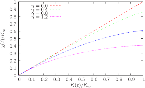
Figure 2: Rouse polymer: The integrated response $\chi(t)$ [Eq. (48)] plotted vs the integrated correlation function $K(t)$ [Eq. (49)] for different strain rates $\gamma$ and normalized by $K_{\infty}\equiv K(t\rightarrow\infty)$. In equilibrium ($\gamma=0$), this plot is a straight line with $T\chi(t)=K(t)$.

Knowing the different representations the FDT can acquire might help to measure, but of course does not specify, the actual functions $R(t)$, $C(t)$, and $I(t)$. Explicit expressions for response and correlation functions have been obtained for the case of a Rouse polymer [49] in Ref. [44]. The potential energy reads $U(x)=(k/2)\sum_{k=1}^{N-1}|\mathbf{r}_{k+1}-\mathbf{r}_{k}|^{2}$. In the limit $N\rightarrow\infty$, the following expressions for integrated response and stress auto correlations have been calculated,

$$\chi(t)\equiv\int_{0}^{\infty}\mathrm{d}t\;R_{\sigma_{xy},\gamma}(t)=T\left[(1-e^{-t})+\sqrt{\pi t}\operatorname{erfc}(\sqrt{t})\right],$$ (48)

$$K(t)\equiv\int_{0}^{\infty}\mathrm{d}t\;\left[\langle\sigma_{xy}(t)\sigma_{xy}(0)\rangle-\langle\sigma_{xy}\rangle^{2}\right]=T^{2}\left[(1+\gamma^{2})(1-e^{-t})+\sqrt{\pi t}\operatorname{erfc}(\sqrt{t})\right].$$ (49)

Here, the time $t$ has been scaled by the fundamental relaxation time $\tau_{1}\equiv(2\mu_{0}k)^{-1}$. In Fig. 2, the integrated response $\chi(K)$ as function of the integrated correlation is plotted for different strain rates $\gamma$. While for $\gamma=0$ we observe a straight line corresponding to $T\chi(t)=K(t)$, the excess and therefore the deviation from the straight line increase with increasing strain rate $\gamma$.

4.2 Single particle in a periodic potential

Another example we have studied previously is that of a driven single colloidal particle moving in one dimension in a periodic potential [38, 21]. The Langevin equation reads

$$\dot{x}=\mu_{0}[-\partial_{x}U(x)+f]+\xi\equiv\mu_{0}F(x)+\xi.$$ (50)

Here we choose $\lambda\mapsto f$, i.e., we perturb the driving force $f$. The perturbation operator $\delta L=-\mu_{0}\partial_{x}$ with Eq. (21) produces the diagonal Agarval form $B^{\mathrm{(a)}}(x)=\nu(x)-\mu_{0}F(x)$. Following the path weight approach leads to $B^{\mathrm{(p)}}(x,\dot{x})=(1/2)[\dot{x}-\mu_{0}F(x)]$. A straightforward combination of both results amounts to

$$B^{\mathrm{(e)}}=2B^{\mathrm{(p)}}-B^{\mathrm{(a)}}=\dot{x}-\nu.$$ (51)

Since form Eq. (6) $T\partial_{f}\dot{s}_{\mathrm{med}}=\dot{x}$ follows we can identify $T\partial_{f}\dot{s}_{\mathrm{tot}}\cong\nu$, i.e., the excess involves as observable the local mean velocity (3). The idea of identifying the excess with the local mean velocity has lead to a formulation where the FDT acquires its equilibrium form through a transformation into the Lagrangian reference frame moving with the local mean velocity [50, 51, 52]. Fluctuations in this co-moving frame are essentially equilibrium fluctuations and the driving manifests itself in the mean values of observables. Of course, this result also crucially depends on fixing the bath fluctuations to be equilibrium fluctuations.

5 Summary

In summary, the general FDT for Markovian dynamics is considered. Following Ref. [21], a generalized FDT is derived where the conjugate observable is determined with respect to entropy production of the system in contrast to equilibrium where the conjugate observable is determined with respect to energy. Alternative ways to derive generalized FDTs for driven systems are sketched based on the path-integral and on the Hatano-Sasa relation (39). It is shown how the results of different approaches can be combined to produce new conjugate observables through linear combination. The general theory is illustrated for shear driven systems where the strain rate is the perturbation parameter and a driven single colloidal particle with the driving force taking the role as the perturbation parameter.

References

- [1] R. Kubo, M. Toda, and N. Hashitsume, Statistical Physics II, 2nd ed. (Springer-Verlag, Berlin, 1991).
- [2] S. R. de Groot and P. Mazur, Non-equilibrium thermodynamics (North-Holland, Amsterdam, 1962).
- [3] C. Jarzynski, Phys. Rev. Lett. 78, 2690 (1997).
- [4] C. Jarzynski, Phys. Rev. E 56, 5018 (1997).
- [5] G. E. Crooks, Phys. Rev. E 60, 2721 (1999).
- [6] G. E. Crooks, Phys. Rev. E 61, 2361 (2000).
- [7] D. J. Evans, E. G. D. Cohen, and G. P. Morriss, Phys. Rev. Lett. 71, 2401 (1993).
- [8] G. Gallavotti and E. G. D. Cohen, Phys. Rev. Lett. 74, 2694 (1995).
- [9] D. J. Evans and D. J. Searles, Adv. Phys. 51, 1529 (2002).
- [10] U. Seifert, Phys. Rev. Lett. 95, 040602 (2005).
- [11] C. Bustamante, J. Liphardt, and F. Ritort, Physics Today 58(7), 43 (2005).
- [12] F. Ritort, Adv. Chem. Phys. 137, 31 (2007).
- [13] U. Seifert, Eur. Phys. J. B 64, 423 (2008).
- [14] G. Szamel, Phys. Rev. Lett. 93, 178301 (2004).
- [15] V. Blickle, T. Speck, L. Helden, U. Seifert, and C. Bechinger, Phys. Rev. Lett. 96, 070603 (2006).
- [16] T. Speck, V. Blickle, C. Bechinger, and U. Seifert, EPL 79, 30002 (2007).
- [17] V. Blickle, T. Speck, C. Lutz, U. Seifert, and C. Bechinger, Phys. Rev. Lett. 98, 210601 (2007).
- [18] A. Crisanti and F. Ritort, J. Phys. A: Math. Gen. 36, R181 (2003).
- [19] P. Calabrese and A. Gambassi, J. Phys. A: Math. Gen. 38, R133 (2005).
- [20] U. M. B. Marconi, A. Puglisi, L. Rondoni, and A. Vulpiani, Phys. Rep. 461, 111 (2008).
- [21] U. Seifert and T. Speck, arXiv:0907.5478 (2009).
- [22] K. Sekimoto, J. Phys. Soc. Jpn. 66, 1234 (1997).
- [23] K. Sekimoto, Prog. Theor. Phys. Supp. 130, 17 (1998).
- [24] T. Speck, J. Mehl, and U. Seifert, Phys. Rev. Lett. 100, 178302 (2008).
- [25] R. van Zon and E. G. D. Cohen, Phys. Rev. E 67, 046102 (2003).
- [26] T. Speck and U. Seifert, Eur. Phys. J. B 43, 521 (2005).
- [27] E. H. Trepagnier, C. Jarzynski, F. Ritort, G. E. Crooks, C. J. Bustamante, and J. Liphardt, Proc. Natl. Acad. Sci. U.S.A. 101, 15038 (2004).
- [28] R. Yasuda, H. Noji, K. Kinosita, and M. Yoshida, Cell 93, 1117 (1998).
- [29] T. Schmiedl and U. Seifert, J. Chem. Phys. 126, 044101 (2007).
- [30] S. Schuler, T. Speck, C. Tietz, J. Wrachtrup, and U. Seifert, Phys. Rev. Lett. 94, 180602 (2005).
- [31] C. Tietz, S. Schuler, T. Speck, U. Seifert, and J. Wrachtrup, Phys. Rev. Lett. 97, 050602 (2006).
- [32] G. S. Agarwal, Z. Physik 252, 25 (1972).
- [33] P. Hänggi and H. Thomas, Phys. Rep. 88, 207 (1982).
- [34] G. Diezemann, Phys. Rev. E 72, 011104 (2005).
- [35] T. Harada and S. Sasa, Phys. Rev. Lett. 95, 130602 (2005).
- [36] M. Baiesi, C. Maes, and B. Wynants, Phys. Rev. Lett. 103, 010602 (2009).
- [37] L. F. Cugliandolo, J. Kurchan, and G. Parisi, J. Phys. I 4, 1641 (1994).
- [38] T. Speck and U. Seifert, Europhys. Lett. 74, 391 (2006).
- [39] Y. Oono and M. Paniconi, Prog. Theor. Phys. Suppl. 130, 29 (1998).
- [40] S. ichi Sasa and H. Tasaki, J. Stat. Phys. 125, 125 (2006).
- [41] T. Hatano and S. Sasa, Phys. Rev. Lett. 86, 3463 (2001).
- [42] T. Speck and U. Seifert, J. Phys. A: Math. Gen. 38, L581 (2005).
- [43] J. Prost, J.-F. Joanny, and J. M. R. Parrondo, Phys. Rev. Lett. 103, 090601 (2009).
- [44] T. Speck and U. Seifert, Phys. Rev. E 79, 040102 (2009).
- [45] J. L. Barrat and L. Berthier, Phys. Rev. E 63, 012503 (2000).
- [46] L. Berthier and J.-L. Barrat, J. Chem. Phys. 116, 6228 (2002).
- [47] M. Krüger and M. Fuchs, Phys. Rev. Lett. 102, 135701 (2009).
- [48] A. Baule and R. M. L. Evans, Phys. Rev. Lett. 101, 240601 (2008).
- [49] M. Doi, Introduction to Polymer Physics (Clarendon Press, Oxford, 1996).
- [50] R. Chetrite, G. Falkovich, and K. Gawedzki, J. Stat. Mech.: Theor. Exp. P08005 (2008).
- [51] R. Chetrite and K. Gawedzki, cond-mat 0905.4667 (2009).
- [52] J. R. Gomez-Solano, A. Petrosyan, S. Ciliberto, R. Chetrite, and K. Gawedzki, Phys. Rev. Lett. 103, 040601 (2009).
- [53] T. Speck, Ph.D. thesis, Universität Stuttgart, 2007.