A class of linear solvers built on the Biconjugate $A$-Orthonormalization Procedure for solving unsymmetric linear systems

Abstract

We present economical iterative algorithms built on the Biconjugate $A$-Orthonormalization Procedure for real unsymmetric and complex non-Hermitian systems. The principal characteristics of the developed solvers is that they are fast convergent and cheap in memory. We report on a large combination of numerical experiments to demonstrate that the proposed family of methods is highly competitive and often superior to other popular algorithms built upon the Arnoldi method and the biconjugate Lanczos procedures for unsymmetric linear sytems.

Key words: Biconjugate $A$-Orthonormalization Procedure; Krylov subspace methods; Linear systems; Sparse and Dense Matrix Computation.

AMSC: 65F10

1 Introduction

In this study we investigate variants of the Lanczos method for the iterative solution of real unsymmetric and/or complex non-Hermitian linear systems

$$Ax=b,$$ (1)

with the motivation of obtaining smoother and, hopefully, faster convergence behavior in comparison with the BiCG method as well as its two evolving variants - the CGS method and one of the most popular methods in use today - the Biconjugate Gradient Stabilized (BiCGSTAB) method.

Iterative methods for solving unsymmetric systems are commonly developed upon the Arnoldi or the Lanczos biconjugate algorithms. These procedures generate an orthonormal basis for the Krylov subspaces associated with $A$ and an initial vector $v$, and require only matrix-vector products by $A$. The generation of the vector recurrence by Arnoldi produces Hessenberg matrices, while the unsymmetric Lanczos biconjugation produces tridiagonal matrices. The price to pay due long recurrences in Arnoldi is the increasing orthogonalization cost along the iterations. In this paper we develop economical iterative algorithms built on the Biconjugate $A$-Orthonormalization Procedure presented in Section 2. The method ideally builds up a pair of Biconjugate $A$-Orthonormal (or, briefly, $A$-biorthonormal) basis for the dual Krylov subspaces $K_{m}(A;v_{1})$ and $A^{T}K_{m}(A^{T};w_{1})$ in the real case (which is $A^{H}K_{m}(A^{H};w_{1})$ in the complex case). The projection matrix onto the corresponding Krylov subspace is tridiagonal, so that the generation of the vector recurrences is extremely cheap in memory. We provide the theoretical background for the developed algorithms and we discuss computational aspects. We show by numerical experiments that the Biconjugate $A$-Orthonormalization Procedure may lead to highly competitive solvers that are often superior to other popular methods, e.g. CGS, BiCGSTAB, IDR($s$). We apply these techniques to sparse and dense matrix problems, both in real and complex arithmetic, arising from realistic applications in different areas. This study integrates and extends the preliminary investigations reported in [12], limited to the case of complex non-Hermitian systems. In this paper we consider a much larger combination of experiments with both real and complex matrices having size order twice as large. Finally, we complete our work with a case study with dense linear systems in electromagnetic scattering from large structures.

The paper is structured as follows: in Section 2 we present the Biconjugate $A$-Orthonormalization Procedure and its properties; in Section 3 we describe a general framework to derive linear solver from the proposed procedure, and we present the algorithmic development of two Krylov projection algorithms. Finally, in Section 6 we report on extensive numerical experiments for solving large sparse and/or dense linear systems, both real and complex.

2 A general two-sided unsymmetric Lanczos biconjugate A-orthonormalization procedure

Throughout this paper we denote the standard inner product of two real vectors $u,v\in\mathbb{R}^{n}$ as

$$\left\langle{u,v}\right\rangle=u^{T}v=\sum\limits_{i=1}^{n}{u_{i}v_{i}}.$$

Given two vectors $v_{1}$ and $w_{1}$ with euclidean inner product $\left\langle{\omega_{1},Av_{1}}\right\rangle=1$, we define Lanczos-type vectors $v_{j}$, $w_{j}$ and scalars $\delta_{j}$, $\beta_{j}$, $j=1,2,\ldots,m$ by the following recursions

$$\delta_{j+1}v_{j+1}=Av_{j}-\beta_{j}v_{j-1}-\alpha_{j}v_{j}=s_{j+1},$$ (2)

$$\beta_{j+1}w_{j+1}=A^{T}w_{j}-\delta_{j}w_{j-1}-\alpha_{j}w_{j}=t_{j+1}.$$ (3)

where the scalars are chosen as

$$\alpha_{j}=\left\langle{\omega_{j},A\left({Av_{j}}\right)}\right\rangle,~{}\displaystyle\delta_{j+1}=\left|{\left\langle{\hat{\omega}_{j+1},A\hat{v}_{j+1}}\right\rangle}\right|^{\frac{1}{2}},~{}\displaystyle\beta_{j+1}=\frac{\left\langle{\hat{\omega}_{j+1},A\hat{v}_{j+1}}\right\rangle}{\delta_{j+1}}.$$

This choice of the scalars guarantees that the recursions generate sequences of biconjugate $A$-orthonormal vector (or briefly, $A$-biorthonormal vectors) $v_{i}$ and $w_{i}$, according to the following definition

Definition 1

Right and left Lanczos-type vectors $v_{j},~{}j=1,2,\ldots,m$ and $w_{i},~{}i=1,2,\ldots,m$ form a biconjugate A-orthonormal system in exact arithmetic, if and only if

$$\left\langle{\omega_{i},Av_{j}}\right\rangle=\delta_{i,j},~{}1\leq i,j\leq m.$$

$\blacksquare$

Eqns. (2-3) can be interpreted as a two-side Gram-Schmidt orthonormalization procedure where at step $i$ we multiply vectors $v_{i}$ and $w_{i}$ by $A$ and $A^{T}$, respectively, and we orthonormalize them against the most recently generated Lanczos-type pairs $(v_{i},w_{i})$ and $(v_{i-1},w_{i-1})$. The vectors $\alpha_{i}v_{i}$, $\alpha_{i}w_{i}$ are the complex biconjugate $A$-orthonormal projections of $Av_{i}$ and $A^{T}w_{i}$ onto the most recently computed vectors $v_{i}$ and $w_{i}$; analogously, the vectors $\beta_{i}v_{i-1}$, $\delta_{i}w_{i-1}$ are the complex biconjugate $A$-orthonormalization projections of $Av_{i}$ and $A^{T}w_{i}$ onto the next computed vectors $v_{i-1}$ and $w_{i-1}$. The two sets of scalars satisfy the following relation

$$\beta_{i+1}\delta_{i+1}=s_{i+1}^{T}At_{i+1}=\left\langle{s_{i+1},At_{i+1}}\right\rangle.$$

The scalars $\beta_{i}$ and $\delta_{i}$ can be chosen with some freedom, provided the biconjugate $A$-orthonormalization property holds. We sketch the complete procedure in Algorithm 1

Algorithm 1 The Lanczos A-biorthonormalization procedure

1:  Choose $v_{1},\omega_{1}$, such that $\left\langle{\omega_{1},Av_{1}}\right\rangle=1$

2:  Set $\beta_{1}=\delta_{1}\equiv 0,\omega_{0}=v_{0}={\bf 0}\in\mathbb{R}^{n}$

3:  for $j=1,2,\ldots$ do

4:     $\alpha_{j}=\left\langle{\omega_{j},A\left({Av_{j}}\right)}\right\rangle$

5:     $\hat{v}_{j+1}=Av_{j}-\alpha_{j}v_{j}-\beta_{j}v_{j-1}$

6:     $\hat{\omega}_{j+1}=A^{T}\omega_{j}-\alpha_{j}\omega_{j}-\delta_{j}\omega_{j-1}$

7:     $\displaystyle\delta_{j+1}=\left|{\left\langle{\hat{\omega}_{j+1},A\hat{v}_{j+1}}\right\rangle}\right|^{\frac{1}{2}}$

8:     $\displaystyle\beta_{j+1}=\frac{\left\langle{\hat{\omega}_{j+1},A\hat{v}_{j+1}}\right\rangle}{\delta_{j+1}}$

9:     $\displaystyle v_{j+1}=\frac{{\hat{v}_{j+1}}}{{\delta_{j+1}}}$

10:     $\displaystyle\omega_{j+1}=\frac{{\hat{\omega}_{j+1}}}{{\beta_{j+1}}}$

11:  end for

Notice that there is a clear analogy with the standard unsymmetric biconjugate Lanczos recursions. The matrix $A$ is not modified and is accessed only via matrix-vector products by $A$ and $A^{T}$. Similarly to the standard Lanczos procedure, the two most recently computed pairs of Lanczos-type vectors $v_{k}$ and $w_{k}$ for $k=i,i-1$ are needed at each step. These two vectors may be overwritten with the most recent updates. Therefore the memory storage is very limited compared to the Arnoldi method. The price to pay is some lack of robustness due to possible vanishing of the inner products. Observe that the above algorithm is possible to breakdown whenever $\delta_{j+1}$ vanishes while $\hat{w}_{j+1}$ and $A\hat{v}_{j+1}$ are not equal to $0\in\mathbb{R}^{n}$ appearing in line 7. In the interest of counteractions against such breakdowns, refer oneself to remedies such as so-called look-ahead strategies [16, 15, 9, 11] which can enhance stability while increasing cost modestly, or others for example [3]. But that is outside the scope of this paper and we shall not pursue that here; for more details, please refer to [18] and the references therein. In our experiments we never observed a breakdown of the algorithm, as we will see in Section 6. However, it is fair to mention that this problem may occurr. The following proposition states some useful properties of Algorithm 1.

Proposition 1

If Algorithm 1 proceeds $m$ steps, then the right and left Lanczos-type vectors $v_{j},j=1,2,\ldots,m$ and $w_{i},i=1,2,\ldots,m$ form a biconjugate A-orthonormal system in exact arithmetic, i.e.,

$$\left\langle{\omega_{i},Av_{j}}\right\rangle=\delta_{i,j},1\leq i,j\leq m.$$

Furthermore, denote by $V_{m}=\left[{v_{1},v_{2},\ldots,v_{m}}\right]$ and $W_{m}=\left[{w_{1},w_{2},\ldots,w_{m}}\right]$ the $n\times m$ matrices and by $\underline{T_{m}}$ the extended tridiagonal matrix of the form

$$\underline{T_{m}}=\left[\begin{array}[]{l}T_{m}\\ \delta_{m+1}e_{m}^{T}\\ \end{array}\right],$$ (4)

where

$$T_{m}=\left[{\begin{array}[]{*{20}c}{\alpha_{1}}&{\beta_{2}}&{}\hfil&{}\hfil&{}\hfil\\ {\delta_{2}}&{\alpha_{2}}&{\beta_{3}}&{}\hfil&{}\hfil\\ {}\hfil&\ddots&\ddots&\ddots&{}\hfil\\ {}\hfil&{}\hfil&{\delta_{m-1}}&{\alpha_{m-1}}&{\beta_{m}}\\ {}\hfil&{}\hfil&{}\hfil&{\delta_{m}}&{\alpha_{m}}\\ \end{array}}\right],$$

whose entries are the coefficients generated during the algorithm implementation, and in which $\alpha_{1},\ldots,\alpha_{m},\beta_{2},\ldots,\beta_{m}$ are complex while $\delta_{2},\ldots,\delta_{m}$ positive. Then with the Biconjugate A-Orthonormalization Procedure, the following four relations hold

$$AV_{m}=V_{m}T_{m}+\delta_{m+1}v_{m+1}e_{m}^{T}$$ (5)

$$A^{T}W_{m}=W_{m}T_{m}^{T}+\beta_{m+1}\omega_{m+1}e_{m}^{T}$$ (6)

$$W_{m}^{T}AV_{m}=I_{m}$$ (7)

$$W_{m}^{T}A^{2}V_{m}=T_{m}$$ (8)

Proof. See [12].

$\blacksquare$

A characterization of Algorithm 1 in terms of projections into relevant Krylov subspaces is derived in the following

Corollary 1

The biconjugate Lanczos $A$-orthonormalization method ideally builds up a pair of biconjugate A-orthonormal bases for the dual Krylov subspaces $K_{m}(A;v_{1})$ and $A^{T}K_{m}(A^{T};w_{1})$. The matrix $T_{m}$ is the projection of the matrix $A$ onto the corresponding Krylov subspaces.

$\blacksquare$

3 The Lanczos $A$-biorthonormalization method for general linear systems

From the recursions defined in Eqns (2)-(3) and the characterization given by Corollary (1), we derive a Lanczos $A$-biorthonormalization method for general linear systems along the following lines.

STEP 1

Run Algorithm 1 $m$ steps for some user specified $m\ll n$ and generate Lanczos-type matrices $V_{m}=[v_{1},v_{2},\ldots,v_{m}]$, $W_{m}=[w_{1},w_{2},\ldots,w_{m}]$ and the tridiagonal projection matrix $T_{m}$ defined in Proposition 1.

STEP 2

Compute the approximate solution $x_{m}$ that belongs to the Krylov subspace $x_{0}+K_{m}(A;v_{1})$ by imposing the residual be orthogonal to the constraint subspace $L_{m}\equiv A^{T}K_{m}(A^{T};w_{1})$

$$r_{m}=b-Ax_{m}~{}\bot~{}L_{m},$$

or equivalently in matrix formulation

$$\left({A^{T}W_{m}}\right)^{T}\left({b-Ax_{m}}\right)=0.$$ (9)

Recall that the approximate solution has form

$$x_{m}=x_{0}+V_{m}y_{m},$$ (10)

so that by simple substitution and computation with Eqns (8-10) we obtain a tridiagonal system to solve for $y_{m}$,

$$T_{m}y_{m}=\beta e_{1},~{}~{}\beta=\left\|{r_{0}}\right\|_{2}.$$ (11)

STEP 3

Compute the new residual and if convergence is observed, terminate the computation. Otherwise, enlarge the Krylov subspace and repeat the process again.

The whole iterative scheme is sketched in Algorithm 2. It solves not only the original linear system $Ax=b$ but, implicitly, also a dual linear system $A^{T}x^{*}=b^{*}$ with $A^{T}$. Analogously, we can derive the counterpart of Algorithm 2 for the solution of the corresponding dual system $A^{T}x^{*}=b^{*}$, where the dual approximation $x_{m}^{*}$ is sought from the affine subspace $x_{0}^{*}+K_{m}\left({A^{T},w_{1}}\right)$ of dimension $m$ satisfying

$$b^{*}-A^{T}x_{m}^{*}~{}~{}\bot~{}~{}AK_{m}\left({A,v_{1}}\right).$$

Denote $r_{0}^{*}=b^{*}-A^{T}x_{0}^{*}$ and $\beta^{*}=\left\|{r_{0}^{*}}\right\|_{2}$. If $w_{1}=\frac{{r_{0}^{*}}}{{\beta^{*}}}$ and $v_{1}$ is chosen properly such that $\left\langle{v_{1},Aw_{1}}\right\rangle=1$, then the counterparts of (9-11) are the following

$$\left({AV_{m}}\right)^{T}\left({b^{*}-A^{T}x_{m}^{*}}\right)=0$$ (12)

$$x_{m}^{*}=x_{0}^{*}+W_{m}y_{m}^{*},$$ (13)

$$T_{m}^{T}y_{m}^{*}=\beta^{*}e_{1}$$ (14)

where $V_{m},W_{m}$ and $T_{m}$ are defined in Proposition 1 and $y_{m}^{*}\in\mathbb{R}^{n}$ is the coefficient vector of the dual linear combination. In Section 6 we will derive a formulation that does not require multiplications by $A^{T}$.

Algorithm 2 Two-sided Biconjugate A-Orthonormalization method.

1:  Compute $r_{0}=b-Ax_{0}$ for some initial guess $x_{0}$ and set $\beta=\left\|{r_{0}}\right\|_{2}$.

2:  Start with $v_{1}=\frac{{r_{0}}}{\beta}$ and choose $\omega_{1}$ such that $\left\langle{\omega_{1},Av_{1}}\right\rangle=1$, (for example, $\omega_{1}=\frac{{Av_{1}}}{{\left\|{Av_{1}}\right\|_{2}^{2}}}$).

3:  Generate the Lanczos-type vectors $V_{m}=\left[{v_{1},v_{2},\ldots,v_{m}}\right]$ and $W_{m}=\left[{w_{1},w_{2},\ldots,w_{m}}\right]$ as well as the tridiagonal matrix $T_{m}$ defined in Proposition 1 by running Algorithm 1 $m$ steps.

4:  Compute $y_{m}=T_{m}^{-1}\left({\beta e_{1}}\right)$ and $x_{m}=x_{0}+V_{m}y_{m}$.

The approximation $x_{m}$ and the dual approximation $x_{m}^{*}$ can be updated respectively from $x_{m-1}$ and $x_{m-1}^{*}$ at each step. Assume the $LU$ decomposition of the tridiagonal matrix $T_{m}$ is

$$T_{m}=L_{m}U_{m},$$

substituting which into (10-11) and (13-14) gives respectively

$$x_{m} =x_{0}+V_{m}\left({L_{m}U_{m}}\right)^{-1}\left({\beta e_{1}}\right)$$

$$=x_{0}+V_{m}U_{m}^{-1}L_{m}^{-1}\left({\beta e_{1}}\right)$$

$$=x_{0}+P_{m}z_{m},$$

$$x_{m}^{*} =x_{0}^{*}+W_{m}\left({U_{m}^{T}L_{m}^{T}}\right)^{-1}\left({\beta^{*}e_{1}}\right)$$

$$=x_{0}^{*}+W_{m}\left({L_{m}^{T}}\right)^{-1}\left({U_{m}^{T}}\right)^{-1}\left({\beta^{*}e_{1}}\right)$$

$$=x_{0}^{*}+P_{m}^{*}z_{m}^{*},$$

where $P_{m}=V_{m}U_{m}^{-1},z_{m}=L_{m}^{-1}\left({\beta e_{1}}\right)$, and $P_{m}^{*}=W_{m}\left({L_{m}^{T}}\right)^{-1},z_{m}^{*}=\left({U_{m}^{T}}\right)^{-1}\left({\beta^{*}e_{1}}\right)$. Using the same argument as in the derivation of DIOM from IOM Algorithm in [18]-Chapter 6, we easily derive the relations

$$x_{m}=x_{m-1}+\zeta_{m}p_{m},$$

$$x_{m}^{*}=x_{m-1}^{*}+\zeta_{m}^{*}p_{m}^{*},$$

where $\xi_{m}$ and $\xi_{m}^{*}$ are coefficients, $p_{m}$ and $p_{m}^{*}$ are the corresponding $m$th column vectors in $P_{m}$ and $P_{m}^{*}$ defined above, termed as the $m$th primary and dual direction vectors, respectively.

Observe that the pairs of the primary and dual direction vectors form a biconjugate $A^{2}$-orthonormal set, i.e., $\left\langle{p_{i}^{*},A^{2}p_{j}}\right\rangle=\delta_{i,j}\left({1\leq i,j\leq m}\right)$, which follows clearly from

$$\left({P_{m}^{*}}\right)^{T}A^{2}P_{m} =\left({W_{m}\left({L_{m}^{T}}\right)^{-1}}\right)^{T}A^{2}V_{m}U_{m}^{-1}$$

$$=L_{m}^{-1}W_{m}^{T}A^{2}V_{m}U_{m}^{-1}$$

$$=L_{m}^{-1}T_{m}U_{m}^{-1}$$

$$=L_{m}^{-1}L_{m}U_{m}U_{m}^{-1}$$

$$=I_{m}$$

with (8). In addition, the $m$th primary residual vector $r_{m}=b-Ax_{m}$ and the $m$th dual residual vector $r_{m}^{*}=b^{*}-Ax_{m}^{*}$ can be expressed as

$$r_{m}=-\delta_{m+1}e_{m}^{T}y_{m}v_{m+1},$$ (15)

$$r_{m}^{*}=-\beta_{m+1}e_{m}^{T}y_{m}^{*}w_{m+1},$$ (16)

by simple computation with (5-6,10-11,13-14). Eqns (15) and (16) together with (7) reveal that the primary and dual residual vectors satisfy the biconjugate $A$-orthogonal conditions, i.e. $\left\langle{r_{i}^{*},Ar_{j}}\right\rangle=0$ for $i\neq j$.

It is known that the constraint subspace in an oblique projection method is different from the search subspace and may be totally unrelated to it. The distinction is rather important and gives rise to different types of algorithms [18]. The biconjugate $A$-orthogonality between the primary and dual residual vectors and the biconjugate $A^{2}$-orthonormality between the primary and dual direction vectors reveal and suggest alternative choices for the constraint subspace. This idea helps to devise the BiCOR method described in the coming section.

4 The BiCOR method

Proceeding in a similar way like the Conjugate Gradient and its variants CG, CR, COCG, BiCGCR, COCR and BiCR, given an initial guess $x_{0}$ to the considered linear system $Ax=b$, we derive algorithms governed by the following coupled two-term recurrences

$$r_{0}=b-Ax_{0},~{}p_{0}=r_{0},$$ (17)

$$x_{j+1}=x_{j}+\alpha_{j}p_{j},$$ (18)

$$r_{j+1}=r_{j}-\alpha_{j}Ap_{j},$$ (19)

$$p_{j+1}=r_{j+1}+\beta_{j}p_{j},~{}\textrm{for}~{}j=0,1,\ldots$$ (20)

where $r_{j}=b-Ax_{j}$ is the $j$th residual vector and $p_{j}$ is the $j$th search direction vector. Denoting $L_{m}$ the underlying constraints subspace, the parameters $\alpha_{i}$, $\beta_{i}$ can be determined by imposing the following orthogonality conditions:

$$r_{j+1}~{}\bot~{}L_{m}\textrm{~{}and~{}}Ap_{j+1}~{}\bot~{}L_{m}.$$ (21)

For concerned real unsymmetric linear systems

$$Ax=b,$$ (22)

an expanded choice for the constraint subspace is $L_{m}=A^{T}K_{m}(A^{T},r_{0}^{*})$, where $r_{0}^{*}$ is chosen to be equal to $P(A)r_{0}$, with $P(t)$ an arbitrary polynomial of certain degree with respect to the variable $t$ and $p_{0}^{*}=r_{0}^{*}$. It should be noted that the optimal choice for the involved polynomial is in general not easily obtainable and requires some expertise and artifice. This aspect needs further research. When there is no ambiguity or other clarification, a specific default choice for $L_{m}$ with $r_{0}^{*}=Ar_{0}$ is adopted in the numerical experiments against the other popular choice for $L_{m}$ with $r_{0}^{*}=r_{0}$, see e.g. [23, 22]. It is important to note that the scalars  $\alpha_{j},\beta_{j}(j=0,1,\ldots)$ in the recurrences (18-20) are different from those produced by Algorithm 1. The search direction vectors $p_{j}^{\prime}s$ here are multiples of the primary direction vectors $p_{j}^{\prime}s$ defined in Section 3. The coupled two-term recurrences for the $(j+1)$th shadow residual vector $r_{j+1}^{*}$ and the associated $(j+1)$th shadow search direction $p_{j+1}^{*}$ can be augmented by similar relations to (19-20) as follows:

$$r_{j+1}^{*}=r_{j}^{*}-\alpha_{j}A^{T}p_{j}^{*},$$ (23)

$$p_{j+1}^{*}=r_{j+1}^{*}+\beta_{j}p_{j}^{*},\textrm{~{}for~{}}j=0,1,\ldots$$ (24)

where $\alpha_{j}$ and $\beta_{j}$ are the conjugate complex of $\alpha_{j}$ and $\beta_{j}$ in (19-20), correspondingly. Then with a certain polynomial $P(t)$ with respect to $t$, (21) explicitly reads

$$r_{j+1}~{}\bot~{}A^{T}K_{m}\left({A^{T},r_{0}^{*}}\right)\textrm{~{}and~{}}Ap_{j+1}~{}\bot~{}A^{T}K_{m}\left({A^{T},r_{0}^{*}}\right)\textrm{~{}with~{}}r_{0}^{*}=P(A)r_{0}$$ (25)

which can be reinterpreted from a practical point of view as

• the residual vectors $r_{i}$’s and the shadow residual vectors $r_{j}^{*}$’s are biconjugate $A$-orthogonal to each other, i.e., $\left\langle{r_{j}^{*},Ar_{i}}\right\rangle=\left\langle{A^{T}r_{j}^{*},r_{i}}\right\rangle=0,$ for $i\neq j$;

• the search direction vectors $p_{i}^{\prime}s$ and the shadow search direction vectors $p_{j}^{*}$’s form an $A^{2}$-biconjugate set, i.e., $\left\langle{p_{j}^{*},A^{2}p_{i}}\right\rangle=\left\langle{A^{T}p_{j}^{*},Ap_{i}}\right\rangle=\left\langle{\left({A^{T}}\right)^{2}p_{j}^{*},p_{i}}\right\rangle=0,$ for $i\neq j$.

These facts are already stated in the latter part of Section 3. Therefore, we possess the conditions to determine the scalars $\alpha_{j}$ and $\beta_{j}$ by imposing the corresponding biorthogonality and biconjugacy conditions (25) into (19-20,23-24). We use extensively the algorithmic schemes introduced in [8] for descriptions of the present algorithms.

Making the inner product of $A^{T}r_{j}^{*}$ and $r_{j+1}$ as defined by (19) yields

$$\left\langle{A^{T}r_{j}^{*},r_{j+1}}\right\rangle=\left\langle{A^{T}r_{j}^{*},r_{j}-\alpha_{j}Ap_{j}}\right\rangle=0,$$

with the biconjugate $A$-orthogonality between $r_{j+1}$ and $r_{J}^{*}$, further resulting in

$$\alpha_{j}=\frac{{\left\langle{A^{T}r_{j}^{*},r_{j}}\right\rangle}}{{\left\langle{A^{T}r_{j}^{*},Ap_{j}}\right\rangle}},$$

where the denominator of the above right-hand side can be further modified as

$$\left\langle{A^{T}r_{j}^{*},Ap_{j}}\right\rangle=\left\langle{A^{T}p_{j}^{*}-\beta_{j-1}A^{T}p_{j-1}^{*},Ap_{j}}\right\rangle=\left\langle{A^{T}p_{j}^{*},Ap_{j}}\right\rangle,$$

because $p_{j-1}^{*}$ and $p_{j}$ are $A^{2}$-biconjugate. Then

$$\alpha_{j}=\frac{{\left\langle{A^{T}r_{j}^{*},r_{j}}\right\rangle}}{{\left\langle{A^{T}p_{j}^{*},Ap_{j}}\right\rangle}}=\frac{{\left\langle{r_{j}^{*},Ar_{j}}\right\rangle}}{{\left\langle{A^{T}p_{j}^{*},Ap_{j}}\right\rangle}}$$ (26)

Similarly, writing that $p_{j+1}$ as defined by (20) is $A^{2}$-biconjugate to $p_{j}^{*}$ yields

$$\left\langle{p_{j}^{*},A^{2}p_{j+1}}\right\rangle=\left\langle{A^{T}p_{j}^{*},Ap_{j+1}}\right\rangle=\left\langle{A^{T}p_{j}^{*},Ar_{j+1}+\beta_{j}Ap_{j}}\right\rangle=0,$$

giving

$$\beta_{j}=-\frac{{\left\langle{A^{T}p_{j}^{*},Ar_{j+1}}\right\rangle}}{{\left\langle{A^{T}p_{j}^{*},Ap_{j}}\right\rangle}}=-\alpha_{j}\frac{{\left\langle{A^{T}p_{j}^{*},Ar_{j+1}}\right\rangle}}{{\left\langle{r_{j}^{*},Ar_{j}}\right\rangle}}$$

with $\alpha_{j}$ computed in (26).

Observe from (23) that

$$-\alpha_{j}A^{T}p_{j}^{*}=r_{j+1}^{*}-r_{j}^{*}$$

and therefore,

$$\beta_{j}=\frac{{\left\langle{-\alpha_{j}A^{T}p_{j}^{*},Ar_{j+1}}\right\rangle}}{{\left\langle{r_{j}^{*},Ar_{j}}\right\rangle}}=\frac{{\left\langle{r_{j+1}^{*}-r_{j}^{*},Ar_{j+1}}\right\rangle}}{{\left\langle{r_{j}^{*},Ar_{j}}\right\rangle}}=\frac{{\left\langle{r_{j+1}^{*},Ar_{j+1}}\right\rangle}}{{\left\langle{r_{j}^{*},Ar_{j}}\right\rangle}}$$ (27)

because of the biconjugate $A$-orthogonality of $r_{j}^{*}$ and $r_{j+1}$. Putting these relations (17-20,23-24,26-27) together and taking the strategy of reducing the number of matrix-vector multiplications by introducing an auxiliary vector recurrence and changing variables, together lead to the BiCOR method. The pseudocode for the left preconditioned BiCOR method with a preconditioner $M$ is given in the following Algorithm 3.

Algorithm 3 Left preconditioned BiCOR method.

1:  Compute $r_{0}=b-Ax_{0}$ for some initial guess $x_{0}$.

2:  Choose $r_{0}^{*}=P(A)r_{0}$ such that $\left\langle{r_{0}^{*},Ar_{0}}\right\rangle\neq 0$, where $P(t)$ is a polynomial in $t$. (For example, $r_{0}^{*}=Ar_{0}$).

3:  for $j=1,2,\ldots$ do

4:     solve $Mz_{j-1}=r_{j-1}$

5:     if j=1 then

6:        solve $M^{T}z_{0}^{*}=r_{0}^{*}$

7:     end if

8:     $\hat{z}=Az_{j-1}$

9:     $\rho_{j-1}=\left\langle{z_{j-1}^{*},\hat{z}}\right\rangle$

10:     if $\rho_{j-1}=0$, method fails

11:     if $j=1$ then

12:        $p_{0}=z_{0}$

13:        $p_{0}^{*}=z_{0}^{*}$

14:        $q_{0}=\hat{z}$

15:     else

16:        $\beta_{j-2}=\rho_{j-1}/\rho_{j-2}$

17:        $p_{j-1}=z_{j-1}+\beta_{j-2}p_{j-2}$

18:        $p_{{}_{j-1}}^{*}=z_{j-1}^{*}+\beta_{j-2}p_{j-2}^{*}$

19:        $q_{{}_{j-1}}=\hat{z}+\beta_{j-2}q_{j-2}$

20:     end if

21:     $q_{{}_{j-1}}^{*}=A^{T}p_{{}_{j-1}}^{*}$

22:     solve $M^{T}u_{j-1}^{*}=q_{j-1}^{*}$

23:     $\alpha_{j-1}=\rho_{j-1}/\left\langle{u_{j-1}^{*},q_{j-1}}\right\rangle$

24:     $x_{j}=x_{j-1}+\alpha_{j-1}p_{j-1}$

25:     $r_{j}=r_{j-1}-\alpha_{j-1}q_{j-1}$

26:     $z_{j}^{*}=z_{j-1}^{*}-\alpha_{j-1}u_{j-1}^{*}$

27:     check convergence; continue if necessary

28:  end for

5 A transpose-free variant of the BiCOR method: the CORS method

Exploiting similar ideas to the ingenious derivation of the CGS method [27], one variant of the BiCOR method can be developed which does not require matrix-vector products by $A^{T}$. The new algorithm is referred to as CORS and is derived using a different polynomial representation of the residual with the hope of increasing the effectiveness of BiCOR in certain circumstances. First, the CORS method follows exactly a similar way in [27] for the derivation of the CGS method while taking the strategy of reducing the number of matrix-vector multiplications by introducing auxiliary vector recurrences and changing variables. In Algorithm 3, by simple induction, the polynomial representations of the vectors $r_{j}$, $r_{j}^{*}$, $p_{j}$, $p_{j}^{*}$ at step $j$ can be expressed as follows

$$r_{j}=\phi_{j}(A)r_{0},~{}~{}p_{j}=\pi_{j}(A)r_{0},$$

$$r_{j}^{*}=\phi_{j}(A^{T})r_{0}^{*},~{}~{}p_{j}^{*}=\pi_{j}(A^{T})r_{0}^{*},$$

where $\phi_{j}$ and $\pi_{j}$ are Lanczos-type polynomials of degree less than or equal to $j$ satisfying $\phi_{j}(0)=1$. Substituting these corresponding polynomial representations into (26,27) gives

$$\alpha_{j}=\frac{{\left\langle{r_{j}^{*},Ar_{j}}\right\rangle}}{{\left\langle{A^{T}p_{j}^{*},Ap_{j}}\right\rangle}}=\frac{{\left\langle{\varphi_{j}\left({A^{T}}\right)r_{0}^{*},A\varphi_{j}\left(A\right)r_{0}}\right\rangle}}{{\left\langle{A^{T}\pi_{j}\left({A^{T}}\right)r_{0}^{*},A\pi_{j}\left(A\right)r_{0}}\right\rangle}}=\frac{{\left\langle{r_{0}^{*},A\varphi_{j}^{2}\left(A\right)r_{0}}\right\rangle}}{{\left\langle{r_{0}^{*},A^{2}\pi_{j}^{2}\left(A\right)r_{0}}\right\rangle}},$$

$$\beta_{j}=\frac{{\left\langle{r_{j+1}^{*},Ar_{j+1}}\right\rangle}}{{\left\langle{r_{j}^{*},Ar_{j}}\right\rangle}}=\frac{{\left\langle{\varphi_{j+1}\left({A^{T}}\right)r_{0}^{*},A\varphi_{j+1}\left(A\right)r_{0}}\right\rangle}}{{\left\langle{\varphi_{j}\left({A^{T}}\right)r_{0}^{*},A\varphi_{j}\left(A\right)r_{0}}\right\rangle}}=\frac{{\left\langle{r_{0}^{*},A\varphi_{j+1}^{2}\left(A\right)r_{0}}\right\rangle}}{{\left\langle{r_{0}^{*},A\varphi_{j}^{2}\left(A\right)r_{0}}\right\rangle}}.$$

Also, note from (19,20) that $\phi_{j}$ and $\pi_{j}$ can be expressed by the following recurrences

$$\phi_{j+1}(t)=\phi_{j}(t)-\alpha_{j}t\pi_{j}(t),$$

$$\pi_{j+1}(t)=\phi_{j+1}(t)+\beta_{j}\pi_{j}(t).$$

By some algebraic computation with the help of the induction relations between $\phi_{j}$ and $\pi_{j}$ and the strategy of reducing operations mentioned above, the desired CORS method can be obtained. The pseudocode for the resulting left preconditioned CORS method with a preconditioner $M$ can be represented by the following scheme. In many cases, the CORS method is amazingly competitive with the BiCGSTAB method (see e.g. Section 6). However, the CORS method, like the CGS, SCGS, and the CRS methods, is based on squaring the residual polynomial. In cases of irregular convergence, this may lead to substantial build-up of rounding errors and worse approximate solutions, or possibly even overflow (see e.g. example). For discussions on this effect and its consequences, see [20, 18, 30, 8, 21].

Algorithm 4 Left preconditioned CORS method.

1:  Compute $r_{0}=b-Ax_{0}$ for some initial guess $x_{0}$.

2:  Choose $r_{0}^{*}=P(A)r_{0}$ such that $\left\langle{r_{0}^{*},Ar_{0}}\right\rangle\neq 0$, where $P(t)$ is a polynomial in $t$. (For example, $r_{0}^{*}=Ar_{0}$).

3:  for $j=1,2,\ldots$ do

4:     solve $Mz_{j-1}=r_{j-1}$

5:     $\hat{r}=Az_{j-1}$

6:     $\rho_{j-1}=\left\langle{r_{0}^{*},\hat{r}}\right\rangle$

7:     if$\rho_{j-1}=0$, method fails

8:     if $j=1$ then

9:        $e_{0}=r_{0}$

10:        solve $Mze_{0}=e_{0}$

11:        $d_{0}=\hat{r}$

12:        $q_{0}=\hat{r}$

13:     else

14:        $\beta_{j-2}=\rho_{j-1}/\rho_{j-2}$

15:        $e_{j-1}=r_{j-1}+\beta_{j-2}h_{j-2}$

16:        $ze_{j-1}=z_{j-1}+\beta_{j-2}zh_{j-2}$

17:        $d_{j-1}=\hat{r}+\beta_{j-2}f_{j-2}$

18:        $q_{j-1}=d_{j-1}+\beta_{j-2}\left({f_{j-2}+\beta_{j-2}q_{j-2}}\right)$

19:     end if

20:     solve $Mq=q_{j-1}$

21:     $\hat{q}=Aq$

22:     $\alpha_{j-1}=\rho_{j-1}/\left\langle{r_{0}^{*},\hat{q}}\right\rangle$

23:     $h_{j-1}=e_{j-1}-\alpha_{j-1}q_{j-1}$

24:     $zh_{j-1}=ze_{j-1}-\alpha_{j-1}q$

25:     $f_{j-1}=d_{j-1}-\alpha_{j-1}\hat{q}$

26:     $x_{j}=x_{j-1}+\alpha_{j-1}\left({2ze_{j-1}-\alpha_{j-1}q}\right)$

27:     $r_{j}=r_{j-1}-\alpha_{j-1}\left({2d_{j-1}-\alpha_{j-1}\hat{q}}\right)$

28:     check convergence; continue if necessary

29:  end for

6 Numerical experiments

We initially illustrate the numerical behavior of the proposed algorithms on a set of sparse linear systems. Although the focus of the paper is on real unsymmetric problems, we also report on experiments on complex systems. The Lanczos biconjugate $A$-orthonormalization procedure is straightforward to generalize to complex matrices, see e.g. [12]. We select matrix problems of different size, from small (a few tens thousand unknowns) to large (more than one million unknowns), and arising from various application areas. The test problems are extracted from the University of Florida [2] matrix collection, except the two SOMMEL problems that are made available at Delft University. The characteristics of the model problems are illustrated in Tables (1,2), and the numerical results are shown in Tables 3. The experiments are carried out using double precision floating point arithmetic in MATLAB 7.7.0 on a PC equipped with a Intel(R) Core(TM)2 Duo CPU P8700 running at 2.53GHz, and with 4 GB of RAM. We report on number of iterations (referred to as $Iters$), CPU consuming time in seconds (referred to as $CPU$), $\log_{10}$ of the final true relative residual 2-norms defined $\log_{10}(||b-Ax_{n}||_{2}/||r_{0}||_{2})$ (referred to as $TRR$). The stopping criterium used here is that the 2-norm of the residual be reduced by a factor $TOL$ of the 2-norm of the initial residual, i.e., $||r_{n}||_{2}/||r_{0}||_{2}<TOL$, or when $Iters$ exceeded the maximal number of matrix-by-vector products $MAXMV$. We take $MAXMV$ very large ($10000)$ and $TOL=10^{-8}$. All these tests are started with a zero initial guess. The physical right-hand side is not always available for all problems. Therefore we set $b=Ae$, where $e$ is the $n\times 1$ vector whose elements are all equal to unity, such that $x=(1,1,\textperiodcentered\textperiodcentered\textperiodcentered,1)^{T}$ is the exact solution. It is stressed that the specific default choice for the constraint space $L_{m}$ with $r_{0}^{*}=Ar_{0}$ is adopted in the implementation of the Lanczos biconjugate A-orthonormalization methods. Finally, a symbol ’-’ is used to indicate that the method did not meet the required TOL before $MAXMV$.

We observe that the proposed algorithms enable to solve fairly large problems in a moderate number of iterations. The iteration count is always much smaller than the problem dimension, see e.g. experiments on the large ATMOSMODJ, ATMOSMODL, KIM2 problems. The final approximate solution is generally very accurate. In all our experiments we did not observe breakdowns in the Lanczos $A$-biorthonormalization procedure that proves to be remarkably robust. The setup of the methods does not require parameters; however, there is some freedom in the selection of the initial shadow residual $r_{0}^{*}$. We analyse in Table 4 the effect of a different choice for the initial shadow residual; performance may slightly change but the convergence trend is preserved and in general it is not possible to predict a priori the effect. The results indicate that CORS is significantly more robust and faster than BiCOR. The proposed family of solvers exhibits fast convergence, is parameter-free, is extremely cheap in memory as it is derived from short-term vector recurrences and does not suffer from the restriction to require a symmetric preconditioner when it is applied to symmetric systems. Therefore, it can be a suitable computational tool to use in applications.

In Tables (6-18) we illustrate some comparative figures with other popular Krylov solvers, that are developed on either the Arnoldi and the Lanczos biconjugation methods. The only intention of these experiments is to show the level of competiteveness of the presented Lanczos $A$-biorthonormalization method with other popular approaches for linear systems. We consider GMRES(50), Bi-CG,QMR, CGS, Bi-CGSTAB, IDR(4), BiCOR, CORS, BiCR. Indeed some of these algorithms depend on parameters and we did not search the optimal value on our problems. We set the value of restart of GMRES equal to $50$. The memory request for GMRES is the matrix+$($restart$+5)n$, so that it remains much larger than the memory needed for CORS and BiCOR (see Table 19). The parameter value for IDR is selected to $4$, that is often used in experiments. The CORS method proves very fast in comparison, thanks to its low algorithmic cost. We observe the robustness of the two algorithms on the STOMMEL1 problem from Ocean modelling. On this problem, CORS, BICOR and IDR are equally efficient, IDR being slightly faster; however, CORS and BICOR are remarkably accurate.

Matrix problem	Size	Field	Characteristics
WATER_TANK	60,740	3D fluid flow	real unsymmetric
XENON2	157,464	Materials	real unsymmetric
STOMACH	213,360	Electrophysiology	real unsymmetric
TORSO3	259,156	Electrophysiology	real unsymmetric
LANGUAGE	399,130	Natural language processing	real unsymmetric
MAJORBASIS	160,000	Optimization	real unsymmetric
ATMOSMODJ	1,270,432	Atmospheric modelling	real unsymmetric
ATMOSMODL	1,489,752	Atmospheric modelling	real unsymmetric

Table 1: Set of test real matrix problems.

Matrix problem	Size	Field	Characteristics
M4D2_unscal	10,000	Quantum Mechanics	complex unsymmetric
WAVEGUIDE3D	21,036	Electromagnetics	complex unsymmetric
VFEM	93,476	Electromagnetics	complex unsymmetric
KIM2	456,976	Complex mesh	complex unsymmetric

Table 2: Set of test complex matrix problems.

${\raise 3.01385pt\hbox{Solver}\!\mathord{\left/{\vphantom{{Solver}{Example}}}\right.\kern-1.2pt}\!\lower 3.01385pt\hbox{Example}}$	BiCOR	CORS
WATER_TANK	1711 / 38.66 / -8.01	1290 / 28.6 / -8.1001
XENON2	1247 / 64.79 / -8.0366	711 / 37.87 / -8.1368
STOMACH	82 / 4.33 / -8.1891	40 / 2.36 / -8.1321
TORSO3	97 / 6.92 / -8.12	56 / 4.25 /-8.3181
LANGUAGE	34 / 2.54 / -9.4099	24 / 2.11 / -8.3046
MAJORBASIS	60 / 2.22 / -8.0077	35 / 1.45 / -8.688
ATMOSMODJ	416 / 120 / -8.1018	286 / 110.52 / -8.0685
ATMOSMODL	273 / 106.36 / -8.2345	192 / 87.69 / -8.0312
M4D2_unscal	2324 / 8.38 / -8.0866	- / 21.43 / 9.1144
WAVEGUIDE3D	3874 / 38.96 / -8.0508	2988 / 38.41 / -8.0485
VFEM	4022 / 226.26 / -8.0156	0.5 / 3.17 / 0.72363
KIM2	189 / 53.86 / -8.4318	105 / 36.99 / -8.0199

Table 3: Number of iterations, CPU time and $\log_{10}$ of the true residual on all test examples solved with $TOL=10^{-8}$ using $r_{o}^{*}=Ar_{0}$ for the shadow residual.

${\raise 3.01385pt\hbox{Solver}\!\mathord{\left/{\vphantom{{Solver}{Example}}}\right.\kern-1.2pt}\!\lower 3.01385pt\hbox{Example}}$	BiCOR	CORS
WATER_TANK	1423 / 34.35 / -8.0208	1246 / 30.36 / -8.1874
XENON2	1164 / 64.02 / -8.0014	730 / 39.25 / -8.1178
STOMACH	81 / 4.37 / -8.1078	50 / 2.96 / -8.0726
TORSO3	87 / 6.19 / -8.2355	56 / 4.57 / -8.1768
LANGUAGE	31 / 2.41 / -8.8309	23 / 2.09 / -8.2032
MAJORBASIS	56 / 2.36 / -8.0939	35 / 1.43 / -8.7153
ATMOSMODJ	393 / 99.44 / -8.0175	305 / 92.53 / -8.1162
ATMOSMODL	279 / 83.86 / -8.0279	213 / 75.95 / -8.1906
M4D2_unscal	2370 / 8.58 / -8.0888	5000 / 21.15 / 11.8045
WAVEGUIDE3D	3691 / 37.49 / -8.0015	3009 / 35.66 / -8.0041
VFEM	3902 / 171.04 / -8.0013	4012 / 232.72 / -8.1491
KIM2	189 / 51.9 / -8.3155	105 / 36.89 / -8.0861

Table 4: Number of iterations, CPU time and $\log_{10}$ of the true residual on all test examples solved with $TOL=10^{-8}$ using $r_{o}^{*}=r_{0}$ for the shadow residual.

Method	Iters	CPU	TRR
GMRES(50)	9	0.39	-2.4224
Bi-CG	2145	72.17	-8.0419
QMR	2074	78.56	-8.0006
CGS	2162	65.8	-8.1078
Bi-CGSTAB	1232	50.52	-8.0027
IDR(4)	4682	66.11	-8.0242
BiCOR	1711	38.66	-8.01
CORS	1290	28.6	-8.1001
BiCR	1423	38.09	-8.0208

Table 5: Comparison results of WATER_TANK with $TOL=10^{-8}$.

Method	Iters	CPU	TRR
GMRES(50)	1	0.3	-0.91923
Bi-CG	1329	104.32	-8.0035
QMR	1165	104.02	-8.0014
CGS	968	69.52	-8.258
Bi-CGSTAB	866.5	85.08	-8.1773
IDR(4)	2148	76.41	-8.1822
BiCOR	1247	64.79	-8.0366
CORS	711	37.87	-8.1368
BiCR	1164	74.48	-8.0014

Table 6: Comparison results of XENON2 with $TOL=10^{-8}$.

Method	Iters	CPU	TRR
GMRES(50)	75	20.31	-8.4244
Bi-CG	80	6.52	-8.1185
QMR	82	7.75	-8.2002
CGS	50	3.69	-8.0306
Bi-CGSTAB	149.5	16.1	-8.0366
IDR(4)	107	5.38	-8.3001
BiCOR	82	4.33	-8.1891
CORS	40	2.36	-8.1321
BiCR	81	5.61	-8.1078

Table 7: Comparison results of STOMACH with $TOL=10^{-8}$.

Method	Iters	CPU	TRR
GMRES(50)	87	29.94	-8.2677
Bi-CG	84	8.83	-8.0773
QMR	91	11.12	-8.0037
CGS	78	7.55	-8.1121
Bi-CGSTAB	105.5	14.08	-8.0388
IDR(4)	113	6.66	-8.0402
BiCOR	97	6.92	-8.12
CORS	56	4.25	-8.3181
BiCR	87	7.82	-8.2355

Table 8: Comparison results of TORSO3 with $TOL=10^{-8}$.

Method	Iters	CPU	TRR
GMRES(50)	29	8.91	-8.112
Bi-CG	30	3.43	-8.1769
QMR	30	4.24	-8.1875
CGS	25	2.66	-10.6201
Bi-CGSTAB	24	3.58	-8.0851
IDR(4)	38	2.76	-8.8881
BiCOR	34	2.54	-9.4099
CORS	24	2.11	-8.3046
BiCR	31	3.3	-8.8309

Table 9: Comparison results of LANGUAGE with $TOL=10^{-8}$.

Method	Iters	CPU	TRR
GMRES(50)	41	6.61	-6.9214
Bi-CG	59	3.3	-8.2861
QMR	59	3.99	-8.1854
CGS	34	1.77	-8.2714
Bi-CGSTAB	28.5	2.06	-8.0297
IDR(4)	58	2.08	-8.2353
BiCOR	60	2.22	-8.0077
CORS	35	1.45	-8.688
BiCR	56	2.73	-8.0939

Table 10: Comparison results of MAJORBASIS with $TOL=10^{-8}$.

Method	Iters	CPU	TRR
GMRES(50)	175	336.46	-3.02
Bi-CG	432	185.34	-8.0037
QMR	432	210.6	-8.0712
CGS	294	132.08	-8.4498
Bi-CGSTAB	266	143.87	-8.4199
IDR(4)	540	135.58	-8.2371
BiCOR	416	120	-8.1018
CORS	286	110.52	-8.0685
BiCR	393	166.91	-8.0175

Table 11: Comparison results of ATMOSMODJ with $TOL=10^{-8}$.

Method	Iters	CPU	TRR
GMRES(50)	71	123.98	-2.5268
Bi-CG	296	141	-8.4055
QMR	284	168.65	-8.0294
CGS	240	106.3	-8.0073
Bi-CGSTAB	170	105.96	-8.0032
IDR(4)	298	114.27	-8.1764
BiCOR	273	106.36	-8.2345
CORS	192	87.69	-8.0312
BiCR	279	120.81	-8.0279

Table 12: Comparison results of ATMOSMODL with $TOL=10^{-8}$.

Method	Iters	CPU	TRR
GMRES(50)	8850	309.41	-0.86138
Bi-CG	3742	43.09	-8.0516
QMR	3479	52.07	-8.1005
CGS	1286	54.39	-0.53875
Bi-CGSTAB	2300	33.26	-8.2957
IDR(4)	2889	17.86	-6.4891
BiCOR	2397	18.43	-8.019
CORS	2155	17.94	-7.7396
BiCR	2583	28.33	-8.6085

Table 13: Comparison results of STOMMEL1 with $TOL=10^{-8}$.

Method	Iters	CPU	TRR
GMRES(50)	-	78.64	-2.4174
Bi-CG	1515	4.14	-8.0953
QMR	1492	5.54	-8.0046
CGS	2520	11.63	-0.79492
Bi-CGSTAB	899.5	3.2	-8.4985
IDR(4)	1119	1.61	-8.3146
BiCOR	1302	2.38	-8.0514
CORS	936	1.84	-8.1765
BiCR	1223	3.37	-8.084

Table 14: Comparison results of STOMMEL2 with $TOL=10^{-8}$.

Method	Iters	CPU	TRR
GMRES(50)	3127	44.69	-8.0001
Bi-CG	2488	14.17	-8.0319
QMR	2497	18.25	-8.0226
CGS	-	28.74	-0.10264
Bi-CGSTAB	-	39.46	-4.7277
IDR(4)	-	12.14	-8.0658
BiCOR	2324	8.38	-8.0866
CORS	-	21.43	9.1144
BiCR	2370	12.36	-8.0888

Table 15: Comparison results of M4D2_unscal with $TOL=10^{-8}$.

Method	Iters	CPU	TRR
GMRES(50)	-	299.8	-6.9859
Bi-CG	3851	57.93	-8.1015
QMR	3752	68.24	-8.0482
CGS	3013	44.88	-8.0216
Bi-CGSTAB	4957	101.45	-4.9052
IDR(4)	-	70.27	-6.2982
BiCOR	3874	38.96	-8.0508
CORS	2988	38.41	-8.0485
BiCR	3691	49.07	-8.0015

Table 16: Comparison results of WAVEGUIDE3D with $TOL=10^{-8}$.

Method	Iters	CPU	TRR
GMRES(50)	-	2363.42	-6.3922
Bi-CG	4744	337.54	-7.9757
QMR	3786	307.21	-8.0008
CGS	4709	340.64	-5.4999
Bi-CGSTAB	1941	443.64	-6.809
IDR(4)	-	360.89	5.9272
BiCOR	3593	154.87	-8.0113
CORS	4022	226.26	-8.0156
BiCR	3902	225.49	-8.0013

Table 17: Comparison results of VFEM with $TOL=10^{-8}$.

Method	Iters	CPU	TRR
GMRES(50)	40	53.08	-3.0378
Bi-CG	189	79.99	-8.0716
QMR	195	94.95	-8.5199
CGS	105	43.42	-8.1447
Bi-CGSTAB	133	75.68	-8.0007
IDR(4)	187	46.44	-8.067
BiCOR	189	53.86	-8.4318
CORS	105	36.99	-8.0199
BiCR	189	66.64	-8.3155

Table 18: Comparison results of KIM2 with $TOL=10^{-8}$.

Solver	Type	Products by $A$	Products by $A^{T}$	Scalar products	Memory
BiCOR	general	1	1	2	matrix+$10n$
CORS	”	2	-	2	matrix+$14n$

Table 19: Algorithmic cost and memory expenses per iteration for Lanczos $A$-biorthonormalization methods for linear systems.

6.1 dense problems

In the last decade, iterative methods have become widespread also in dense matrix computation partly due to the development of efficient boundary element techniques for engineering and scientific applications. Boundary integral equations, i.e. integral equations defined on the boundary of the domain of interest, is one of the largest source of truly dense linear systems in computational science [4, 5]. Recent efforts to implement efficiently these techniques on massively parallel computers have resulted in competitive application codes provably scalable to several million discretization points, e.g. the FISC code developed at University of Illinois [25, 24, 26], the INRIA/EADS integral equation code AS_ELFIP [28, 29], the Bilkent University code [6, 7], urging the quest of robust iterative algorithms in this area. Integral formulations of surface scattering and hybrid surface/volume formulations yield non-Hermitian linear systems that cannot be solved using the Conjugate Gradient (CG) algorithm. The GMRES method [19] is broadly employed due to its robustness and smooth convergence. In particular, its flexible variant FGMRES [17] has become also very popular in combination with inner-outer solution schemes, see e.g. experiments reported in [1, 13] for solving very large boundary element equations. Iterative methods based on the Lanczos biconjugation method, e.g. BiCGSTAB [30] and QMR [10] are also considered in many studies but they may need many more iterations to converge especially on realistic geometries [14, 1].

In this study we report on results of experiments with Lanczos A-biorthonormalization methods on four dense matrix problems arising from boundary integral equations in electromagnetic scattering from large structures. An accurate solution of scattering problems is a critical concern in civil aviation simulations and stealth technology industry, in the analysis of electromagnetic compatibility, in medical imaging, and other applications. The selected linear systems arise from reformulating the Maxwell’s equations in the frequency domain as the following variational problem:

Find the distribution of the surface current $\vec{j}$ induced by an incoming radiation, such that for all tangential test functions $\vec{j}^{t}$ we have

$$\int_{\Gamma}{\int_{\Gamma}{G(|y-x|)}}\left({\vec{j}(x)\cdot\vec{j}^{t}(y)-\frac{1}{{k^{2}}}{\rm div}_{\Gamma}\vec{j}(x)\cdot{\rm div}_{\Gamma}\vec{j}^{t}(y)}\right)dxdy=\\ =\frac{i}{{kZ_{0}}}\int_{\Gamma}{\vec{E}_{inc}(x)}\cdot\vec{j}^{t}(x)dx.$$ (28)

We denote by $G(|y-x|)=\displaystyle\frac{e^{ik|y-x|}}{4\pi|y-x|}$ the Green’s function of Helmholtz equation, $\Gamma$ the boundary of the object, $k$ the wave number and $Z_{0}=\sqrt{\mu_{0}/\varepsilon_{0}}$ the characteristic impedance of vacuum ($\epsilon$ is the electric permittivity and $\mu$ the magnetic permeability). Boundary element discretizations of (28) over a mesh containing $n$ edges produce dense complex non-Hermitian systems $Ax=b$. The set of unknowns are associated with the vectorial flux across an edge in the mesh, while the right-hand side varies with the frequency and the direction of the illuminating wave. When the number of unknowns $n$ is related to the wavenumber, the iteration count of iterative solvers typically increase as $\mathcal{O}(n^{0.5})$ [24]. Eqn (28) is known as the Electric Field Integral Equation. Other possible integral models, e.g. the Combined Field Integral Equation or the Magnetic Field Integral Equation, only apply to closed surfaces and are easier to solve by iterative methods [14]. Therefore, we stick with Eqn. (28). We report the characteristics of the linear systems in Table 20 and we depict the corresponding geometries in Figure 1. In addition to BiCOR and CORS, we consider complex versions of BiCGSTAB, QMR, GMRES. Indeed these are the most popular Krylov methods in this area. The runs are done on one node of a Linux cluster equipped with a quad core Intel CPU at 2.8GHz and 16 GB of physical RAM. using a Portland Group Fortran 90 compiler version 9.

In Table 21, we show the number of iterations required by Krylov methods to reduce the initial residual to $\mathcal{O}(10^{-5})$ starting from the zero vector. The right-hand side of the linear system is set up so that the initial solution is the vector of all ones. We carry out the M-V product at each iteration using dense linear algebra packages, i.e. the ZGEMV routine available in the LAPACK library and we do not use preconditioning. We observe again the remarkable effectiveness of the CORS method, that is the fastest non-Hermitian solver with respect to CPU time on most selected examples except GMRES with large restart. Indeed, unrestarted GMRES may outperform all other Krylov methods and should be used when memory is not a concern. However reorthogonalization costs may penalize the GMRES convergence in large-scale applications, so using high values of restart may not be convenient (or even not affordable for the memory) as shown in earlier studies [1]. In Table 21 we select a value of 50 for the restart parameter.

The good efficiency of CORS is even more evident on the two realistic aircraft problems i.e. Examples 3-4 which are very difficult to solve by iterative methods as no convergence is obtained without preconditioning in 3000 iterates. In Table 22 we report on the number of iterations and on the CPU time to reduce the initial residual to $\mathcal{O}(10^{-3})$. This tolerance may be considered accurate enough for engineering purposes. In [1] it has been shown that a level of accuracy of $\mathcal{O}(10^{-3})$ may enable a correct reconstruction of the radar cross section of the object. Again, CORS is more efficient than restarted GMRES on these two tough problems. The BiCOR method also shows fast convergence. However, a nice feature of CORS over BiCOR is that it does not require matrix multiplications by $A^{H}$ on complex systems. This may represent an advantage when MLFMA is used because the Hermitian product often requires a specific algorithmic implementation [28]. In Figures 2 we illustrate the convergence history of CORS and GMRES(50) on Examples 2 to show the different numerical behavior of the two families of solvers. The residual reduction is much smoother for GMRES along the iterations. We observe that in our experiments, BiCGSTAB and unsymmetric QMR algorithms generally converge more slowly than BiCOR and CORS.

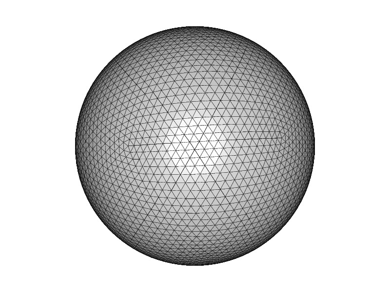
(a) Sphere

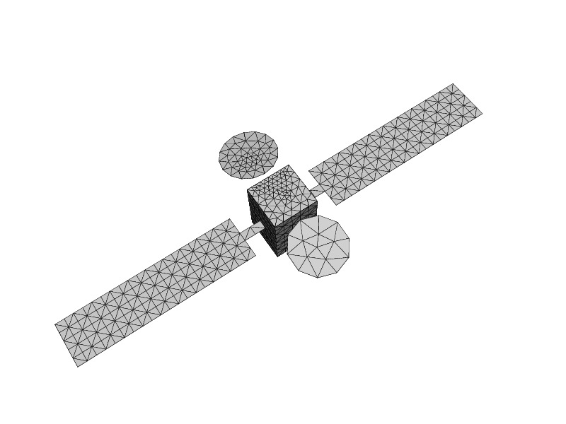
(b) Satellite

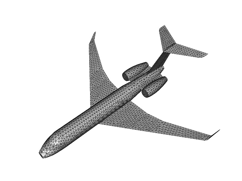
(c) Jet prototype

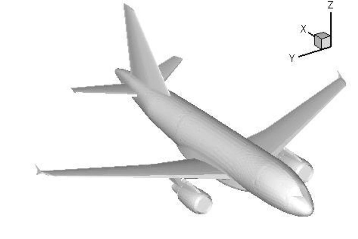
(d) Airbus A318 prototype

Figure 1: Meshes associated with test examples.

Example	Description	Size	Memory (Gb)	Frequency (MHz)	$\kappa_{1}(A)$	Geometry
1	Sphere	12000	4.6	535	$6\cdot\mathcal{O}(10^{5})$	Fig. 1(a)
2	Satellite	1699	0.1	57	$1\cdot\mathcal{O}(10^{5})$	Fig. 1(b)
3	Jet prototype	7924	2.0	615	$1\cdot\mathcal{O}(10^{7})$	Fig. 1(c)
4	Airbus A318 prototype	23676	18.0	800	$1\cdot\mathcal{O}(10^{7})$	Fig. 1(d)

Table 20: Characteristics of the model problems.

${\raise 2.71246pt\hbox{Solver}\!\mathord{\left/{\vphantom{{Solver}{Example}}}\right.\kern-1.2pt}\!\lower 2.71246pt\hbox{Example}}$	1	2
CORS	380 (211)	371 (11)
BiCOR	441 (251)	431 (15)
GMRES(50)	$>$ 3000 ($>$ 844)	871 (17)
QMR	615 (508)	452 (24)
TFQMR	399 (435)	373 (27)
BiCGSTAB	764 (418)	566 (18)

Table 21: Number of iterations and CPU time (in seconds) required by Krylov methods to reduce the initial residual to $\mathcal{O}(10^{-5})$.

${\raise 2.71246pt\hbox{Example}\!\mathord{\left/{\vphantom{{Solver}{Example}}}\right.\kern-1.2pt}\!\lower 2.71246pt\hbox{Solver}}$	CORS	GMRES(50)
3	1286 (981)	$>$3000 ($>$1147)
4	924 (5493)	2792 (8645)

Table 22: Number of iterations and CPU time (in seconds) for CORS and GMRES(50) to reduce the initial residual to $\mathcal{O}(10^{-3})$ on the two aircraft problems 1(c) and 1(d). These problems do not converge in 3000 iterations.

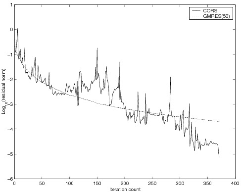
(a) On Example 2

Figure 2: Convergence histories for CORS and GMRES.

The large spectrum of real and complex linear systems, in both sparse and dense matrix computation, reported in this study illustrate the favourable numerical properties of the proposed unsymmetric variant of the Lanczos procedure for linear systems. The results indicate that our computational techniques are capable to solve very efficiently a large variety of problems. Therefore, they can be a suitable numerical tool to use in applications.

References

- [1] B. Carpentieri, I.S. Duff, L. Giraud, and G. Sylvand. Combining fast multipole techniques and an approximate inverse preconditioner for large electromagnetism calculations. SIAM J. Scientific Computing, 27(3):774–792, 2005.
- [2] T. Davis. Sparse matrix collection, 1994. http://www.cise.ufl.edu/research/sparse/matrices.
- [3] D. Day. An efficient implementation of the nonsymmetric lanczos algorithms. SIAM J. Matrix Anal. Appl., 18:566–589, 1997.
- [4] A. Edelman. The first annual large dense linear system survey. The SIGNUM Newsletter, 26:6–12, 1991.
- [5] A. Edelman. Large dense numerical linear algebra in 1993: The parallel computing influence. Journal of Supercomputing Applications., 7:113–128, 1993.
- [6] Ö. Ergül and L. Gürel. Fast and accurate solutions of extremely large integral-equation problems discretized with tens of millions of unknowns. Electron. Lett., 43(9):499–500, 2007.
- [7] Ö. Ergül and L. Gürel. Efficient parallelization of the multilevel fast multipole algorithm for the solution of large-scale scattering problems. IEEE Transactions on Antennas and Propagation, 56(8):2335–2345, 2008.
- [8] R. Barrett et al. Templates for the Solution of Linear Systems: Building Blocks for Iterative Methods. SIAM, 1995.
- [9] R. Freund, M.H. Gutknecht, and N. Nachtigal. An implementation of the look-ahead Lanczos algorithm for non-Hermitian matrices. SIAM J. Scientific Computing, 14:137–158, 1993.
- [10] R. W. Freund and N. M. Nachtigal. QMR: a quasi-minimal residual method for non-Hermitian linear systems. Numerische Mathematik, 60(3):315–339, 1991.
- [11] M.H. Gutknecht. Lanczos-type solvers for nonsymmetric linear systems of equations. Acta Numerica, 6:271–397, 1997.
- [12] Y.-F. Jing, T.-Z. Huang, Y. Zhang, L. Li, G.-H. Cheng, Z.-G. Ren, Y. Duan, T. Sogabe, and B. Carpentieri. Lanczos-type variants of the COCR method for complex nonsymmetric linear systems. Journal of Computational Physics, 228(17):6376–6394, 2009.
- [13] T. Malas, Ö. Ergül, and L. Gürel. Sequential and parallel preconditioners for large-scale integral-equation problems. In Computational Electromagnetics Workshop, August 30-31, 2007, Izmir, Turkey, pages 35–43, 2007.
- [14] T. Malas and L. Gürel. Incomplete LU preconditioning with multilevel fast multipole algorithm for electromagnetic scattering. SIAM J. Scientific Computing, 29(4):1476–1494, 2007.
- [15] B. Parlett. Reduction to tridiagonal form and minimal realizations. SIAM J. Matrix Analysis and Applications, 13:567–593, 1992.
- [16] B. Parlett, D. Taylor, and Z.-S. Liu. A look-ahead lanczos algorithm for unsymmetric matrices. Math. Comp., 44:105–124, 1985.
- [17] Y. Saad. A flexible inner-outer preconditioned GMRES algorithm. SIAM J. Scientific and Statistical Computing, 14:461–469, 1993.
- [18] Y. Saad. Iterative Methods for Sparse Linear Systems. PWS Publishing, New York, 1996.
- [19] Y. Saad and M.H. Schultz. GMRES: A generalized minimal residual algorithm for solving nonsymmetric linear systems. SIAM J. Scientific and Statistical Computing, 7:856–869, 1986.
- [20] V. Simoncini and D. B. Szyld. Recent computational developments in krylov subspace methods for linear systems. Numerical Linear Algebra with Applications, 14:1–59, 2007.
- [21] Gerard L. G. Sleijpen and Henk A. Van Der Vorst. An overview of approaches for the stable computation of hybrid bicg methods. Appl. Numer. Math., 19:235–254, 1995.
- [22] T. Sogabe. Extensions of the conjugate residual method. PhD thesis, University of Tokyo, 2006.
- [23] T. Sogabe, M. Sugihara, and S.-L. Zhang. An extension of the conjugate residual method to nonsymmetric linear systems. J. Comput. Appl. Math., 226:103– 113, 2009.
- [24] J.M. Song and W.C. Chew. The Fast Illinois Solver Code: Requirements and scaling properties. IEEE Computational Science and Engineering, 5(3):19–23, 1998.
- [25] J.M. Song, C.-C. Lu, and W.C. Chew. Multilevel fast multipole algorithm for electromagnetic scattering by large complex objects. IEEE Transactions on Antennas and Propagation, 45(10):1488–1493, 1997.
- [26] J.M. Song, C.C. Lu, W.C. Chew, and S.W. Lee. Fast illinois solver code (FISC). IEEE Antennas and Propagation Magazine, 40(3):27–34, 1998.
- [27] P. Sonneveld. CGS, a fast Lanczos-type solver for nonsymmetric linear systems. SIAM J. Scientific and Statistical Computing, 10:36–52, 1989.
- [28] G. Sylvand. La Méthode Multipôle Rapide en Electromagnétisme : Performances, Parallélisation, Applications. PhD thesis, Ecole Nationale des Ponts et Chaussées, 2002.
- [29] G. Sylvand. Complex industrial computations in electromagnetism using the fast multipole method. In G.C. Cohen, E. Heikkola, P. Joly, and P. Neittaanmdki, editors, Mathematical and Numerical Aspects of Wave Propagation, pages 657–662. Springer, 2003. Proceedings of Waves 2003.
- [30] H.A. van der Vorst. Bi-CGSTAB: a fast and smoothly converging variant of Bi-CG for the solution of nonsymmetric linear systems. SIAM J. Scientific and Statistical Computing, 13:631–644, 1992.