Transfer Matrices and Circuit Representation for the
Semiclassical Traces of the Baker Map

Abstract

Because of a formal equivalence with the partition function of an Ising chain, the semiclassical traces of the quantum baker map can be calculated using the transfer-matrix method. We analyze the transfer matrices associated with the baker map and the symmetry-reflected baker map (the latter happens to be unitary but the former is not). In both cases simple quantum-circuit representations are obtained, which exhibit the typical structure of qubit quantum bakers. In the case of the baker map it is shown that nonunitarity is restricted to a one-qubit operator (close to a Hadamard gate for some parameter values). In a suitable continuum limit we recover the already known infinite-dimensional transfer-operator. We devise truncation schemes allowing the calculation of long-time traces in regimes where the direct summation of Gutzwiller’s formula is impossible. Some aspects of the long-time divergence of the semiclassical traces are also discussed.

I Introduction

The quantum baker’s map balazs87 is a very useful test-bench for investigating quantum-classical correspondence issues in a variety of settings. Conceived as a model for studying the semiclassical limit of closed chaotic systems, it was first applied to analyze the random-matrix conjecture, the scarring phenomenon, Gutwiller’s trace formula and the long-time validity of semiclassical approximations (see, e.g., balazs89 ; saraceno90 ; ozorio91 ; saraceno94 ; dittes94 ; heller96 ). In the last years “open” quantum bakers were constructed and employed for studying semiclassical aspects of the scattering problem openbaker , e.g., the fractal Weyl law for the distribution of resonances schomerus04 .

The quantum baker also appeared in a variety of problems of Quantum Information, Quantum Computation and Quantum Open Systems. It was noted that the quantum baker could be efficiently realized in terms of quantum gates schack98 . A three qubit Nuclear Magnetic Resonance experiment was proposed brun99 and then implemented (with some simplifications) weinstein02 .

On the theoretical side, Schack and Caves schack00 showed that the Balazs-Voros-Saraceno quantum baker balazs89 ; saraceno90 can be seen as a shift on a string of quantum bits (in full analogy with the classical case), thus taking an important step towards generalizing the method of symbolic dynamics to the quantum case. At the same time, their circuit representation led naturally to a family of alternative quantizations. This family of bakers was the subject of several studies soklakov00 ; tracy02 ; scott03 . The ability of the baker family to generate entanglement was first studied by Scott and Caves scott03 (see also abreu06 ). Decoherent variants of the baker map were constructed by including mechanisms of dissipation and/or diffusion lozinski02 ; soklakov02 ; bianucci02 .

From the point of view of the structure of the quantum baker map, important results were recently obtained by Ermann and Saraceno ermann06 , who, building upon previous work by Lakshminarayan and Meenakshisundaram laksh05 , generalized the Schack-Caves family, and showed that all quantum bakers are perturbations of a common kernel (the “essential” baker).

The present paper focuses on an almost unexplored aspect of the semiclassical theory of the quantum baker map. Gutzwiller’s approximate formula for the traces of the baker map is formally equivalent to the partition function of a finite Ising chain (with exponentially decaying interactions and imaginary temperature). Thus, it can be evaluated with the standard transfer-matrix method. We have studied extensively the transfer matrices associated with the semiclassical traces of the baker map and the symmetry-reflected baker map. Our most remarkable finding is the existence of a qubit structure hidden in the semiclassical traces: the transfer matrices admit a quantum-circuit representation that is very similar to that found by Schack-Caves for the quantum baker.

We know of two studies of the baker map which applied the transfer matrix method (to the semiclassical long-time propagation of wave-packets heller96 , to the analysis of periodic-orbit action correlations smilansky03 ). Different in spirit, the present work aims at analyzing the transfer-matrix method in itself.

The paper is organized as follows. First we discuss the general structure of the transfer matrices for the baker map, exhibiting their quantum-circuit representation. Though the transfer matrices are not unitary, nonunitarity is restricted to a one-qubit “gate”. Except for this fact, the transfer matrices resemble qubit quantum bakers (Sec. II).

Section III is devoted to spectral properties. We show that all eigenvalues lie inside the unit circle in the complex plane, or very close to it. The number of eigenvalues close to the unit circle coincides approximately with the quantum dimension (for a suitable parameter range). This situation is very similar to that found in the infinite-dimensional transfer-operator method dittes94 ; tanner99 . Indeed we show that the transfer operator arises as a suitable continuum limit of the transfer matrix.

In Sec. IV we exhibit truncation schemes which permit the calculation of long-time traces.

Some aspects of the long-time divergence of the semiclassical traces are assessed in Sec. V.

The baker map possesses a spatial symmetry. If one is interested in separating the spectrum/traces into symmetry classes, then one must consider also the symmetry-related transfer matrices. Though similar to the matrices of Sec. II in many respects, these matrices happen to be exactly unitary. They are studied in Sec. VI.

Concluding remarks are presented in Sec. VII.

II Baker map: Transfer matrix

In order to make the paper self-contained we start by summarizing some basic information about the baker map.

The dynamics of the classical baker map is schematically depicted in Fig. 1.

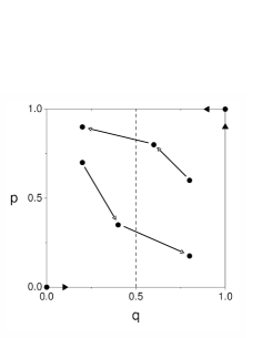
Figure 1: The classical baker map. The dynamics is controlled by the fixed points $(0,0)$ (for $q\leq 0.5$) and $(1,1)$ ($q>0.5$). The action of the map is to compress/stretch the coordinates $p/q$ relative to the fixed points by a factor of two. Some examples are depicted.

It acts on the unit square piecewise-linearly. Points with $q<0.5$ are governed by the hyperbolic point at the origin. If $q\geq 0.5$ the fixed point at $(1,1)$ rules. In any case the coordinates $p/q$ relative to the fixed point are compressed/stretched by a factor of two:

$$p^{\prime} = \frac{1}{2}\left(p+\epsilon\right)\,,$$ (1)

$$q^{\prime} = 2\,q-\epsilon\,,$$ (2)

where $\epsilon=[2q]$, the integer part of $2q$.

The quantum analogue of the classical mapping is a unitary operator acting on an even-dimensional Hilbert space balazs87 ; balazs89 . In the $q$-representation its matrix reads saraceno90 :

$$B=G_{N}^{-1}\left(\begin{array}[]{cc}G_{N/2}&0\\ 0&G_{N/2}\end{array}\right)\,,$$ (3)

where $G_{N}$ is the $N$-dimensional antiperiodic Fourier matrix:

$$(G_{N})_{mn}=\frac{1}{\sqrt{N}}\,e^{-2\pi i(n+1/2)(m+1/2)/N}\,,$$ (4)

with $0\leq m,n\leq N-1$. For this abstract system the Planck constant coincides with the inverse of the dimension, i.e., $\hbar=1/(2\pi N)$.

Our main concern are the traces of the quantum baker, ${\rm tr}\,B^{L}$, for $L=1,2,\ldots$. In the semiclassical regime of $N$ large enough (for a given $L$) the traces can be approximated by the Gutzwiller formula saraceno94

$${\rm tr}\,B^{L}\approx\frac{2^{L/2}}{2^{L}-1}\sum_{\epsilon}e^{2\pi iN{\cal S}(\epsilon)}~{},$$ (5)

where the sum runs over all periodic trajectories of length $L$ of the classical map, indexed by the binary column vectors $\epsilon=(\epsilon_{0},\epsilon_{1},\ldots,\epsilon_{L-1})^{t}$, with $\epsilon_{i}=0,1$. The corresponding actions ${\cal S}(\epsilon)$ are quadratic functions of the binary symbols,

$${\cal S}(\epsilon)=\epsilon^{t}A\,\epsilon\;.$$ (6)

The “coupling” matrix $A$ is suitably expressed in terms of the matrix $S$ of a cyclic shift, $S\cdot(a_{0},a_{1},\ldots a_{L-1})^{t}=(a_{1},\ldots,a_{L-1},a_{0})^{t}$ toscano97 :

$$A=\frac{2^{L-1}}{2^{L}-1}\sum_{i=0}^{L-1}\frac{S^{i}}{2^{i}}\;.$$ (7)

The trace formula for the baker map (5) can be derived as follows. Write ${\rm tr}\,B^{L}$ as a sum of products of Fourier matrix elements using Eq. (3). Approximate sums by integrals. Extend the limits of integration (which in principle are finite) to $\pm\infty$. The remaining integrals, being Gaussian, can be done exactly, giving the Gutzwiller sum saraceno94 .

Equation (5) is a particular case of the general Gutzwiller trace formula for systems with a chaotic classical limit. For such systems the trace formula lays a bridge between the quantum spectrum and the set of classical periodic orbits. It constitutes the core of all semiclassical schemes for relating energy levels to classical information, from the pioneer attempts gutzwiller82 ; gutzwiller , to the most recent, highly sophisticated developments haake .

The baker is very special in that all its periodic orbits, and properties thereof, are known analytically. So, in principle, the periodic-orbit sum (5) can be calculated for any $L$. However, because of the exponential growth of the number of periodic orbits with period, the brute-force summation is restricted to, say, $L\leq 30$. Remarkably, the method developed by Dittes, Doron and Smilansky dittes94 does not suffer from such a limitation. These authors defined an infinite-dimensional integral operator,

$$W(q^{\prime},q)=\frac{1}{\sqrt{2}}\left[\delta\left(q-\frac{q^{\prime}}{2}\right)+\delta\left(q-\frac{q^{\prime}+1}{2}\right)e^{2\pi iNq}\right]\,,$$ (8)

$0\leq q,q^{\prime}\leq 1$, whose traces give exactly the periodic-orbit sum of Eq. (5). They showed that ${\rm tr}\,W^{L}$ can be efficiently calculated from the eigenvalues of the matrix of $W$ in the Fourier basis, after suitable truncation dittes94 ; tanner99 .

An alternative to the infinite-dimensional operator method relies on the formal identification of the periodic-orbit sum (5) with the partition function of an Ising chain, for a purely imaginary temperature. The cyclical nature of the coupling matrix $A$ says that this is a circular chain, consisting of $L$ spins. All spins interact among themselves, but, as interactions decay exponentially with distance, one may expect some computational benefit (without much loss of accuracy) by truncating the interaction to some given number $r$ of closest neighbors, i.e.,

$$A\approx\frac{2^{L-1}}{2^{L}-1}\sum_{i=0}^{r}\frac{S^{i}}{2^{i}}\;.$$ (9)

The exact periodic-orbit sum corresponds to setting $r=L-1$ (no truncation at all), but, in principle, one can consider any truncation, even to first neighbors ($r=1$).

Once one has established the equivalence between the baker periodic-orbit sum and the Ising partition function, the transfer-matrix method can be invoked. The first-neighbor case is explained in textbooks reichl . It seems that the many-neighbor case has not been explicitly worked out in the literature, but some discussions exist hints ; gutzwiller . Anyway, even if not trivial, the generalization can be carried out following the spirit of the one-neighbor case and, in the case of the baker-Ising, leads to

$$\frac{2^{L/2}}{2^{L}-1}\sum_{\epsilon}e^{2\pi iN{\cal S}(\epsilon)}\approx\frac{2^{L}}{2^{L}-1}{\rm tr}\,M^{L}\,,$$ (10)

the explicit expression for $M$ being smilansky03 :

$$M=\frac{1}{\sqrt{2}}\left(\begin{array}[]{cccccccc}1&1&0&0&\cdots&\cdots&0&0\\ 0&0&1&1&0&\cdots&0&0\\ \vdots&\vdots&\vdots&\vdots&\vdots&\ddots&\vdots&\vdots\\ 0&0&0&0&\cdots&\cdots&1&1\\ a_{0}&a_{1}&0&0&\cdots&\cdots&0&0\\ 0&0&a_{2}&a_{3}&\cdots&\cdots&0&0\\ \vdots&\vdots&0&0&\cdots&\ddots&\vdots&\vdots\\ 0&\cdots&0&0&\cdots&\cdots&a_{2^{r}-2}&a_{2^{r}-1}\end{array}\right)\,.$$ (11)

The elements $a_{k}$ are given by

$$a_{k}=\exp\left[i\alpha\left(1+\frac{k}{2^{r}}\right)\right]\,,$$ (12)

with $0\leq k\leq 2^{r}-1$, and

$$\alpha=\frac{\pi N\,2^{L}}{2^{L}-1}\,.$$ (13)

Note that $M$ is a complex matrix depending on the three parameters $(N,L,r)$. Its dimension is $2^{r}\times 2^{r}$, with $r\leq L-1$. When $r=L-1$ one recovers the exact semiclassical traces, i.e., Eq. (10) becomes an equality.

A prefactor $1/\sqrt{2}$ has been absorbed into the definition of $M$ because in this way most of the spectrum of $M$ lies close to the unit circle or inside it (see Sec. III below). So, the transfer matrix $M$ becomes qualitatively similar to the semiclassical transfer operator of Refs. dittes94 ; tanner99 (we come back to this point later).

The transfer matrix approach transforms the calculation of the Gutzwiller sum into the problem of obtaining the trace of the $L$-th power of the finite matrix $M$. From a numerical point of view this is advantageous only if truncation of $M$ is admissible. We defer the analysis of this question until Sec. V. Now we concentrate on the transfer matrices themselves which, as we shall show, possess very interesting properties.

The transfer matrix (11) exhibits the structure of a tensor product which is conveniently displayed by switching to a qubit representation. This consists in identifying the “spatial” degree of freedom $q$ with the tensor product of $r$ two-level systems:

$$|k\rangle\equiv|\epsilon_{0}\rangle\otimes|\epsilon_{1}\rangle\otimes\ldots\otimes|\epsilon_{r-1}\rangle\,.$$ (14)

Here $k$ indexes the states of the $q$-basis and $\epsilon_{i}=0,1$ is a label for the qubit basis states; they are related through the binary expansion

$$k=\epsilon_{0}+2\epsilon_{1}+\ldots 2^{r-1}\epsilon_{r-1}\,.$$ (15)

In the qubit picture the matrix $M$ can be broken up into the elementary gates shown in the quantum circuit of Fig. 2.

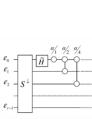
Figure 2: Quantum circuit associated with the semiclassical trace of the $L$-th power of the baker map. The parameter $r\leq L-1$ controls the level of truncation ($r=L-1$ corresponds to no truncation at all). From left to right, the circuit is composed of a downwards shift of all qubits $(S^{\downarrow})$, a nonunitary one-qubit gate $\tilde{H}$, and a sequence of symmetric phase gates.

The circuit acts on $r$ qubits, starting with a downwards cyclic shift of all qubits, i.e.,

$$S^{\downarrow}|\epsilon_{0}\rangle\otimes|\epsilon_{1}\rangle\otimes\ldots\otimes|\epsilon_{r-1}\rangle=|\epsilon_{r-1}\rangle\otimes|\epsilon_{0}\rangle\otimes|\epsilon_{1}\rangle\otimes\ldots\otimes|\epsilon_{r-2}\rangle\;.$$ (16)

A nonunitary gate acting on the first qubit follows, which bears some resemblance with a Hadamard gate,

$$\tilde{H}=\frac{1}{\sqrt{2}}\left(\begin{array}[]{cc}1&1\\ 1&x\end{array}\right)\,,$$ (17)

with

$$x=\exp\left(\frac{2\pi iN}{2^{L}-1}\right)\,.$$ (18)

It must be noted that, as the dimension $N$ is an even number, we always have $x\neq-1$, and $\tilde{H}$ is never unitary. After the $\tilde{H}$ gate one finds a single qubit phase gate,

$$P_{00}(\alpha)=\left(\begin{array}[]{cc}1&0\\ 0&{\mbox{e}}^{i\alpha}\end{array}\right)\,.$$ (19)

Finally one has a sequence of two-qubit phase gates, acting symmetrically between the first and the $k$-th qubit,

$$P_{0k}(\beta)=\left(\begin{array}[]{cccc}1&0&0&0\\ 0&1&0&0\\ 0&0&1&0\\ 0&0&0&{\mbox{e}}^{i\beta}\end{array}\right)\,,$$ (20)

with exponentially decreasing phases, $\beta=\alpha/2,\alpha/4,\ldots,\alpha/2^{r}$.

Writing $M$ as a circuit has helped us in identifying its basic constituents. In particular we recognize the one-qubit gate $\tilde{H}$ as responsible for the deviation from unitarity. If we substitute $\tilde{H}$ by a Hadamard gate, i.e., set $x=-1$ in (17), then the circuit of Fig. 2 acquires the typical structure of the baker family ermann06 : an “essential-baker” block (formed by a shift $S^{\downarrow}$ and a single-qubit Fourier transform) followed by a “diffraction kernel” (phase gates).

III Spectral Properties

Figure 3 displays a typical transfer-matrix spectrum in the case that the dimension of the transfer matrix is much larger than the quantum dimension, i.e., $2^{L-1}\gg N$.

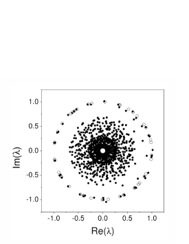
Figure 3: Comparison of spectra. Open circles correspond to the quantum baker map ($N=46$) and dots to the semiclassical transfer matrix for $L=11$.

The spectrum can be coarsely divided into three parts. Approximately $N$ eigenvalues are localized close to the unit circle. Most of the remaining ones are concentrated in a disk of smaller radius, and there are some transitional eigenvalues spiraling out from the inner disk to the unit circle. The eigenvalues lying close to the unit circle can be put in almost one-to-one correspondence with the exact eigenvalues of the quantum baker (3).

Increasing $L$ while keeping $N$ fixed does not significantly change the almost unitary part of spectrum, but populates the region of small moduli (see Fig. 4).

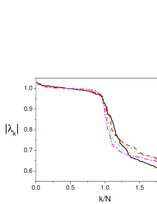
Figure 4: (color online) Semiclassical eigenvalues (moduli) versus scaled eigenvalue index $k/N$ (decreasing order). Note the clear transition around $k/N=1$. Parameters are $N=82$ and $L=9,10,11,12$ (black/solid, red/dash, green/dot, magenta/dash-dot, respectively).

This fact, when combined with the existence of eigenvalues with moduli larger than one, leads to the conclusion that Gutzwiller’s traces for the baker are divergent in the limit $L\to\infty$ (fixed $N$). This result has been confirmed previously using the transfer-operator method argaman93; dittes94 ; tanner99 .

Indeed, the overall features of the transfer-matrix spectrum described above can also be found in the transfer-operator spectra discussed in Refs. dittes94 ; tanner99 . Looking for an explanation for this similarity, we recall that the transfer operator is infinite-dimensional and independent of $L$. Thus, one may be tempted to compare Eq. (8) with the infinite-$L$ limit of the transfer matrix (11). In this limit, the transfer matrix becomes an integral kernel, indices becoming continuous variables:

$$\frac{k}{2^{r}-1}\to q\,,\qquad 0\leq q\leq 1\,.$$ (21)

A careful calculation verifies that the transfer matrix tends to the transfer operator, i.e.,

$$\lim_{L\to\infty}M_{kk^{\prime}}=W(q,q^{\prime})\,,$$ (22)

with $W(q,q^{\prime})$ precisely that given in Eq. (8)! So, the transfer operator is formally recovered as the continuum limit of the transfer matrix.

IV Truncation Schemes

Here we discuss the numerical calculation of long-time Gutzwiller traces using the transfer-matrix formula (10). The most natural procedure for calculating ${\rm tr}M^{L}$ requires the diagonalization of $M$ to obtain its eigenvalues. This scheme is limited to very small values of $L$, e.g., to $L\lesssim 15$ in a personal computer. So, truncation becomes essential.

The error introduced in truncating the interactions to $r$ neighbors can be roughly estimated from Eq. (9) and the basic definitions (5,6,7). Such a truncation produces an error in the actions (6) approximately given by

$$\delta{\cal S}\sim\frac{1}{2}\,\epsilon^{t}\,\frac{S^{r}}{2^{r}}\,\epsilon\;.$$ (23)

For typical vectors $\epsilon$, containing randomly distributed 0/1 bits, we have

$$\epsilon^{t}\,S^{r}\,\epsilon\sim\frac{L}{4}\,.$$ (24)

This implies that the corresponding error in the Gutzwiller phases amounts to

$$\delta\phi\equiv\delta\left(2\pi N{\cal S}\right)\sim\frac{NL}{2^{r}}\;.$$ (25)

Finally, if we assume that this is the error committed in most phases in the Gutzwiller sum (5), then $\delta\phi$ amounts to the relative error in the semiclassical traces, for

$$\delta\sum e^{i\phi_{k}}=\sum e^{i\phi_{k}}\delta\phi_{k}\approx\delta\phi\sum e^{i\phi_{k}}\;.$$ (26)

Thus, we arrive at the following condition for the validity of the truncation to $r$ neighbors:

$$\frac{2^{r}}{NL}\equiv f\gg 1\,.$$ (27)

However, even after truncating the transfer matrix, we may need to use values of $r$ which make diagonalization prohibitive, e.g., for $N=50$, $L=1000$. Remarkably there is an alternative to diagonalization which arises from the sparsity of $M$. For, even if the special type of sparsity $M$ exhibits is not helpful in speeding-up its diagonalization, it permits us to implement an alternative, much more efficient method for calculating the traces of $M$.

Consider the following identity:

$${\rm tr}M_{r}^{L}=2^{r}\,\overline{\langle\psi\left|M_{r}^{L}\right|\psi\rangle}\,,$$ (28)

where overline means average over random complex vectors $|\psi\rangle$ uniformly distributed over the corresponding unit sphere mehta . (The notation $M_{r}$ has been used to indicate the truncation of $M$ to $r$ qubits.) The idea behind (28) is to calculate $\langle\psi|M_{r}^{L}|\psi\rangle$ by applying iteratively the matrix $M_{r}$ to $|\psi\rangle$, and then averaging over $|\psi\rangle$. This method allows one, in principle, to consider $r$ as large as 20.

Table 1 displays some examples.

	$\;L\;$	$\;\;r\;\;$	TMM	TOM	exact
a	20	10	$\;3.73[5]$	$\;3.87[6]$	3.85
b	20	11	$\;3.90[7]$	$\;3.87[6]$	3.85
c	20	12	$\;3.85[3]$	$\;3.87[6]$	3.85
d	20	13	$\;3.84[5]$	$\;3.87[6]$	3.85
e	20	14	$\;3.89[5]$	$\;3.87[6]$	3.85
f	40	13	$\;2.04[2]10^{1}$	$\;1.99[1]10^{1}$	?
g	60	13	$\;1.00[5]10^{1}$	$\;1.05[5]10^{1}$	?
h	80	13	$\;1.30[2]10^{2}$	$\;1.24[1]10^{2}$	?
i	160	13	$\;1.00[1]10^{4}$	$\;9.0[3]10^{3}$	?

Table 1: Gutzwiller’s traces (absolute value). We compare the transfer-matrix method (TMM) with the transfer-operator method (TOM) and exact results. In all cases the quantum dimension is $N=24$. The square brackets contain the estimated error in the least significative figure [e.g., the notation $1.30[2]10^{2}$ stands for $(1.30\pm 0.02)\times 10^{2}$]. The values in the TMM column are the result of averaging over more than $10^{5}$ random states; the errors are statistical. In the TOM case the errors correspond to the variation of the results when the size of the Fourier basis is varied from 149 to 201 dittes94 ; tanner99 .

The first rows (a-e) illustrate the improvement of the results as the truncation level $r$ is increased, for fixed $(N,L)$. Agreement with the exact results is met, within the specified statistical errors, for $r\geq 12$, corresponding to $f\gtrsim 4$. In rows (f-i) we consider $(N,r)$ fixed and large values of $L$ which can in no way be reached by direct computation of the periodic orbit summation, so that exact results are not known for such $L$. In these cases we compare with the approximate results obtained using the transfer-operator method dittes94 ; tanner99 .

We see good agreement for $L\lesssim 80$, i.e., we find the condition $f\gtrsim 4$ again.

So, we have checked that the transfer-matrix method works satisfactorily in the parameter regime specified by (27).

V Divergence of long-time traces

For chaotic systems, the Gutzwiller trace formula is only the first term of an expansion in powers of $\hbar$. Because of this, the semiclassical eigenvalues obtained from the Gutwiller traces deviate in general from the unit circle in the complex plane. For typical chaotic systems it is expected that the distance of the largest semiclassical eigenvalue to the unit circle scales like $\hbar$, i.e., $1/N$ for quantum maps keating94 . In the case of the baker map, an anomalous behavior $N^{-1/2}$ is observed which is due to diffraction effects originating in the discontinuities of the mapping dittes94 ; tanner99 . In any case, this lack of unitarity makes Gutzwiller’s traces exponentially growing with $L$, a behavior that may be guessed from Table 1.

The following question arises naturally: can the $N^{-1/2}$ law be associated with the particular structure of the baker transfer matrix? In the circuit representation (Fig. 2) nonunitarity arises from the single-qubit gate $\tilde{H}$. So, one may ask: what is typically the largest eigenvalue (in modulus) of a map obtained by tensoring $\tilde{H}$ with a generic $N$-dimensional unitary gate $U$?

On the other side, the $q$-representation (11) offers a different point of view of the nonunitarity: the transfer matrix can be split as $M=(U_{1}+U_{2})/\sqrt{2}$, with $U_{i}$ unitary matrices of dimension $N$ [see Eq. (31)]. How does the leading eigenvalue of such a matrix $M$ scale with $N$?

In order to answer the questions above we resorted to numerical calculations. First we analyzed the matrices $H^{\prime}\otimes U$ with $U$ a random matrix belonging to the Circular Unitary Ensemble (CUE). The matrix $H^{\prime}$ acts on the least significant qubit and is defined by Eq. (17) with $x=1$, i.e., $H^{\prime}$ is chosen to be the large-$L$ limit of $\tilde{H}$. Then we considered the ensemble $(U_{1}+U_{2})/\sqrt{2}$ with $U_{i}$ independent random matrices belonging to CUE gorlich04 . In order to check any possible ensemble dependence we also calculated the case $H^{\prime}\otimes U$ with $U$ in the Circular Orthogonal Ensemble (COE).

Our results are exhibited in Fig. 5.

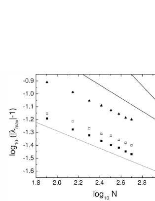
Figure 5: Average distance of the largest eigenvalue to the unit circle versus dimension for three ensembles of nonunitary random matrices. Triangles, squares, and circles correspond to $H^{\prime}\otimes\rm{COE}$, $(\rm{CUE}+\rm{CUE})/\sqrt{2}$ (normalized sum of two independent CUE matrices), and $H^{\prime}\otimes\rm{CUE}$, respectively. See text for the definition of the single-qubit nonunitary gate $H^{\prime}$. Error bars correspond to statistical errors. Straight lines representing decay laws $N^{-1/3}$, $N^{-1/2}$, and $N^{-1}$ have been drawn for reference.

In the three considered cases we observe very similar decay laws. These decays are much closer to the diffractive scaling $N^{-1/2}$ than to the universal semiclassical behavior $N^{-1}$, meaning that the random-matrix modeling has partially captured the essence of the semiclassical baker. However, there is still some noticeable departure from the $N^{-1/2}$ decay (rather, our numerical results seem to follow a $N^{-1/3}$ law). Thus, we conclude that the minimum-information models we have constructed still have to be complemented with some ingredient to properly describe the $N^{-1/2}$ baker scaling. Further research is necessary to discover what such an additional information should be (e.g., some particular correlation between $U_{1}$ and $U_{2}$?).

VI Reflected baker map

The quantum baker map $B$ is invariant under the parity symmetry $R$, its action on the $q$-basis being just $R\,|k\rangle=|N-k\rangle$. This is the quantum counterpart of the classical reflection symmetry ${\cal R}:(q,p)\rightarrow(1-q,1-p)$. When analyzing spectral properties it is convenient to separate eigenstates and eigenvalues of $B$ according to their parity. Thus, one is led to consider the parity-projected bakers $B_{\pm}=(B\pm BR)/2$. In the semiclassical domain the traces of $B_{\pm}$ can be approximated by saraceno94

$${\rm tr}\;B^{L}_{\pm}\approx\frac{1}{2}\,\,\left(\frac{2^{L/2}}{2^{L}-1}\sum_{\epsilon}e^{2\pi iNS(\epsilon)}~{}\pm~{}\\ \frac{2^{L/2}}{2^{L}+1}\sum_{\epsilon}e^{2\pi iNS^{\prime}(\epsilon)}\right)\,.$$ (29)

The first summation above correspond to the baker traces (5). In the second sum $S^{\prime}(\epsilon)$ stands for half the action [Eq. (6)] of a periodic orbit of length $2L$ with symbolic code $\epsilon=(\epsilon_{0},\epsilon_{1},\ldots,\epsilon_{L-1},\bar{\epsilon_{0}},\bar{\epsilon_{1}},\ldots,\bar{\epsilon_{L-1}})^{t}$, where $\bar{\epsilon_{i}}=1-\epsilon_{i}$. These are precisely the orbits invariant under the parity transformation.

We shall exhibit the transfer matrix associated to the reflected traces, pointing out the most important features. Following the same procedure as in Sec. II we constructed a transfer matrix $M^{\prime}$ such that

$$\sum_{\epsilon}e^{2\pi iNS^{\prime}(\epsilon)}={\rm tr}M^{\prime\,2L}\,.$$ (30)

After eliminating the null subspace that appears as a consequence of considering just the parity-invariant trajectories of length $2L$, the matrix $M^{\prime}$ is reduced to dimension $2^{L}\times 2^{L}$:

$$M^{\prime}=\left(\begin{array}[]{cccccccc}0&1&0&0&\cdots&\cdots&0&0\\ 0&0&0&1&0&\cdots&0&0\\ \vdots&\vdots&\vdots&\vdots&\vdots&\ddots&\vdots&\vdots\\ 0&0&0&0&\cdots&\cdots&0&1\\ a_{0}&0&0&0&\cdots&\cdots&0&0\\ 0&0&a_{1}&0&\cdots&\cdots&0&0\\ \vdots&\vdots&0&0&\cdots&\ddots&\vdots&\vdots\\ 0&\cdots&0&0&\cdots&\cdots&a_{2^{L-1}-1}&0\end{array}\right)\,,$$ (31)

where the matrix elements $a_{k}$ are given by

$$a_{k}=\exp\left[i\alpha^{\prime}\left(1+\frac{\tilde{k}}{2^{2L-1}}\right)\right]\,,$$ (32)

with

$$\alpha^{\prime}=\frac{\pi N\,2^{2L-1}}{2^{2L}-1}\,.$$ (33)

The last undefined ingredient is the integer $\tilde{k}$. It is best expressed in terms of the binary digits of the integer $k$ [see Eq. (15)]. If $k=\epsilon_{2^{L-1}-1}\ldots\epsilon_{1}\epsilon_{0}$, then

$$\tilde{k}=\epsilon_{2^{L-1}-1}\ldots\epsilon_{1}\epsilon_{0}\,0\,\overline{\epsilon_{2^{L-1}-1}}\ldots\bar{\epsilon_{1}}\bar{\epsilon_{0}}\,.$$ (34)

The main difference between the baker’s transfer matrix (11) and the matrix above, is that $M^{\prime}$ is exactly unitary (thus, its spectrum lies on the unit circle). Except for this fact, both $M$ and $M^{\prime}$ are structurally very similar. Perhaps this can be better appreciated by looking at the quantum circuit for $M^{\prime}$ in Fig. 6.

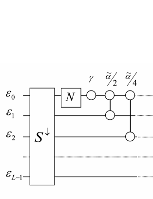
Figure 6: Quantum circuit associated with the semiclassical traces of the parity-reflected baker map. From left to right, the circuit is composed of a downwards shift of all qubits $(S^{\downarrow})$, a NOT gate ($N$), a one-qubit gate, and a sequence of $L-1$ two qubit phase gates. All gates are unitary.

The circuit acts on $L$ qubits (without truncation). It starts like the baker’s, with a downwards shift of all qubits. Then we have a NOT gate acting on the first qubit given by

$$N=\left(\begin{array}[]{cc}0&1\\ 1&0\end{array}\right)\,.$$ (35)

A phase gate $P_{00}(\gamma)$ follows that acts on the first qubit, with

$$\gamma=\alpha^{\prime}\left(1+\frac{2^{L-1}-1}{2^{2L-1}}\right)\,.$$ (36)

Finally there is a sequence of $L-1$ symmetrical two-qubit phase gates $P_{0k}(\beta)$ acting between the first and the $k$-th qubit with exponentially decreasing phases, $\beta=\tilde{\alpha}/2,\tilde{\alpha}/4,\ldots,\tilde{\alpha}/2^{L}$, where $\tilde{\alpha}=\alpha^{\prime}(2^{L}-1)/2^{L}$.

A complete study of the spectral properties of the reflected-baker transfer matrix, truncation schemes, etc, is deferred to a future publication because, as $M^{\prime}$ is unitary, such analyses would take us in directions very different than those followed in the case of the baker map. However, we would like to anticipate one result which gives a hint about the nature of the spectrum of $M^{\prime}$.

Consider the $2L$-th power of the transfer matrix $M^{\prime}$, i.e., the $2L$-th iteration of the circuit above. We verified that the shifts and NOT gates cancel out and only phase gates remain. This means that $M^{\prime\,2L}$ is a diagonal matrix (given that the phase gates are diagonal). It turns out that the diagonal elements are exactly the Gutwiller phases $\exp(iS^{\prime}/\hbar)$ in Eq. (29) (we tested this numerically for some cases). Thus, the spectrum of $M^{\prime}$ is formed by roots of the Gutzwiller phases!

VII Conclusions

We presented a study of the transfer matrix approach to the semiclassical traces of the baker map and its reflected version. We found that the transfer matrices admit a tensor product decomposition leading to simple circuit representations, similar to those obtained by Schack and Caves for the quantum baker. Remarkably, in the case of the baker, the corresponding circuit clearly isolates the source of nonunitarity of the semiclassical traces in the form of a one-qubit Hadamard-like gate. Given that both exact and semiclassical bakers can now be written as circuits, this representation appears as a promising tool for studying the corrections to the Gutzwiller trace formula.

In the case of the baker, spectral properties were analyzed, showing that there exists a close similitude with the transfer operator of Ref. dittes94 . In fact, we proved that the transfer operator arises as a suitable asymptotic limit of the transfer matrix formalism. Truncation schemes were discussed which permit the numerical calculation of long-time traces well inside a domain where direct summation of the Gutzwiller formula is impossible.

We would like to conclude by mentioning a very exciting (though rather speculative) possibility. It is tempting to think of the transfer matrices as maps for which the Gutzwiller formula is exact. Admittedly this point of view has some limitations because there is a map for each value of $L$. Even so, our results suggest that we may be not far from finding a close relative to the baker map having an exact periodic-orbit trace formula. The search for such a map constitutes a very attractive and challenging project which, however, exceeds the scope of the present paper.

References

- (1) N. L. Balazs and A. Voros, Europhys. Lett. 4, 1089 (1987).
- (2) N. L. Balazs and A. Voros, Ann. Phys. 190, 1 (1989).
- (3) M. Saraceno, Ann. Phys. 199, 37 (1990).
- (4) A. M. Ozorio de Almeida and M. Saraceno, Ann. Phys. 210, 1 (1991).
- (5) M. Saraceno and A. Voros, Physica D 79, 206 (1994).
- (6) F.-M. Dittes, E. Doron, and U. Smilansky, Phys. Rev. E 49, 963 (1994).
- (7) L. Kaplan and E. J. Heller, Phys. Rev. Lett. 76, 1453 (1996).
- (8) L. Ermann, G. G. Carlo, and M. Saraceno, Phys. Rev. Lett. 103, 054102 (2009); S. Nonnenmacher and M. Rubin, Nonlinearity 20, 1387 (2007); S. Nonnenmacher and M. Zworski, J. Phys. A 38, 10 683 (2005); J. P. Keating, M. Novaes, S. D. Prado, and M. Sieber, Phys. Rev. Lett. 97, 150406 (2006); J. P. Keating, S. Nonnenmacher, M. Novaes, and M. Sieber, Nonlinearity 21, 2591 (2008); M. Saraceno and R. O. Vallejos, Chaos 6, 193 (1996).
- (9) J. Sjöstrand, Duke Mathematica Journal 60, 1 (1990); H. Schomerus and J. Tworzydlo, Phys. Rev. Lett. 93, 154102 (2004).
- (10) R. Schack, Phys. Rev. A 57, 1634 (1998).
- (11) A. T. Brun and R. Schack, Phys. Rev. A 59, 2649 (1999)
- (12) Y. S. Weinstein, S. Lloyd, J. Emerson, and D. G. Cory, Phys. Rev. Lett. 89, 284102 (2002).
- (13) R. Schack and C. M. Caves, Appl. Algebra Eng. Commun. Comput. 10, 305 (2000).
- (14) A. N. Soklakov and R. Schack, Phys. Rev. E 61, 5108 (2000).
- (15) M. M. Tracy and A. J. Scott, J. Phys. A 35, 8341 (2002).
- (16) A. J. Scott and C. M. Caves, J. Phys. A 36, 9553 (2003).
- (17) R. F. Abreu and R. O. Vallejos, Phys. Rev. A 73, 052327 (2006).
- (18) A. N. Soklakov and R. Schack, Phys. Rev. E 66, 036212 (2002).
- (19) A. Lozinski, P. Pakonski, and K. Zyczkowski, Phys. Rev. E 66, 065201 (2002).
- (20) P. Bianucci, J. P. Paz, M. Saraceno, Phys. Rev. E 65, 046226 (2002).
- (21) L. Ermann and M. Saraceno, Phys. Rev. E 74, 046205 (2006).
- (22) A. Lakshminarayan, J. Phys. A 38, L597 (2005); N. Meenakshisundaram and A. Lakshminarayan, Phys. Rev. E 71, 065303(R) (2005).
- (23) U. Smilansky and B. Verdene, J. Phys. A: Math. Gen. 36, 3525 (2003).
- (24) G. Tanner, J. Phys. A: Math. Gen. 32, 5071 (1999).
- (25) F. Toscano, R. O. Vallejos and M. Saraceno, Nonlinearity 10, 965 (1997).
- (26) M. C. Gutzwiller, Physica D 5, 183 (1982).
- (27) M. C. Gutzwiller, Chaos in Classical and Quantum Mechanics (Springer, New York, 1990).
- (28) F. Haake, Quantum Signatures of Chaos (Springer-Verlag, Berlin, 2010).
- (29) L. E. Reichl, A Modern Course in Statistical Physics (John Wiley & Sons, Inc., New York, 1998).
- (30) J. F. Dobson, J. Math. Phys. 10, 40 (1969); C. Borzi, G. Ord, and J. K. Percus, J. Stat. Phys. 46, 51 (1987).
- (31) M. L. Mehta, Random Matrices (Elsevier, Amsterdam, 2004).
- (32) J. P. Keating, J. Phys. A: Math. Gen. 27 6605 (1994).
- (33) A. Görlich and A. Jarosz, arXiv:math-ph/0408019v2.