Bidifferential Calculus Approach to AKNS Hierarchies and Their Solutions

Bidifferential Calculus Approach
to AKNS Hierarchies and Their Solutions

Aristophanes DIMAKIS ^† and Folkert MÜLLER-HOISSEN ^‡

A. Dimakis and F. Müller-Hoissen

^† Department of Financial and Management Engineering, University of the Aegean,
^† 41, Kountourioti Str., GR-82100 Chios, Greece dimakis@aegean.gr

^‡ Max-Planck-Institute for Dynamics and Self-Organization,
^‡ Bunsenstrasse 10, D-37073 Göttingen, Germany folkert.mueller-hoissen@ds.mpg.de

Received April 12, 2010, in final form June 21, 2010; Published online July 16, 2010

We express AKNS hierarchies, admitting reductions to matrix NLS and matrix mKdV hierarchies, in terms of a bidifferential graded algebra. Application of a universal result in this framework quickly generates an infinite family of exact solutions, including e.g. the matrix solitons in the focusing NLS case. Exploiting a general Miura transformation, we recover the generalized Heisenberg magnet hierarchy and establish a corresponding solution formula for it. Simply by exchanging the roles of the two derivations of the bidifferential graded algebra, we recover “negative flows”, leading to an extension of the respective hierarchy. In this way we also meet a matrix and vector version of the short pulse equation and also the sine-Gordon equation. For these equations corresponding solution formulas are also derived. In all these cases the solutions are parametrized in terms of matrix data that have to satisfy a certain Sylvester equation.

AKNS hierarchy; negative flows; Miura transformation; bidifferential graded algebra; Heisenberg magnet; mKdV; NLS; sine-Gordon; vector short pulse equation; matrix solitons

37J35; 37K10; 16E45

1 Introduction

A unification of some integrability aspects and solution generating techniques has recently been achieved for a wide class of “integrable” partial differential or difference equations (PDEs) in the framework of bidifferential graded algebras [2]. The hurdle to take is to find a bidifferential calculus (i.e. bidifferential graded algebra) associated with the respective PDE. In particular, a surprisingly simple result (Theorem 3.1 in [2] and Theorem 3.3 below) then generates a (typically large) class of exact solutions. This has been elaborated in detail for matrix NLS systems in a recent work [3]. The present work extends some of these results to a corresponding hierarchy and moreover to related hierarchies. It demonstrates how to deal with whole hierarchies instead of only single equations or systems in the bidifferential calculus approach and shows moreover that certain relations between hierarchies find a nice explanation in this framework. Except for certain specializations, we deal with “non-commutative equations”, i.e. we treat the dependent variables as non-commutative matrices, and the solution formulas that we present respect this fact.

In Section 2 we introduce some basic structures needed in the sequel. Section 3 presents a bidifferential calculus for a matrix AKNS hierarchy. We derive a class of solutions of the latter and address some reductions of the hierarchy. In Sections 4 and 5 we show that, in the bidifferential calculus framework, a “reciprocal” [4] or “negative” extension of the hierarchy naturally appears. “Negative flows” have been considered previously via negative powers of a recursion operator (see e.g. [5, 6, 7, 8] and also [9, 10, 11, 12] for other aspects). In our picture, these rather emerge as “mixed equations”, bridging between the ordinary hierarchy and a “purely negative” counterpart.

Section 6 elaborates this program for a “dual hierarchy”. Here we recover in the bidifferential calculus framework in particular a well-known duality or gauge equivalence between the (matrix) NLS and (generalized) Heisenberg magnet hierarchies [13, 14, 15, 16, 17, 18, 19, 20]. Section 7 contains some concluding remarks.

2 Basic structures

Definition 2.1.

A graded algebra is an associative algebra $\Omega$ over $\mathbb{C}$ with a direct sum decomposition

$$\Omega=\bigoplus_{r\geq 0}\Omega^{r}$$

into a subalgebra $\mathcal{A}=\Omega^{0}$ and $\mathcal{A}$-bimodules $\Omega^{r}$, such that

$$\Omega^{r}\Omega^{s}\subseteq\Omega^{r+s}.$$

Definition 2.2.

A bidifferential calculus (or bidifferential graded algebra) is a graded algebra $\Omega$ equipped with two ($\mathbb{C}$-linear) graded derivations $\mathrm{d},\bar{\mathrm{d}}:\Omega\rightarrow\Omega$ of degree one (hence $\mathrm{d}\Omega^{r}\subseteq\Omega^{r+1}$, $\bar{\mathrm{d}}\Omega^{r}\subseteq\Omega^{r+1}$), with the properties

$$\mathrm{d}\circ\mathrm{d}=0,\qquad\bar{\mathrm{d}}\circ\bar{\mathrm{d}}=0,\qquad\mathrm{d}\circ\bar{\mathrm{d}}+\bar{\mathrm{d}}\circ\mathrm{d}=0,$$

and the graded Leibniz rule

$$\mathrm{d}(\chi\chi^{\prime})=(\mathrm{d}\chi)\chi^{\prime}+(-1)^{r}\chi\mathrm{d}\chi^{\prime},\qquad\bar{\mathrm{d}}(\chi\chi^{\prime})=(\bar{\mathrm{d}}\chi)\chi^{\prime}+(-1)^{r}\chi\bar{\mathrm{d}}\chi^{\prime},$$

for all $\chi\in\Omega^{r}$ and $\chi^{\prime}\in\Omega$.

For any algebra $\mathcal{A}$, a corresponding graded algebra is given by

$$\Omega=\mathcal{A}\otimes\bigwedge\big{(}\mathbb{C}^{N}\big{)},$$ (2.1)

where $\bigwedge(\mathbb{C}^{N})$ denotes the exterior algebra of $\mathbb{C}^{N}$, $N>1$. Defining graded derivations $\mathrm{d}$, $\bar{\mathrm{d}}$ on $\mathcal{A}$, they extend in an obvious way to $\Omega$ such that the Leibniz rule holds and elements of $\bigwedge(\mathbb{C}^{N})$ are treated as constants with respect to $\mathrm{d}$ and $\bar{\mathrm{d}}$.

Given a bidifferential calculus, it turns out that the equation

$$\bar{\mathrm{d}}\mathrm{d}\phi=\mathrm{d}\phi\wedge\mathrm{d}\phi,\qquad\mbox{where}\quad\phi\in\mathcal{A},$$ (2.2)

has various integrability properties [2, 3]. By choosing a suitable bidifferential calculus, this equation covers in particular the familiar selfdual Yang–Mills equation (in one of its gauge-reduced potential versions), but also e.g. discrete integrable equations [2, 3]. In the next section we demonstrate that, by choosing an appropriate bidifferential calculus, (2.2) reproduces matrix AKNS hierarchies.

The (modified) Miura transformation

$$[\bar{\mathrm{d}}g-(\mathrm{d}g)\Delta]g^{-1}=\mathrm{d}\phi,$$ (2.3)

where $\bar{\mathrm{d}}\Delta=(\mathrm{d}\Delta)\Delta$, is a hetero-Bäcklund transformation between (2.2) and the dual equation

$$\mathrm{d}\left([\bar{\mathrm{d}}g-(\mathrm{d}g)\Delta]g^{-1}\right)=0.$$ (2.4)

In the present work we concentrate on the case where $\Delta=0$. We note that (2.3) and (2.4) are equivalent if $\mathrm{d}$ has trivial cohomology. But this is in general not the case.

Exchanging $\mathrm{d}$ and $\bar{\mathrm{d}}$ in (2.2), we get a different equation. Dealing with hierarchies, such an exchange leads to what we call the reciprocal hierarchy. If $\Delta=0$, exchanging $\mathrm{d}$ and $\bar{\mathrm{d}}$ in (2.4), simply amounts to replacing $g$ by $g^{-1}$.

3 AKNS hierarchies

Let $\mathcal{B}_{0}$ be the algebra of complex smooth functions of independent variables $t_{1},t_{2},t_{3},\ldots$, $\mathcal{B}$ an extension by certain operators (specified below), and $\mathcal{A}=\mathrm{Mat}(m,m,\mathcal{B})$, $m>1$. Let $m=m_{1}+m_{2}$ with $m_{i}\in\mathbb{N}$, and let $\mathcal{P}$ be the projection

$$\mathcal{P}=\mathcal{P}_{(m_{1},m_{2})}=\left(\begin{array}[]{cc}I_{m_{1}}&0_{m_{1}\times m_{2}}\\ 0_{m_{2}\times m_{1}}&0_{m_{2}\times m_{2}}\end{array}\right),$$ (3.3)

where $I_{m}$ denotes the $m\times m$ identity matrix. If the dimension is obvious from the context, we will simply denote it by $I$. It will also be convenient to introduce the matrix

$$J=J_{(m_{1},m_{2})}=2\mathcal{P}-I_{m}.$$

3.1 NLS system

A particular bidifferential calculus on $\mathcal{A}$ is determined by

$$\mathrm{d}f=[\mathcal{P},f]\zeta_{1}+[\mathcal{P}\partial_{x},f]\zeta_{2},\qquad\bar{\mathrm{d}}f=f_{x}\zeta_{1}+\frac{1}{2}[\partial_{t_{2}}+\partial_{x}^{2},f]\zeta_{2},$$ (3.4)

where $\zeta_{1}$, $\zeta_{2}$ is a basis of $\bigwedge^{1}(\mathbb{C}^{2})$, and we set $x=t_{1}$. Here $\mathcal{B}$ is the extension of $\mathcal{B}_{0}$ by the partial derivative operator $\partial_{x}$. Evaluation of (2.2) yields

$$[\mathcal{P},\phi_{t_{2}}]=\{\mathcal{P},\phi_{xx}\}+2(\mathcal{P}\phi_{x})[\mathcal{P},\phi]-2[\mathcal{P},\phi]\phi_{x}\mathcal{P},$$ (3.5)

using the familiar notation for commutator and anti-commutator. The block-decomposition

$$\phi=J\left(\begin{array}[]{cc}p&q\\ \bar{q}&\bar{p}\end{array}\right)=\left(\begin{array}[]{rr}p&q\\ -\bar{q}&-\bar{p}\end{array}\right),$$ (3.10)

(where $p$, $\bar{p}$, $q$, $\bar{q}$ have size $m_{1}\times m_{1}$, $m_{2}\times m_{2}$, $m_{1}\times m_{2}$, $m_{2}\times m_{1}$, respectively), results in the NLS system

$$q_{t_{2}}=q_{xx}-2q\bar{q}q,\qquad\bar{q}_{t_{2}}=-\bar{q}_{xx}+2\bar{q}q\bar{q},$$ (3.11)

together with

$$p_{x}=-q\bar{q},$$ (3.12)

where we set a “constant” of integration to zero. As a consequence of the form of $\mathcal{P}$, there is no equation for $\bar{p}$. Though at this point we could simply set it to zero, this would be inconsistent with further methods used in this work (cf. Remark 3.6).

3.2 Extension to a hierarchy

Another bidifferential calculus on $\mathcal{A}$ is determined by

$$\mathrm{d}f=[\mathcal{P}\mathbb{E}_{\lambda},f]\zeta_{1}+[\mathcal{P}\mathbb{E}_{\mu},f]\zeta_{2},\qquad\bar{\mathrm{d}}f=\lambda^{-1}[\mathbb{E}_{\lambda},f]\zeta_{1}+\mu^{-1}[\mathbb{E}_{\mu},f]\zeta_{2}.$$ (3.13)

Here $\mathbb{E}_{\lambda}$ and $\mathbb{E}_{\mu}$ are commuting invertible operators, which also commute with $\mathcal{P}$, and $\mathcal{B}$ is the extension of $\mathcal{B}_{0}$ by these operators. Introducing $f_{[\lambda]}=\mathbb{E}_{\lambda}f\mathbb{E}_{\lambda}^{-1}$ and $f_{-[\lambda]}=\mathbb{E}_{\lambda}^{-1}f\mathbb{E}_{\lambda}$, (2.2) results in

$$\left(\lambda^{-1}I-\mathcal{P}\phi+\phi_{-[\lambda]}\mathcal{P}\right)_{-[\mu]}\left(\mu^{-1}I-\mathcal{P}\phi+\phi_{-[\mu]}\mathcal{P}\right)$$

$$\qquad{}=\left(\mu^{-1}I-\mathcal{P}\phi+\phi_{-[\mu]}\mathcal{P}\right)_{-[\lambda]}\left(\lambda^{-1}I-\mathcal{P}\phi+\phi_{-[\lambda]}\mathcal{P}\right).$$ (3.14)

In the following, $\mathbb{E}_{\lambda}$ will be chosen as the Miwa shift operator, hence

$$f_{\pm[\lambda]}(t_{1},t_{2},t_{3},\ldots)=f(t_{1}\pm\lambda,t_{2}\pm\lambda^{2}/2,t_{3}\pm\lambda^{3}/3,\ldots),$$

with an arbitrary constant $\lambda$ (see e.g. [26]). The generating equation (3.14) already appeared in [26] and we recall some consequences from this reference. Expanding (3.14) in powers of the arbitrary constants (indeterminates) $\lambda$ and $\mu$, we recover (3.5) as the coefficient of $\lambda^{1}\mu^{0}$. Decomposing the matrix $\phi$ into blocks according to (3.10), this results in

$$\left(\lambda^{-1}I-p+p_{-[\lambda]}\right)_{-[\mu]}\left(\mu^{-1}I-p+p_{-[\mu]}\right)+(q\bar{q})_{-[\mu]}$$

$$\qquad{}=\left(\mu^{-1}I-p+p_{-[\mu]}\right)_{-[\lambda]}\left(\lambda^{-1}I-p+p_{-[\lambda]}\right)+(q\bar{q})_{-[\lambda]},$$ (3.15)

and

$$\lambda^{-1}(q-q_{-[\lambda]})+p_{-[\lambda]}q=\mu^{-1}(q-q_{-[\mu]})+p_{-[\mu]}q,$$ (3.16)

$$\lambda^{-1}(\bar{q}_{[\lambda]}-\bar{q})+\bar{q}p_{[\lambda]}=\mu^{-1}(\bar{q}_{[\mu]}-\bar{q})+\bar{q}p_{[\mu]}.$$ (3.17)

Again, there is no equation for $\bar{p}$. Since the last equations separate with respect to $\lambda$ and $\mu$, they imply

$$\lambda^{-1}(q-q_{-[\lambda]})-q_{x}-(p-p_{-[\lambda]})q=0,$$

$$\lambda^{-1}(\bar{q}-\bar{q}_{-[\lambda]})-\bar{q}_{-[\lambda],x}+\bar{q}_{-[\lambda]}(p-p_{-[\lambda]})=0.$$ (3.18)

Multiplying the first equation from the right by $\bar{q}_{-[\lambda]}$, the second from the left by $q$, using (3.12) and adding the resulting equations, we obtain

$$(p-p_{-[\lambda]}+\lambda q\bar{q}_{-[\lambda]})_{x}=[p-p_{-[\lambda]}+\lambda q\bar{q}_{-[\lambda]},p-p_{-[\lambda]}].$$ (3.19)

If we set integration constants to zero, this leads to

$$\lambda^{-1}(p-p_{-[\lambda]})=-q\bar{q}_{-[\lambda]}.$$ (3.20)

Using this equation, (3.18) becomes

$$\lambda^{-1}(q-q_{-[\lambda]})-q_{x}+\lambda q\bar{q}_{-[\lambda]}q=0,\qquad\lambda^{-1}(\bar{q}_{[\lambda]}-\bar{q})-\bar{q}_{x}-\lambda\bar{q}q_{[\lambda]}\bar{q}=0,$$ (3.21)

which are generating equations for a hierarchy that contains the (matrix) NLS system. Together with (3.12), this leads to

$$(\lambda^{-1}I-p+p_{-[\lambda]})_{-[\mu]}(\mu^{-1}I-p+p_{-[\mu]})-(p_{x})_{-[\mu]}$$

$$\qquad{}=(\mu^{-1}I-p+p_{-[\mu]})_{-[\lambda]}(\lambda^{-1}I-p+p_{-[\lambda]})-(p_{x})_{-[\lambda]},$$ (3.22)

which is a generating equation for the potential KP hierarchy [27, 26]. If we think of $p$ as determined via (3.12) in terms of $q$ and $\bar{q}$, then the last equation is a consequence of (3.21). Furthermore, the two equations (3.18) are the linear respectively adjoint linear system of the KP hierarchy (cf. [28]) in the form of generating equations.

Let us recall that

$$\mathbb{E}_{\lambda}=\exp\left(\sum_{n\geq 1}\frac{1}{n}\lambda^{n}\partial_{t_{n}}\right)=\sum_{n\geq 0}\lambda^{n}\boldsymbol{s}_{n}(\tilde{\partial})\qquad\mbox{where}\quad\tilde{\partial}=\left(\partial_{t_{1}},\frac{1}{2}\partial_{t_{2}},\frac{1}{3}\partial_{t_{3}},\ldots\right),$$ (3.23)

and $\boldsymbol{s}_{n}$ are the elementary Schur polynomials. Expanding (3.21) in powers of $\lambda$ thus leads to

$$\boldsymbol{s}_{n}(-\tilde{\partial})(q)-q\boldsymbol{s}_{n-2}(-\tilde{\partial})(\bar{q})q=0,$$

$$\boldsymbol{s}_{n}(\tilde{\partial})(\bar{q})-\bar{q}\boldsymbol{s}_{n-2}(\tilde{\partial})(q)\bar{q}=0,\qquad n=2,3,\ldots.$$ (3.24)

For $n=2$ we recover (3.11). For $n=3$, and after elimination of $t_{2}$-derivatives using (3.11), we obtain the system

$$q_{t_{3}}=q_{xxx}-3(q_{x}\bar{q}q+q\bar{q}q_{x}),\qquad\bar{q}_{t_{3}}=\bar{q}_{xxx}-3(\bar{q}_{x}q\bar{q}+\bar{q}q\bar{q}_{x}),$$ (3.25)

which admits reductions to matrix KdV and matrix mKdV equations (see also e.g.  [22, 23, 29]). In the same way, any pair of equations in (3.24) can be expressed in the form

$$q_{t_{n}}=Q_{n}(q,\bar{q},q_{x},\bar{q}_{x},\ldots,q_{x^{n}},\bar{q}_{x^{n}}),\qquad\bar{q}_{t_{n}}=\bar{Q}_{n}(q,\bar{q},q_{x},\bar{q}_{x},\ldots,q_{x^{n}},\bar{q}_{x^{n}}),$$ (3.26)

by use of the equations for $q_{t_{k}}$, $\bar{q}_{t_{k}}$, with $k=2,\ldots,n-1$. For $n=4$, we find

$$q_{t_{4}}=q_{xxxx}-4q\bar{q}q_{xx}-4q_{xx}\bar{q}q-2q\bar{q}_{xx}q-6q_{x}\bar{q}q_{x}-2q\bar{q}_{x}q_{x}-2q_{x}\bar{q}_{x}q+6q\bar{q}q\bar{q}q,$$

$$\bar{q}_{t_{4}}=-\bar{q}_{xxxx}+4\bar{q}q\bar{q}_{xx}+4\bar{q}_{xx}q\bar{q}+2\bar{q}q_{xx}\bar{q}+6\bar{q}_{x}q\bar{q}_{x}+2\bar{q}q_{x}\bar{q}_{x}+2\bar{q}_{x}q_{x}\bar{q}-6\bar{q}q\bar{q}q\bar{q}.$$

Remark 3.1.

Expansion of (3.13) leads to

$$\mathrm{d}f=\sum_{m\geq 0}\lambda^{m}[\mathcal{P}\boldsymbol{s}_{m}(\tilde{\partial}),f]\zeta_{1}+\sum_{n\geq 0}\mu^{n}[\mathcal{P}\boldsymbol{s}_{n}(\tilde{\partial}),f]\zeta_{2},$$

$$\bar{\mathrm{d}}f=\sum_{m\geq 1}\lambda^{m-1}[\boldsymbol{s}_{m}(\tilde{\partial}),f]\zeta_{1}+\sum_{n\geq 1}\mu^{n-1}[\boldsymbol{s}_{n}(\tilde{\partial}),f]\zeta_{2}.$$

Selecting the terms with the same powers of $\lambda$ and $\mu$, this suggests to define

$$\mathrm{d}_{(m,n)}f=[\mathcal{P}\boldsymbol{s}_{m}(\tilde{\partial}),f]\zeta_{1}+[\mathcal{P}\boldsymbol{s}_{n}(\tilde{\partial}),f]\zeta_{2},\qquad\bar{\mathrm{d}}_{(m,n)}f=[\boldsymbol{s}_{m+1}(\tilde{\partial}),f]\zeta_{1}+[\boldsymbol{s}_{n+1}(\tilde{\partial}),f]\zeta_{2}.$$

For any choice of non-negative integers $m$, $n$, this determines a bidifferential calculus. With $m=0$ and $n=1$, we recover (3.4).

Remark 3.2.

(2.2) is the integrability condition of the linear equation

$$\bar{\mathrm{d}}\Psi=(\mathrm{d}\phi)\Psi+\nu\mathrm{d}\Psi$$ (3.27)

for an $m\times m$ matrix $\Psi$, where $\nu$ is a constant (cf. [2]). If $\Psi$ is invertible, this is (2.3) with $\Delta=\nu I$. Evaluation for the above bidifferential calculus leads to

$$\lambda^{-1}(\Psi-\Psi_{-[\lambda]})=(\mathcal{P}\phi-\phi_{-[\lambda]}\mathcal{P})\Psi+\nu(\mathcal{P}\Psi-\Psi_{-[\lambda]}\mathcal{P}).$$

In terms of $\psi$ given by

$$\Psi=\psi\exp\left(-\sum_{n\geq 1}(\nu\mathcal{P})^{n}t_{n}\right),$$

this takes the form

$$\lambda^{-1}(\psi-\psi_{-[\lambda]})=(\nu\mathcal{P}+\mathcal{P}\phi-\phi_{-[\lambda]}\mathcal{P})\psi,$$

which is a generating equation for all Lax pairs of the hierarchy. Expanding in powers of $\lambda$, the first two members of this family of linear equations are

$$\psi_{x}=L\psi,\qquad\psi_{t_{2}}=M\psi,$$

where

$$L=\nu\mathcal{P}+[\mathcal{P},\phi]=\left(\begin{array}[]{cc}\nu&q\\ \bar{q}&0\end{array}\right),$$

$$M=\nu^{2}\mathcal{P}+\nu[\mathcal{P},\phi]+[\mathcal{P},\phi]^{2}+\{\mathcal{P},\phi_{x}\}=\left(\begin{array}[]{cc}\nu^{2}+q\bar{q}+2p_{x}&\nu q+q_{x}\\ \nu\bar{q}-\bar{q}_{x}&\bar{q}q\end{array}\right).$$

This constitutes a Lax pair for the NLS system (3.11). In order to obtain a more common Lax pair for the NLS system, we have to eliminate $p_{x}$ via (3.12) and add a constant times the identity matrix to $L$ and $M$, together with a redefinition of the “spectral parameter”. See also [3].

3.3 A class of solutions

So far we defined a bidifferential calculus on $\mathrm{Mat}(m,m,\mathcal{B})$. In the following we need to extend it to a larger algebra. The space of all matrices over $\mathcal{B}$, with size greater or equal to that of $n_{0}\times n_{0}$ matrices,

$$\mathrm{Mat}_{n_{0}}(\mathcal{B})=\bigoplus_{n^{\prime},n\geq n_{0}}\mathrm{Mat}(n^{\prime},n,\mathcal{B}),$$

attains the structure of a complex algebra $\mathcal{A}$ with the usual matrix product extended trivially by setting $AB=0$ whenever the sizes of $A$ and $B$ do not match. For the example introduced in the preceding subsection, we set $n_{0}=2$. Let $\Omega$ be the corresponding graded algebra (2.1). For each $n\geq 2$ and a split $n=n_{1}+n_{2}$, we choose a projection matrix $\mathcal{P}_{(n_{1},n_{2})}$ of the form (3.3). Then we can extend the bidifferential calculus defined in (3.13) to $\mathcal{A}$ by simply defining the commutators appearing there appropriately, e.g. for an $n\times m$ matrix $f$ we set

$$[\mathcal{P}\mathbb{E}_{\lambda},f]=\mathcal{P}_{(n_{1},n_{2})}\mathbb{E}_{\lambda}f-f\mathcal{P}_{(m_{1},m_{2})}\mathbb{E}_{\lambda}.$$

For the following general result, see [2, 3].

Theorem 3.3.

Let $(\Omega,\mathrm{d},\bar{\mathrm{d}})$ be a bidifferential calculus with $\Omega=\mathcal{A}\otimes\bigwedge(\mathbb{C}^{N})$ and $\mathcal{A}=\mathrm{Mat}_{n_{0}}(\mathcal{B})$, for some $n_{0}\in\mathbb{N}$. For fixed $n\geq n_{0}$, let $\boldsymbol{X},\boldsymbol{Y}\in\mathrm{Mat}(n,n,\mathcal{B})$ be solutions of the linear equations

$$\bar{\mathrm{d}}\boldsymbol{X}=(\mathrm{d}\boldsymbol{X})\boldsymbol{S},\qquad\bar{\mathrm{d}}\boldsymbol{Y}=(\mathrm{d}\boldsymbol{Y})\boldsymbol{S},$$

and

$$\boldsymbol{R}\boldsymbol{X}-\boldsymbol{X}\boldsymbol{S}=-\boldsymbol{Q}\boldsymbol{Y},\qquad\boldsymbol{Q}=\tilde{\boldsymbol{V}}\tilde{\boldsymbol{U}},$$ (3.28)

with $\mathrm{d}$- and $\bar{\mathrm{d}}$-constant matrices $\boldsymbol{S},\boldsymbol{R}\in\mathrm{Mat}(n,n,\mathcal{B})$, $\tilde{\boldsymbol{U}}\in\mathrm{Mat}(m,n,\mathcal{B})$, $\tilde{\boldsymbol{V}}\in\mathrm{Mat}(n,m,\mathcal{B})$. If $\boldsymbol{X}$ is invertible, then

$$\phi=\tilde{\boldsymbol{U}}\boldsymbol{Y}\boldsymbol{X}^{-1}\tilde{\boldsymbol{V}}\in\mathrm{Mat}(m,m,\mathcal{B})$$ (3.29)

satisfies

$$\bar{\mathrm{d}}\phi=(\mathrm{d}\phi)\phi+\mathrm{d}\theta,$$ (3.30)

with some $m\times m$ matrix $\theta$. By application of $\mathrm{d}$, this then implies that $\phi$ solves (2.2).

Now we apply this theorem to the bidifferential calculus associated with the hierarchy introduced in Section 3. We fix $n_{1}$, $n_{2}$, and write $\boldsymbol{\mathcal{P}}$ for $\mathcal{P}_{(n_{1},n_{2})}$. The linear equation $\bar{\mathrm{d}}\boldsymbol{X}=(\mathrm{d}\boldsymbol{X})\boldsymbol{S}$ is then equivalent to

$$\lambda^{-1}(\boldsymbol{X}-\boldsymbol{X}_{-[\lambda]})=(\boldsymbol{\mathcal{P}}\boldsymbol{X}-\boldsymbol{X}_{-[\lambda]}\boldsymbol{\mathcal{P}})\boldsymbol{S}.$$

$\mathrm{d}$ and $\bar{\mathrm{d}}$-constancy of $\boldsymbol{S}$ means that $\boldsymbol{S}$ is constant in the usual sense (i.e. does not depend on the independent variables $t_{1},t_{2},\ldots$) and satisfies $[\boldsymbol{\mathcal{P}},\boldsymbol{S}]=0$, which restricts it to a block-diagonal matrix, i.e. $\boldsymbol{S}=\mbox{block-diag}(S_{1},S_{2})$. Decomposing $\boldsymbol{X}=\boldsymbol{X}_{d}+\boldsymbol{X}_{o}$ into a block-diagonal and an off-block-diagonal part, and using $[\boldsymbol{\mathcal{P}},\boldsymbol{X}_{d}]=0$, $[\boldsymbol{\mathcal{P}},\boldsymbol{X}_{o}]=\boldsymbol{J}\boldsymbol{X}_{o}=-\boldsymbol{X}_{o}\boldsymbol{J}$ with

$$\boldsymbol{J}=J_{(n_{1},n_{2})}=2\boldsymbol{\mathcal{P}}-I_{n},$$

we obtain

$$(\boldsymbol{X}_{d}-\boldsymbol{X}_{d,-[\lambda]})(\boldsymbol{I}-\lambda\boldsymbol{\mathcal{P}}\boldsymbol{S})=0,\qquad\boldsymbol{X}_{o}(\boldsymbol{I}-\lambda\bar{\boldsymbol{\mathcal{P}}}\boldsymbol{S})=\boldsymbol{X}_{o,-[\lambda]}(\boldsymbol{I}-\lambda\boldsymbol{\mathcal{P}}\boldsymbol{S}),$$

where $\bar{\boldsymbol{\mathcal{P}}}$ denotes the projection $\boldsymbol{\boldsymbol{\mathcal{P}}}-\boldsymbol{J}$. The first equation implies that $\boldsymbol{X}_{d}$ is constant. We write $\boldsymbol{X}_{d}=\boldsymbol{A}_{d}$. Noting that $\boldsymbol{\mathcal{P}}\boldsymbol{S}$ and $\bar{\boldsymbol{\mathcal{P}}}\boldsymbol{S}$ commute, the solution of the second equation is

$$\boldsymbol{X}_{o}=\boldsymbol{A}_{o}e^{\sum_{k\geq 1}(\bar{\boldsymbol{\mathcal{P}}}\boldsymbol{S})^{k}t_{k}}e^{-\sum_{l\geq 1}(\boldsymbol{\mathcal{P}}\boldsymbol{S})^{l}t_{l}},$$

with a constant off-block-diagonal matrix $\boldsymbol{A}_{o}$, hence

$$\boldsymbol{X}=\boldsymbol{A}_{d}+\boldsymbol{A}_{o}\boldsymbol{\Xi}\qquad\mbox{where}\quad\boldsymbol{\Xi}=e^{-\xi(\boldsymbol{S})\boldsymbol{J}},\qquad\xi(\boldsymbol{S})=\sum_{k\geq 1}\boldsymbol{S}^{k}t_{k}.$$

A corresponding expression holds for $\boldsymbol{Y}$,

$$\boldsymbol{Y}=\boldsymbol{B}_{d}+\boldsymbol{B}_{o}\boldsymbol{\Xi}.$$

Now (3.28) splits into the two parts

$$\boldsymbol{R}\boldsymbol{A}_{d}+\tilde{\boldsymbol{V}}\tilde{\boldsymbol{U}}\boldsymbol{B}_{d}=\boldsymbol{A}_{d}\boldsymbol{S},\qquad\boldsymbol{R}\boldsymbol{A}_{o}+\tilde{\boldsymbol{V}}\tilde{\boldsymbol{U}}\boldsymbol{B}_{o}=\boldsymbol{A}_{o}\boldsymbol{S}.$$

Assuming that $\boldsymbol{A}_{d}$ is invertible, we can solve the first of these equations for $\boldsymbol{R}$ and use the resulting formula to eliminate $\boldsymbol{R}$ from the second. This results in

$$\boldsymbol{S}\boldsymbol{K}-\boldsymbol{K}\boldsymbol{S}=\boldsymbol{V}\boldsymbol{U},$$ (3.31)

where

$$\boldsymbol{K}=-\boldsymbol{A}_{d}^{-1}\boldsymbol{A}_{o},\qquad\boldsymbol{U}=\tilde{\boldsymbol{U}}(\boldsymbol{B}_{o}+\boldsymbol{B}_{d}\boldsymbol{K}),\qquad\boldsymbol{V}=\boldsymbol{A}_{d}^{-1}\tilde{\boldsymbol{V}}.$$ (3.32)

Note that $\boldsymbol{K}=\boldsymbol{K}_{o}$ and $J\boldsymbol{U}=-\boldsymbol{U}\boldsymbol{J}$ (whereas $J\tilde{\boldsymbol{U}}=\tilde{\boldsymbol{U}}\boldsymbol{J}$). Next we evaluate (3.29),

$$\phi=\tilde{\boldsymbol{U}}\boldsymbol{Y}\boldsymbol{X}^{-1}\tilde{\boldsymbol{V}}=\tilde{\boldsymbol{U}}(\boldsymbol{B}_{d}+\boldsymbol{B}_{o}\boldsymbol{\Xi})(\boldsymbol{A}_{d}+\boldsymbol{A}_{o}\boldsymbol{\Xi})^{-1}\tilde{\boldsymbol{V}}=(\tilde{\boldsymbol{U}}\boldsymbol{B}_{d}+\tilde{\boldsymbol{U}}\boldsymbol{B}_{o}\boldsymbol{\Xi})(\boldsymbol{I}-\boldsymbol{K}\boldsymbol{\Xi})^{-1}\boldsymbol{V}$$

$$\phantom{\phi}{}=(\tilde{\boldsymbol{U}}\boldsymbol{B}_{d}+(\boldsymbol{U}-\tilde{\boldsymbol{U}}\boldsymbol{B}_{d}\boldsymbol{K})\boldsymbol{\Xi})(\boldsymbol{I}-\boldsymbol{K}\boldsymbol{\Xi})^{-1}\boldsymbol{V}=\boldsymbol{U}\boldsymbol{\Xi}(\boldsymbol{I}-\boldsymbol{K}\boldsymbol{\Xi})^{-1}\boldsymbol{V}+\tilde{\boldsymbol{U}}\boldsymbol{B}_{d}\boldsymbol{V}.$$

Using the identity $(\boldsymbol{I}-\boldsymbol{K}\boldsymbol{\Xi})^{-1}=(\boldsymbol{I}+\boldsymbol{K}\boldsymbol{\Xi})(\boldsymbol{I}-(\boldsymbol{K}\boldsymbol{\Xi})^{2})^{-1}$, this decomposes into

$$\phi_{d}=\phi_{d,0}+\boldsymbol{U}\boldsymbol{\Xi}\boldsymbol{K}\boldsymbol{\Xi}(\boldsymbol{I}-(\boldsymbol{K}\boldsymbol{\Xi})^{2})^{-1}\boldsymbol{V},\qquad\phi_{d,0}=\tilde{\boldsymbol{U}}\boldsymbol{B}_{d}\boldsymbol{V},$$ (3.33)

and

$$\phi_{o}=\boldsymbol{U}\boldsymbol{\Xi}(\boldsymbol{I}-(\boldsymbol{K}\boldsymbol{\Xi})^{2})^{-1}\boldsymbol{V}.$$ (3.34)

All this leads to the following result, which generalizes Proposition 5.1 in [3].

Proposition 3.4.

Let

1pt1pt	$S$	$\bar{S}$	$U$	$\bar{U}$	$V$	$\bar{V}$
1pt1pt size	$n_{1}\times n_{1}$	$n_{2}\times n_{2}$	$m_{1}\times n_{2}$	$m_{2}\times n_{1}$	$n_{1}\times m_{1}$	$n_{2}\times m_{2}$

be constant complex matrices, and let $K$ $($of size $n_{1}\times n_{2})$ and $\bar{K}$ $($of size $n_{2}\times n_{1})$ be solutions of the Sylvester equations

$$SK+K\bar{S}=VU,\qquad\bar{S}\bar{K}+\bar{K}S=\bar{V}\bar{U}.$$ (3.35)

Then

$$q=U\bar{\Xi}(I_{n_{2}}-\bar{K}\Xi K\bar{\Xi})^{-1}\bar{V},\qquad\bar{q}=\bar{U}\Xi(I_{n_{1}}-K\bar{\Xi}\bar{K}\Xi)^{-1}V,$$ (3.36)

where

$$\Xi=e^{-\xi(S)},\qquad\bar{\Xi}=e^{\xi(-\bar{S})},\qquad\xi(S)=\sum_{k\geq 1}S^{k}t_{k},$$

solve the hierarchy (3.21). Furthermore,

$$p=U\bar{\Xi}\bar{K}\Xi(I_{n_{1}}-K\bar{\Xi}\bar{K}\Xi)^{-1}V$$ (3.37)

solves (3.20) and then also the potential KP hierarchy (3.22).

Proof 3.5.

The expressions (3.35), (3.36) and (3.37) follow, respectively, from (3.31), (3.34) and (3.33), by writing

$$\boldsymbol{K}=\left(\!\!\begin{array}[]{cc}0&K\\ \bar{K}&0\end{array}\!\!\right),\!\qquad\boldsymbol{S}=\left(\!\!\begin{array}[]{cc}S&0\\ 0&-\bar{S}\end{array}\!\!\right),\!\qquad\boldsymbol{U}=\left(\!\!\begin{array}[]{cc}0&U\\ -\bar{U}&0\end{array}\!\!\right),\!\qquad\boldsymbol{V}=\left(\!\!\begin{array}[]{cc}V&0\\ 0&\bar{V}\end{array}\!\!\right),\!\!\!$$ (3.46)

$\boldsymbol{\Xi}=\mbox{block-diag}(\Xi,\bar{\Xi})$, and using (3.10). From Theorem 3.3 we know that (3.36) and (3.37) solve the hierarchy equations (3.15), (3.16) and (3.17). It should be noticed, however, that on the way to the hierarchy (3.21) the step to (3.20) involved a restriction. Hence we have to verify that $p$ given by (3.37) actually solves (3.20). Noting that

$$\Xi_{-[\lambda]}=\Xi(I-\lambda S)^{-1},\qquad\bar{\Xi}_{-[\lambda]}=\bar{\Xi}(I+\lambda\bar{S}),\qquad Z\Xi K=K\bar{\Xi}\bar{Z},$$

where $I$ stands for the respective identity matrix, $Z=\Xi^{-1}-K\bar{\Xi}\bar{K}$ and $\bar{Z}=\bar{\Xi}^{-1}-\bar{K}\Xi K$, we have

$$Z_{-[\lambda]}=\Xi^{-1}(I-\lambda S)-K\bar{\Xi}(I+\lambda\bar{S})\bar{K}=Z-\lambda(\Xi^{-1}S+K\bar{\Xi}\bar{S}\bar{K})$$

$$\phantom{Z_{-[\lambda]}}{}=Z-\lambda(\Xi^{-1}S+K\bar{\Xi}[\bar{V}\bar{U}-\bar{K}S])=Z(I-\lambda S-\lambda Z^{-1}K\bar{\Xi}\bar{V}\bar{U})$$

$$\phantom{Z_{-[\lambda]}}{}=Z(I-\lambda S-\lambda\Xi K\bar{Z}^{-1}\bar{V}\bar{U}),$$

where we used the second of equations (3.35). Now we find that $p=U\bar{\Xi}\bar{K}Z^{-1}V$ satisfies

$$p-p_{-[\lambda]}=U\bar{\Xi}\Big{(}\bar{K}Z^{-1}Z_{-[\lambda]}-(I+\lambda\bar{S})\bar{K}\Big{)}Z^{-1}_{-[\lambda]}V$$

$$\phantom{p-p_{-[\lambda]}}{}=U\bar{\Xi}\Big{(}\bar{K}(I-\lambda S-\lambda\Xi K\bar{Z}^{-1}\bar{V}\bar{U})-(I+\lambda\bar{S})\bar{K}\Big{)}Z^{-1}_{-[\lambda]}V$$

$$\phantom{p-p_{-[\lambda]}}{}=-\lambda U\bar{\Xi}\Big{(}\bar{K}\Xi K\bar{Z}^{-1}\bar{V}\bar{U}+\underbrace{\bar{S}\bar{K}+\bar{K}S}_{=\bar{V}\bar{U}}\Big{)}Z^{-1}_{-[\lambda]}V$$

$$\phantom{p-p_{-[\lambda]}}{}=-\lambda U\bar{\Xi}\big{(}\bar{K}\Xi K+\bar{Z}\big{)}\bar{Z}^{-1}\bar{V}\bar{U}Z^{-1}_{-[\lambda]}V=-\lambda q\bar{q}_{-[\lambda]}.$$ ∎

There are matrix data for which the Sylvester equations (3.35) have no solution. But if $S$ and $-\bar{S}$ have no common eigenvalue, they admit a solution, irrespective of the right hand side, and this solution is then unique (see e.g. Theorem 4.4.6 in [30]).

Remark 3.6.

Evaluated for the bidifferential calculus (3.13), (3.30) reads

$$\lambda^{-1}(\phi-\phi_{-[\lambda]})=(\mathcal{P}\phi-\phi_{-[\lambda]}\mathcal{P})\phi+\mathcal{P}\theta-\theta_{-[\lambda]}\mathcal{P}.$$

Using (3.10) and a corresponding block-decomposition for $\theta$,

$$\theta=\left(\begin{array}[]{rr}s&r\\ -\bar{r}&-\bar{s}\end{array}\right),$$

this equation splits into the system

$$\lambda^{-1}(p-p_{-[\lambda]})=(p-p_{-[\lambda]})p-q\bar{q}+s-s_{-[\lambda]},$$

$$\lambda^{-1}(q-q_{-[\lambda]})=(p-p_{-[\lambda]})q-q\bar{p}+r,$$

$$\lambda^{-1}(\bar{q}-\bar{q}_{-[\lambda]})=-\bar{q}_{-[\lambda]}p-\bar{r}_{-[\lambda]},$$

$$\lambda^{-1}(\bar{p}-\bar{p}_{-[\lambda]})=-\bar{q}_{-[\lambda]}q,$$

which implies $q_{x}=-q\bar{p}+r$, $\bar{q}_{x}=-\bar{q}p-\bar{r}$, and $p_{x}=-q\bar{q}$. With the help of these equations we recover (3.18) and thus also (3.19). We observe that the solution generating method based on Theorem 3.3 also imposes differential equations on $\bar{p}$. The corresponding generating equation is actually the direct counterpart of (3.20), which the solutions determined by Proposition 3.4 satisfy.

Remark 3.7.

If $\theta$ in (3.30) is not restricted and if we have trivial $\mathrm{d}$-cohomology, then (3.30) is equivalent to (2.2). But $\mathrm{d}$ given by (3.13) has non-trivial cohomology. Indeed, the following 1-form is $\mathrm{d}$-closed but not $\mathrm{d}$-exact,

$$\rho=\mathbb{E}_{\lambda}\left(\begin{array}[]{cc}a(\lambda)&0\\ 0&\star\end{array}\right)\zeta_{1}+\mathbb{E}_{\mu}\left(\begin{array}[]{cc}b(\mu)&0\\ 0&\star\end{array}\right)\zeta_{2}.$$

Here $a$, $b$ only depend on the parameter $\lambda$, respectively $\mu$, and a star stands for an arbitrary entry (not restricted in the dependence on the independent variables and the respective parameter). Adding $\rho$ on the r.h.s. of (3.30) would achieve equivalence with (2.2).

3.4 Reductions

Let us consider the substitution $\partial_{t_{2k}}\mapsto-\partial_{t_{2k}}$, $k=1,2,\ldots$, in the hierarchy equations (3.24). By inspection of (3.23), it implies $\boldsymbol{s}_{n}(\tilde{\partial})\mapsto(-1)^{n}\boldsymbol{s}_{n}(-\tilde{\partial})$, hence maps (3.24) into

$$\boldsymbol{s}_{n}(\tilde{\partial})(q)-q\boldsymbol{s}_{n-2}(\tilde{\partial})(\bar{q})q=0,$$

$$\boldsymbol{s}_{n}(-\tilde{\partial})(\bar{q})-\bar{q}\boldsymbol{s}_{n-2}(-\tilde{\partial})(q)\bar{q}=0,\qquad n=2,3,\ldots,$$

which has the same effect as

$$q\mapsto\epsilon\bar{q}^{\omega},\qquad\bar{q}\mapsto\epsilon q^{\omega},$$

where $\epsilon=\pm 1$, and $\omega$ is the involution on the algebra of matrices either given by the identity map or by complex conjugation ($\omega=\ast$), or the anti-involution either given by transposition ($\omega=\intercal$) or by Hermitian conjugation ($\omega=\dagger$) (see also [3]).

It follows that the odd-time part of the hierarchy, expressed in the form (3.26), is consistent with the reduction condition

$$\bar{q}=\epsilon q^{\omega},$$ (3.47)

which reduces any of its pairs to a single member. In particular, (3.25) becomes the matrix mKdV equation

$$q_{t_{3}}=q_{xxx}-3\epsilon(q_{x}q^{\omega}q+qq^{\omega}q_{x}),\qquad\epsilon=\pm 1.$$

The reduced hierarchy is therefore a matrix mKdV hierarchy.

After the replacement

$$t_{2k}\mapsto\mathrm{i}t_{2k},\qquad k=1,2,\ldots,$$

with $\mathrm{i}=\sqrt{-1}$, so that $\partial_{t_{2k}}\mapsto-\mathrm{i}\partial_{t_{2k}}$, also the even-time equations of the hierarchy are consistent with the above reduction (3.47), provided we choose for $\omega$ complex conjugation ($\ast$) or Hermitian conjugation ($\dagger$), so that $\mathrm{i}^{\omega}=-\mathrm{i}$. Then (3.11) becomes the matrix NLS equation

$$\mathrm{i}q_{t_{2}}=-q_{xx}+2\epsilon qq^{\omega}q,\qquad\epsilon=\pm 1.$$

This matrix version of the NLS equation apparently first appeared in [21]. The corresponding reduced hierarchy is a matrix NLS hierarchy.

Since Proposition 3.4 provides a class of solutions of the original hierarchy in terms of matrix data, we should address the question what kind of constraints a reduction imposes on the latter.

3.4.1 Reduction using an involution

If $\omega$ is one of the involutions specified above, setting

$$\bar{S}=S^{\omega},\qquad\bar{U}=\epsilon\epsilon^{\prime}U^{\omega},\qquad\bar{V}=\epsilon^{\prime}V^{\omega},\qquad\bar{K}=\epsilon K^{\omega},$$ (3.48)

with $\epsilon^{\prime}=\pm 1$, and arranging that $\bar{\Xi}=\Xi^{\omega}$, i.e. $\xi(-S^{\omega})=\xi(-\bar{S})=-\xi(S)^{\omega}$, achieves the reduction condition (3.47). This forces us to set

$$m_{1}=m_{2},\qquad n_{1}=n_{2}.$$

Renaming $m_{i}$ to $m$ and $n_{i}$ to $n$, this leads to the following consequence of Proposition 3.4.

Proposition 3.8.

Let $S,U,V$ be constant $n\times n$, $m\times n$, respectively $n\times m$ matrices, and let $K$ be a solution of the Sylvester equation

$$SK+KS^{\omega}=VU.$$

Then

$$q=\pm U\Xi^{\omega}(I_{n}-\epsilon K^{\omega}\Xi K\Xi^{\omega})^{-1}V^{\omega},\qquad\mbox{where}\quad\Xi=e^{-\xi(S)}$$

with

$$\xi(S)=\left\{\begin{array}[]{ll}\displaystyle\sum_{k\geq 0}S^{2k+1}t_{2k+1}&\mbox{if}\quad\mbox{$\omega=\mathrm{id}$ \quad$($``real'' mKdV$)$},\vspace{1mm}\\ \displaystyle\sum_{k\geq 0}S^{2k+1}t_{2k+1}+\mathrm{i}\sum_{k\geq 1}S^{2k}t_{2k}&\mbox{if}\quad\mbox{$\omega=\mathrm{\ast}$ \quad$($NLS-mKdV$)$},\end{array}\right.$$

solves the $m\times m$ matrix “real” mKdV, respectively NLS-mKdV hierarchy.

If the involution is given by complex conjugation, in the focusing NLS case the solutions obtained from this proposition include matrix (multiple) solitons. See [3] for corresponding results for the respective NLS equation, the first member of the hierarchy.

3.4.2 Reduction using an anti-involution

In this case the reduction condition (3.47) can be implemented on the solutions determined by Proposition 3.4 by setting

$$\bar{S}=S^{\omega},\qquad U=V^{\omega},\qquad\bar{U}=\epsilon\bar{V}^{\omega},\qquad K^{\omega}=K,\qquad\bar{K}^{\omega}=\bar{K},$$

and arranging again that $\bar{\Xi}=\Xi^{\omega}$. For the anti-involutions specified above, we are forced to set $n_{1}=n_{2}$, which we rename to $n$. Then we have the following result.

Proposition 3.9.

Let $S$, $V$, $\bar{V}$ be constant matrices of size $n\times n$, $n\times m_{1}$ and $n\times m_{2}$, respectively. Let $K$, $\bar{K}$ be $($with respect to $\omega)$ Hermitian solutions of the Sylvester equations

$$SK+KS^{\omega}=VV^{\omega},\qquad S^{\omega}\bar{K}+\bar{K}S=\bar{V}\bar{V}^{\omega}.$$

Then

$$q=V^{\omega}\Xi^{\omega}(I_{n}-\epsilon\bar{K}\Xi K\Xi^{\omega})^{-1}\bar{V},\qquad\mbox{where}\quad\Xi=e^{-\xi(S)}$$

with

$$\xi(S)=\left\{\begin{array}[]{ll}\displaystyle\sum_{k\geq 0}S^{2k+1}t_{2k+1}&\mbox{if}\quad\mbox{$\omega=\intercal$ \quad$($``real'' mKdV$)$},\vspace{1mm}\\ \displaystyle\sum_{k\geq 0}S^{2k+1}t_{2k+1}+\mathrm{i}\sum_{k\geq 1}S^{2k}t_{2k}&\mbox{if}\quad\mbox{$\omega=\dagger$ \quad$($NLS-mKdV$)$},\end{array}\right.$$

solves the $m_{1}\times m_{2}$ matrix “real” mKdV, respectively NLS-mKdV hierarchy.

If the involution is given by Hermitian conjugation, in the focusing NLS case the solutions obtained from the last proposition include matrix (multiple) solitons. Corresponding results for the respective NLS equation, the first member of the hierarchy, have been obtained in [3].

4 The reciprocal AKNS hierarchy

Exchanging the roles of $\mathrm{d}$ and $\bar{\mathrm{d}}$ in (3.13), we have

$$\mathrm{d}f=\lambda^{-1}[\bar{\mathbb{E}}_{\lambda},f]\zeta_{1}+\mu^{-1}[\bar{\mathbb{E}}_{\mu},f]\zeta_{2},\qquad\bar{\mathrm{d}}f=[\mathcal{P}\bar{\mathbb{E}}_{\lambda},f]\zeta_{1}+[\mathcal{P}\bar{\mathbb{E}}_{\mu},f]\zeta_{2}.$$ (4.1)

Here the Miwa shift operator is defined in terms of a new set of independent variables, $\bar{t}_{i}$, $i=1,2,\ldots$, and $f\in\mathrm{Mat}(m,m,\bar{\mathcal{B}})$, where $\bar{\mathcal{B}}$ is the algebra of smooth functions of these variables, extended by the Miwa shifts. Now (2.2) results in

$$\Big{(}\mathcal{P}-\lambda^{-1}(\phi-\phi_{-\bar{[\lambda]}})_{-\bar{[\mu]}}\Big{)}\Big{(}\mathcal{P}-\mu^{-1}(\phi-\phi_{-\bar{[\mu]}})\Big{)}$$

$$\qquad{}=\Big{(}\mathcal{P}-\mu^{-1}(\phi-\phi_{-\bar{[\mu]}})_{-\bar{[\lambda]}}\Big{)}\Big{(}\mathcal{P}-\lambda^{-1}(\phi-\phi_{-\bar{[\lambda]}})\Big{)}.$$ (4.2)

In terms of

$$\varphi=\phi-\bar{x}\mathcal{P},$$

where $\bar{x}=\bar{t}_{1}$, the above equation reduces to

$$(\varphi-\varphi_{-\bar{[\lambda]}})_{-\bar{[\mu]}}(\varphi-\varphi_{-\bar{[\mu]}})=(\varphi-\varphi_{-\bar{[\mu]}})_{-\bar{[\lambda]}}(\varphi-\varphi_{-\bar{[\lambda]}}).$$ (4.3)

Expanding this in powers of $\lambda$ and $\mu$, to order $\lambda^{2}\mu$ it yields

$$(\varphi_{\bar{x}}{}^{2})_{\bar{x}}-[\varphi_{\bar{x}},\varphi_{\bar{t}_{2}}]=0.$$ (4.4)

This is nothing but the nonlinear part of the potential KP equation. More generally, (4.3) is the nonlinear part of the potential KP hierarchy as obtained from (3.22). To order $\lambda^{3}\mu$, (4.3) yields

$$[\varphi_{\bar{x}},\varphi_{\bar{t}_{3}}]=\frac{3}{4}\left(\{\varphi_{\bar{x}},\varphi_{\bar{t}_{2}}\}+\frac{1}{3}[\varphi_{\bar{x}},\varphi_{\bar{x}\bar{x}}]\right)_{\bar{x}}.$$

Remark 4.1.

(4.4) is related to the generalized Heisenberg magnet (gHM) equation $2\mathcal{S}_{\bar{t}_{2}}=[\mathcal{S},\mathcal{S}_{\bar{x}\bar{x}}]$ (see e.g. [14, 31, 32, 20]) for an $m\times m$ matrix $\mathcal{S}$ as follows. The gHM equation is compatible with the constraint $\mathcal{S}^{2}=I$. Writing $\mathcal{S}=2\varphi_{\bar{x}}-I$, the constraint reads $\varphi_{\bar{x}}{}^{2}=\varphi_{\bar{x}}$, which implies $\varphi_{\bar{x}}\varphi_{\bar{x}\bar{x}}\varphi_{\bar{x}}=0$, and the gHM equation becomes $\varphi_{\bar{t}_{2}}=[\varphi_{\bar{x}},\varphi_{\bar{x}\bar{x}}]$, setting a constant of integration to zero. Then $[\varphi_{\bar{x}},\varphi_{\bar{t}_{2}}]=(\varphi_{\bar{x}}{}^{2})_{\bar{x}}$, hence $\varphi$ satisfies the nonlinear part of the potential KP equation.

Remark 4.2.

The general linear equation (3.27) leads to

$$\mathcal{P}\Psi-\Psi_{-\bar{[\lambda]}}\mathcal{P}=\lambda^{-1}\big{(}\phi-\phi_{-\bar{[\lambda]}}\big{)}\Psi+\frac{\nu}{\lambda}\big{(}\Psi-\Psi_{-\bar{[\lambda]}}\big{)}.$$

Setting

$$\Psi=\psi\exp\left(-\sum_{n\geq 1}(\nu^{-1}\mathcal{P})^{n}\bar{t}_{n}\right),$$

this takes the form

$$\psi-\psi_{-\bar{[\lambda]}}=-\nu^{-1}\big{(}\varphi-\varphi_{-\bar{[\lambda]}}\big{)}\psi,$$

which is a generating equation for all Lax pairs of the reciprocal hierarchy. The first two members of this family of linear equations are

$$\psi_{\bar{x}}=\bar{L}\psi,\qquad\psi_{\bar{t}_{2}}=\bar{M}\psi,$$

where

$$\bar{L}=-\nu^{-1}\varphi_{\bar{x}}=\nu^{-1}\left(\begin{array}[]{cc}1-p_{\bar{x}}&-q_{\bar{x}}\\ \bar{q}_{\bar{x}}&\bar{p}_{\bar{x}}\end{array}\right),$$

$$\bar{M}=\nu^{-2}\varphi_{\bar{x}}{}^{2}-\nu^{-1}\varphi_{\bar{t}_{2}}$$

$$\phantom{\bar{M}}{}=\left(\begin{array}[]{cc}\nu^{-2}(1+2p_{\bar{x}}+p_{\bar{x}}{}^{2}-q_{\bar{x}}\bar{q}_{\bar{x}})-\nu^{-1}p_{\bar{t}_{2}}&\nu^{-2}(q_{\bar{x}}+p_{\bar{x}}q_{\bar{x}}-q_{\bar{x}}\bar{p}_{\bar{x}})-\nu^{-1}q_{\bar{t}_{2}}\vspace{1mm}\\ -\nu^{-2}(\bar{q}_{\bar{x}}+\bar{q}_{\bar{x}}p_{\bar{x}}-\bar{p}_{\bar{x}}\bar{q}_{\bar{x}})+\nu^{-1}\bar{q}_{\bar{t}_{2}}&\nu^{-2}(\bar{p}_{\bar{x}}{}^{2}-\bar{q}_{\bar{x}}q_{\bar{x}})+\nu^{-1}\bar{p}_{\bar{t}_{2}}\end{array}\right).$$

4.1 A class of solutions

We apply again Theorem 3.3. Using (4.1), $\bar{\mathrm{d}}\boldsymbol{X}=(\mathrm{d}\boldsymbol{X})\boldsymbol{S}$ takes the form

$$\lambda^{-1}\big{(}\boldsymbol{X}-\boldsymbol{X}_{-\bar{[\lambda]}}\big{)}=\big{(}\mathcal{P}\boldsymbol{X}-\boldsymbol{X}_{-\bar{[\lambda]}}\mathcal{P}\big{)}\boldsymbol{S}^{-1},$$

assuming that $\boldsymbol{S}$ is invertible. Decomposition as in Section 3.3 leads to

$$\boldsymbol{X}=\boldsymbol{A}_{d}+\boldsymbol{A}_{o}\boldsymbol{\Xi},\qquad\boldsymbol{Y}=\boldsymbol{B}_{d}+\boldsymbol{B}_{o}\boldsymbol{\Xi}\qquad\mbox{where}\quad\boldsymbol{\Xi}=e^{-\xi(\boldsymbol{S})},\qquad\xi(\boldsymbol{S})=\sum_{k\geq 1}\boldsymbol{S}^{-k}\bar{t}_{k}.$$

These are the same formulas we obtained in Section 3.3, but with $\boldsymbol{S}$ replaced by $\boldsymbol{S}^{-1}$. From (3.28) we obtain, however, the same Sylvester equation, $\boldsymbol{S}\boldsymbol{K}-\boldsymbol{K}\boldsymbol{S}=\boldsymbol{V}\boldsymbol{U}$, using the same definitions as in (3.32). Furthermore, we obtain again (3.33) and (3.34), and thus the following counterpart of Proposition 3.4.

Proposition 4.3.

Let

1pt1pt	$S$	$\bar{S}$	$U$	$\bar{U}$	$V$	$\bar{V}$
1pt1pt size	$n_{1}\times n_{1}$	$n_{2}\times n_{2}$	$m_{1}\times n_{2}$	$m_{2}\times n_{1}$	$n_{1}\times m_{1}$	$n_{2}\times m_{2}$

be constant complex matrices, where $S$ and $\bar{S}$ are invertible, and let $K$ $($of size $n_{1}\times n_{2})$ and $\bar{K}$ $($of size $n_{2}\times n_{1})$ be solutions of the Sylvester equations

$$SK+K\bar{S}=VU,\qquad\bar{S}\bar{K}+\bar{K}S=\bar{V}\bar{U}.$$

Then $\varphi=\phi-\bar{x}\mathcal{P}$, where $\phi$ is given by (3.10) with the components

$$q=U\bar{\Xi}(I_{n_{2}}-\bar{K}\Xi K\bar{\Xi})^{-1}\bar{V},\qquad \bar{q}=\bar{U}\Xi(I_{n_{1}}-K\bar{\Xi}\bar{K}\Xi)^{-1}V,$$

$$p=U\bar{\Xi}\bar{K}\Xi(I_{n_{1}}-K\bar{\Xi}\bar{K}\Xi)^{-1}V,\qquad \bar{p}=\bar{U}\Xi K\bar{\Xi}(I_{n_{2}}-\bar{K}\Xi K\bar{\Xi})^{-1}\bar{V},$$

and

$$\Xi=e^{-\xi(S)},\qquad\bar{\Xi}=e^{\xi(-\bar{S})},\qquad\xi(S)=\sum_{k\geq 1}S^{-k}\bar{t}_{k},$$

solves the hierarchy (4.3).

5 The combined hierarchy

The bidifferential calculus determined by

$$\mathrm{d}f=[\mathcal{P}\mathbb{E}_{\lambda_{1}},f]\zeta_{1}+[\mathcal{P}\mathbb{E}_{\lambda_{2}},f]\zeta_{2}+\mu_{1}^{-1}[\bar{\mathbb{E}}_{\mu_{1}},f]\bar{\zeta}_{1}+\mu_{2}^{-1}[\bar{\mathbb{E}}_{\mu_{2}},f]\bar{\zeta}_{2},$$

$$\bar{\mathrm{d}}f=\lambda_{1}^{-1}[\mathbb{E}_{\lambda_{1}},f]\zeta_{1}+\lambda_{2}^{-1}[\mathbb{E}_{\lambda_{2}},f]\zeta_{2}+[\mathcal{P}\bar{\mathbb{E}}_{\mu_{1}},f]\bar{\zeta}_{1}+[\mathcal{P}\bar{\mathbb{E}}_{\mu_{2}},f]\bar{\zeta}_{2},$$ (5.1)

contains (3.13) and (4.1), and thus combines the corresponding hierarchies. Here $\zeta_{1}$, $\zeta_{2}$, $\bar{\zeta}_{1}$, $\bar{\zeta}_{2}$ is a basis of $\bigwedge^{1}(\mathbb{C}^{4})$, $\lambda_{i}$ and $\mu_{i}$ are indeterminates, and $f\in\mathrm{Mat}(m,m,\mathcal{B})$, where $\mathcal{B}$ is now the algebra of complex smooth functions of independent variables $t_{1},t_{2},t_{3},\ldots$, $\bar{t}_{1},\bar{t}_{2},\ldots$, extended by the Miwa shift operators. Then (2.2) is equivalent to (3.14), (4.2), and

$$\Big{(}\mathcal{P}-\mu^{-1}(\phi-\phi_{-\bar{[\mu]}})_{-[\lambda]}\Big{)}\Big{(}\lambda^{-1}I-(\mathcal{P}\phi-\phi_{-[\lambda]}\mathcal{P})\Big{)}$$

$$\qquad{}=\Big{(}\lambda^{-1}I-(\mathcal{P}\phi-\phi_{-[\lambda]}\mathcal{P})_{-\bar{[\mu]}}\Big{)}\Big{(}\mathcal{P}-\mu^{-1}(\phi-\phi_{-\bar{[\mu]}})\Big{)}.$$

To order $\lambda^{0}$, respectively $\mu^{0}$, this yields

$$\lambda^{-1}(\phi-\phi_{-[\lambda]})_{\bar{x}}=(\mathcal{P}-\phi_{-[\lambda],\bar{x}})(\mathcal{P}\phi-\phi_{-[\lambda]}\mathcal{P})-(\mathcal{P}\phi-\phi_{-[\lambda]}\mathcal{P})(\mathcal{P}-\phi_{\bar{x}}),$$ (5.2)

$$\mu^{-1}(\phi-\phi_{-\bar{[\mu]}})_{x}=(\mathcal{P}-\mu^{-1}(\phi-\phi_{\bar{[\mu]}}))[\mathcal{P},\phi]-[\mathcal{P},\phi]_{-\bar{[\mu]}}(\mathcal{P}-\mu^{-1}(\phi-\phi_{-\bar{[\mu]}})).$$ (5.3)

To order $\lambda^{0}\mu^{0}$ we have

$$\phi_{x\bar{x}}=[\mathcal{P}-\phi_{\bar{x}},[\mathcal{P},\phi]].$$

Using (3.10), this becomes

$$q_{x\bar{x}}+p_{\bar{x}}q+q\bar{p}_{\bar{x}}=q,\qquad\bar{q}_{x\bar{x}}+\bar{p}_{\bar{x}}\bar{q}+\bar{q}p_{\bar{x}}=\bar{q},$$ (5.4)

and $p_{x\bar{x}}=-(q\bar{q})_{\bar{x}}$, $\bar{p}_{x\bar{x}}=-(\bar{q}q)_{\bar{x}}$, which integrates to

$$p_{x}=-q\bar{q},\qquad\bar{p}_{x}=-\bar{q}q,$$ (5.5)

setting constants of integration to zero.

To order $\lambda$, (5.2) leads to

$$\varphi_{t_{2}\bar{x}}=-\left[\varphi_{\bar{x}},\{\mathcal{P},\varphi_{x}\}+[\mathcal{P},\varphi]^{2}\right],$$

which decomposes into

$$p_{t_{2}\bar{x}}=-[p_{\bar{x}},q\bar{q}]-q_{\bar{x}}\bar{q}_{x}+q_{x}\bar{q}_{x},$$

$$\bar{p}_{t_{2}\bar{x}}=[\bar{p}_{\bar{x}},\bar{q}q]+\bar{q}_{\bar{x}}q_{x}-\bar{q}_{x}q_{\bar{x}},$$

$$q_{t_{2}\bar{x}}=(p_{\bar{x}}-1)q_{x}+q_{x}\bar{p}_{\bar{x}}+q_{\bar{x}}\bar{q}q+q\bar{q}q_{\bar{x}},$$

$$\bar{q}_{t_{2}\bar{x}}=-\bar{q}_{x}(p_{\bar{x}}-1)-q_{x}\bar{p}_{\bar{x}}-\bar{q}_{\bar{x}}q\bar{q}-\bar{q}q\bar{q}_{\bar{x}}.$$

Furthermore, to order $\mu$ (5.3) yields

$$\varphi_{\bar{t}_{2}x}=-[\varphi_{\bar{t}_{2}},[\mathcal{P},\varphi]]-\{\varphi_{\bar{x}},[\mathcal{P},\varphi_{\bar{x}}]\},$$

which leads to

$$q_{\bar{t}_{2}x}=-p_{\bar{t}_{2}}q-q\bar{p}_{\bar{t}_{2}}-p_{\bar{x}}q_{\bar{x}}+q_{\bar{x}}\bar{p}_{\bar{x}},\qquad\bar{q}_{\bar{t}_{2}x}=-\bar{p}_{\bar{t}_{2}}\bar{q}-\bar{q}p_{\bar{t}_{2}}-\bar{p}_{\bar{x}}\bar{q}_{\bar{x}}+\bar{q}_{\bar{x}}p_{\bar{x}}.$$

In the same way as in the preceding sections, we arrive at the following result.

Proposition 5.1.

Let

1pt1pt	$S$	$\bar{S}$	$U$	$\bar{U}$	$V$	$\bar{V}$
1pt1pt size	$n_{1}\times n_{1}$	$n_{2}\times n_{2}$	$m_{1}\times n_{2}$	$m_{2}\times n_{1}$	$n_{1}\times m_{1}$	$n_{2}\times m_{2}$

be constant complex matrices, where $S$ and $\bar{S}$ are invertible, and let $K$ $($of size $n_{1}\times n_{2})$ and $\bar{K}$ $($of size $n_{2}\times n_{1})$ be solutions of the Sylvester equations

$$SK+K\bar{S}=VU,\qquad\bar{S}\bar{K}+\bar{K}S=\bar{V}\bar{U}.$$

Then $\phi$ given by (3.10) with the components

$$q=U\bar{\Xi}(I_{n_{2}}-\bar{K}\Xi K\bar{\Xi})^{-1}\bar{V},\qquad \bar{q}=\bar{U}\Xi(I_{n_{1}}-K\bar{\Xi}\bar{K}\Xi)^{-1}V,$$

$$p=U\bar{\Xi}\bar{K}\Xi(I_{n_{1}}-K\bar{\Xi}\bar{K}\Xi)^{-1}V,\qquad \bar{p}=\bar{U}\Xi K\bar{\Xi}(I_{n_{2}}-\bar{K}\Xi K\bar{\Xi})^{-1}\bar{V},$$

where

$$\Xi=e^{-\xi(S)},\qquad\bar{\Xi}=e^{\xi(-\bar{S})},\qquad\xi(S)=\sum_{k\geq 1}S^{k}t_{k}+\sum_{k\geq 1}S^{-k}\bar{t}_{k},$$

solves all equations of the combined hierarchy.

This simply extends Propositions 3.4 and 4.3 by adding the respective expressions for $\xi(S)$.

5.1 A reduction

Let $q$, $\bar{q}$, $p$, $\bar{p}$ be square matrices of the same size. Setting

$$\bar{q}=\epsilon q,\qquad\bar{p}=p,\qquad\mbox{where}\quad\epsilon=\pm 1,$$ (5.6)

the system (5.4), (5.5) reduces to

$$p_{x}=-\epsilon q^{2},\qquad q_{x\bar{x}}=\frac{1}{2}(I-2p_{\bar{x}})q+\frac{1}{2}q(I-2p_{\bar{x}}).$$

This reduction corresponds to the choice $\omega=\mathrm{id}$ in Section 3.4 and extends more generally to the “odd flows” of the combined hierarchy. Imposing the conditions (3.48) on the matrix data of Proposition 5.1, then leads to the following result.

Proposition 5.2.

Let $S$, $U$, $V$ be constant $n\times n$, $m\times n$, respectively $n\times m$ matrices, and let $K$ be a solution of the Sylvester equation $SK+KS=VU$. Then

$$q=\pm U\Xi\big{(}I_{n}-\epsilon(K\Xi)^{2}\big{)}^{-1}V,\qquad p=\epsilon U\Xi K\Xi\big{(}I_{n}-\epsilon(K\Xi)^{2}\big{)}^{-1}V,$$

where

$$\Xi=e^{-\xi(S)},\qquad\xi(S)=\sum_{k\geq 1}S^{2k-1}t_{2k-1}+\sum_{k\geq 1}S^{-2k+1}\bar{t}_{2k-1},$$

solve the odd part of the combined hierarchy with the reduction condition (5.6).

5.1.1 Short pulse equation

Let us impose the additional condition that $p$ is a scalar times the identity matrix. Then we have

$$p_{x}=-\epsilon q^{2},\qquad q_{x\bar{x}}=(I-2p_{\bar{x}})q.$$

Writing

$$p=\frac{1}{2}(\bar{x}-z)I_{m},$$ (5.7)

with a new dependent scalar variable $z$, the last system is turned into

$$z_{x}I=2\epsilon q^{2},\qquad q_{x\bar{x}}=z_{\bar{x}}q.$$ (5.8)

In terms of $u(x,z)$ given by

$$u(x,z(x,\bar{x}))=2q(x,\bar{x}),$$ (5.9)

we obtain

$$2q_{x}=u_{x}+z_{x}u_{z}=u_{x}+\frac{\epsilon}{2}u^{2}u_{z},\qquad z_{\bar{x}}u=2q_{x\bar{x}}=z_{\bar{x}}\left(u_{x}+\frac{\epsilon}{2}u^{2}u_{z}\right)_{z}.$$

The change of independent variables requires $z_{\bar{x}}\neq 0$. The last equation is then equivalent to

$$u_{xz}=u-\frac{\epsilon}{2}\big{(}u^{2}u_{z}\big{)}_{z},$$ (5.10)

which is a matrix version of the short pulse equation. The latter apparently first appeared in [33] (see also [34, 35]) and was later derived as an approximation for the propagation of ultra-short pulses in nonlinear media [36]. It was further studied in particular in [37, 38, 39, 40, 41, 42, 43, 44]. Of course, we have to take the additional condition into account that $u^{2}$ has to be a scalar times the identity matrix. This is achieved if

$$u=\sum_{i=1}^{r}u_{i}\boldsymbol{e}_{i},$$

where $\boldsymbol{e}_{i}\boldsymbol{e}_{j}+\boldsymbol{e}_{j}\boldsymbol{e}_{i}=2\eta_{ij}I$ with $\eta_{ij}=\pm\delta_{ij}$ (Clifford algebra), since then $u^{2}=\langle\boldsymbol{u},\boldsymbol{u}\rangle I$, where $\boldsymbol{u}=(u_{1},\ldots,u_{r})^{\intercal}$ and $\langle\boldsymbol{u},\boldsymbol{u}\rangle=\sum_{i=1}^{r}\eta_{ij}u_{i}u_{j}$. In this case (5.10) becomes

$$\boldsymbol{u}_{xz}=\boldsymbol{u}-\frac{\epsilon}{2}(\langle\boldsymbol{u},\boldsymbol{u}\rangle\boldsymbol{u}_{z})_{z}.$$ (5.11)

This vector version of the short pulse equation is different from those considered in [43, 45]. In the following example we obtain an infinite set of exact solutions of the 2-component system via Proposition 5.2.

Example 5.3.

We can alternatively express the solution given in Proposition 5.2 in the a priori more redundant form

$$q=\pm U\Xi\big{(}I_{n}-\epsilon(K\tilde{\Xi})^{2}\big{)}^{-1}V,\qquad p=\epsilon U\tilde{\Xi}K\tilde{\Xi}\big{(}I_{n}-\epsilon(K\tilde{\Xi})^{2}\big{)}^{-1}V,$$

with

$$SK+KS=VU,\qquad\tilde{\Xi}=C\Xi,$$

where $C$ is any constant $n\times n$ matrix that commutes with $S$. More precisely, the introduction of $C$ allows us to fix some of the freedom in the choice of the coefficients of the matrices $U$, $V$. The following choices involve further restrictions, however. We consider the case $m=2$, $n=2N$, and choose

$$S=\mathrm{diag}(s_{1}I_{2},\ldots,s_{N}I_{2}),\qquad U=\left(\begin{array}[]{ccc}\sigma_{1}&\ldots&\sigma_{1}\end{array}\right),\qquad V=\left(\begin{array}[]{c}I_{2}\\ \vdots\\ I_{2}\end{array}\right),$$

where $\sigma_{1}$ is the respective Pauli matrix. The Sylvester equation is then solved by

$$K_{ij}=\frac{1}{s_{i}+s_{j}}\sigma_{1},\qquad i,j=1,\ldots,N.$$

Choosing $C$ block-diagonal where the $2\times 2$ blocks on the diagonal are a linear combination of $I_{2}$ and the Pauli matrix $\sigma_{3}=\mathrm{diag}(1,-1)$, then $C$ commutes with $S$. Furthermore, it follows that $K\tilde{\Xi}$ consists of $2\times 2$ blocks $(K\tilde{\Xi})_{ij}$ which are linear combinations of the off-diagonal Pauli matrices $\sigma_{1}$ and $\sigma_{2}$. It further follows that $((K\tilde{\Xi})^{2})_{ij}$ is diagonal. As a consequence, the inverse of $I_{2N}-\epsilon(K\tilde{\Xi})^{2}$ also consists of diagonal $2\times 2$ blocks. Because $U$ consists of off-diagonal $2\times 2$ blocks, we conclude that $q$ given by the above formula is an off-diagonal $2\times 2$ matrix. Hence its square is proportional to the identity matrix $I_{2}$. Since $N\in\mathbb{N}$ is arbitrary, we thus have an infinite family of exact solutions of the system (5.11) with $r=2$, where the components of the vector $\boldsymbol{u}=(u_{1},u_{2})^{\intercal}$ are given by $u=u_{1}\sigma_{1}+u_{2}\sigma_{2}$. Fig. 1 shows a plot of a 2-soliton solution.

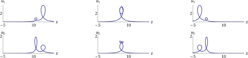
Figure 1: Parametric plots (with parameter $\bar{x}$) of the two components $u_{1}$ and $u_{2}$ for a 2-soliton solution of the 2-component short pulse equation (5.11) with $\epsilon=-1$, determined by the data of Example 5.3 with $N=2$, $s_{1}=1$, $s_{2}=2$ and $C=\mathrm{diag}(1+3\mathrm{i},1-3\mathrm{i},2+\mathrm{i}/2,2-\mathrm{i}/2)$ at $x=-3,-1,1$.

Remark 5.4.

In order to obtain a Lax pair for the short pulse equation, we start with

$$\psi_{x}=\left(L-\frac{\nu}{2}I\right)\psi,\qquad\psi_{\bar{x}}=\left(\bar{L}-\frac{1}{2\nu}I\right)\psi,$$

with $L$ and $\bar{L}$ taken from Remarks 3.2 and 4.2, respectively. Without imposing a reduction, the integrability conditions are (5.4) and (5.5) (modulo an integration with respect to $\bar{x}$). Writing $\psi(x,\bar{x})=\chi(x,z(x,\bar{x}))$, we find

$$\chi_{z}=(\bar{L}-\frac{1}{2\nu}I)\chi=\frac{1}{2\nu}\left(\begin{array}[]{cc}I&-u_{z}\\ \epsilon u_{z}&-I\end{array}\right)\chi,$$

$$\chi_{x}=(L-\frac{\nu}{2}I)\chi-z_{x}\chi_{z}=\frac{1}{2}\left(\begin{array}[]{cc}\nu&u\\ \epsilon u&-\nu\end{array}\right)\chi-\frac{\epsilon}{2}u^{2}\chi_{z}$$

$$\phantom{\chi_{x}}{}=\left(\begin{array}[]{cc}\frac{\nu}{2}I-\frac{\epsilon}{4\nu}u^{2}&\frac{1}{2}u+\frac{\epsilon}{4\nu}u^{2}u_{z}\vspace{1mm}\\ \frac{\epsilon}{2}u-\frac{1}{4\nu}u^{2}u_{z}&-\frac{\nu}{2}I+\frac{\epsilon}{4\nu}u^{2}\end{array}\right)\chi,$$

where we applied the reduction conditions (5.6) and used (5.7), (5.8) and (5.9). Using the symmetry $u\mapsto-u$ of the short pulse equation, we recover the Lax pair given in [37] for the scalar case and with $\epsilon=-1$.

6 Dual AKNS hierarchies

For the bidifferential calculus determined by (3.13), the Miura transformation (2.3) with $\Delta=0$ takes the form

$$\lambda^{-1}\big{(}g-g_{-[\lambda]}\big{)}g^{-1}=\mathcal{P}\phi-\phi_{-[\lambda]}\mathcal{P},$$ (6.1)

and the dual equation (2.4) becomes

$$\mu^{-1}\left(\mathcal{P}g_{-[\mu]}g^{-1}-(g_{-[\mu]}g^{-1})_{-[\lambda]}\mathcal{P}\right)=\lambda^{-1}\left(\mathcal{P}g_{-[\lambda]}g^{-1}-(g_{-[\lambda]}g^{-1})_{-[\mu]}\mathcal{P}\right).$$

Multiplying from the left by $g^{-1}_{-[\lambda]-[\mu]}$ and from the right by $g$, this can be written as

$$\mu^{-1}\left(g^{-1}_{-[\lambda]}\mathcal{P}g-(g^{-1}_{-[\lambda]}\mathcal{P}g)_{-[\mu]}\right)=\lambda^{-1}\left(g^{-1}_{-[\mu]}\mathcal{P}g-(g^{-1}_{-[\mu]}\mathcal{P}g)_{-[\lambda]}\right).$$ (6.2)

To order $\mu^{0}$ this yields

$$\lambda^{-1}\left(g^{-1}\mathcal{P}g-(g^{-1}\mathcal{P}g)_{-[\lambda]}\right)=(g^{-1}_{-[\lambda]}\mathcal{P}g)_{x}.$$ (6.3)

Applying a Miwa shift with $-[\mu]$ and subtracting the result from this equation, we obtain

$$\mu^{-1}\left(g^{-1}_{-[\lambda]}\mathcal{P}g-(g^{-1}_{-[\lambda]}\mathcal{P}g)_{-[\mu]}\right)_{x}$$

$$\qquad=\lambda^{-1}\mu^{-1}\Big{(}g^{-1}\mathcal{P}g-(g^{-1}\mathcal{P}g)_{-[\lambda]}-(g^{-1}\mathcal{P}g)_{-[\mu]}+(g^{-1}\mathcal{P}g)_{-[\lambda]-[\mu]}\Big{)}.$$

Since the r.h.s. is symmetric in $\lambda$, $\mu$, this implies (6.2) up to an $x$-independent “constant of integration”. Hence (6.2) reduces to (6.3). The first non-trivial equation resulting from an expansion of (6.3) in powers of the indeterminate $\lambda$ is obtained as the term linear in $\lambda$,

$$(g^{-1}\mathcal{P}g)_{t_{2}}-(g^{-1}\mathcal{P}g)_{xx}=-2\left((g^{-1})_{x}\mathcal{P}g\right)_{x}.$$ (6.4)

6.1 Miura transformation and relation
with the generalized Heisenberg magnet model

Introducing

$$\mathcal{S}=g^{-1}Jg$$

(see also [19]), we have the identities

$$\mathcal{S}_{t_{n}}=[\mathcal{S},g^{-1}g_{t_{n}}],\qquad n=1,2,\ldots,$$ (6.5)

and

$$\mathcal{S}^{2}=I\quad\Rightarrow\quad\mathcal{S}_{x}\mathcal{S}=-\mathcal{S}\mathcal{S}_{x}\quad\Rightarrow\quad\mathcal{S}_{x}{}^{2}=-\frac{1}{2}\{\mathcal{S},\mathcal{S}_{xx}\}\quad\Rightarrow\quad(\mathcal{S}\mathcal{S}_{x})_{x}=\frac{1}{2}[\mathcal{S},\mathcal{S}_{xx}].$$ (6.6)

The dual hierarchy equation (6.4) can now be expressed as follows,

$$\mathcal{S}_{t_{2}}=\mathcal{S}_{xx}+2\left(g^{-1}g_{x}(I+\mathcal{S})\right)_{x}.$$

In order to express this solely in terms of $\mathcal{S}$ we use the Miura transformation (6.1), which to order $\lambda^{0}$ reads

$$g_{x}g^{-1}=[\mathcal{P},\phi]=\frac{1}{2}[J,\phi].$$ (6.7)

This imposes the following condition on $g$,

$$\big{\{}J,g_{x}g^{-1}\big{\}}=0,$$ (6.8)

which can be expressed as $\{\mathcal{S},g^{-1}g_{x}\}=0$, hence together with (6.5) we have

$$g^{-1}g_{x}=-\frac{1}{2}\mathcal{S}_{x}\mathcal{S}=:\mathcal{F}^{(1)}.$$ (6.9)

Inserting this in the expression for $\mathcal{S}_{t_{2}}$, and using the above identities, leads to

$$\mathcal{S}_{t_{2}}=\mathcal{S}_{xx}-\left(\mathcal{S}_{x}\mathcal{S}(I+\mathcal{S})\right)_{x}=\frac{1}{2}[\mathcal{S},\mathcal{S}_{xx}]=2\mathcal{F}^{(1)}_{x},$$ (6.10)

which is the (generalized) Heisenberg magnet equation (see also Remark 4.1).

Remark 6.1.

The ordinary Heisenberg magnet equation $\vec{S}_{t}=\vec{S}\times\vec{S}_{xx}$ is obtained from the $2\times 2$ matrix case by writing $\mathcal{S}=\sum_{k=1}^{3}S_{k}\sigma_{k}$, where $\sigma_{1},\sigma_{2},\sigma_{3}$ are the Pauli matrices, and setting $t_{2}=-\mathrm{i}t$.

More generally, with the help of the Miura transformation (6.1) the hierarchy equations resulting from (6.3) can be expressed solely in terms of $\mathcal{S}$. (6.1) implies

$$\lambda^{-1}\big{\{}J,(g-g_{-[\lambda]})g^{-1}\big{\}}=\{J,\mathcal{P}\phi-\phi_{-[\lambda]}\mathcal{P}\}=\left(\begin{array}[]{cc}2(p-p_{-[\lambda]})&0\\ 0&0\end{array}\right)=\left(\begin{array}[]{cc}-2\lambda q\bar{q}_{-[\lambda]}&0\\ 0&0\end{array}\right)$$

$$\phantom{\lambda^{-1}\big{\{}J,(g-g_{-[\lambda]})g^{-1}\big{\}}}{}=-2\lambda\mathcal{P}[\mathcal{P},\phi][\mathcal{P},\phi]_{-[\lambda]}\mathcal{P}=-2\lambda\mathcal{P}g_{x}g^{-1}(g_{x}g^{-1})_{-[\lambda]}\mathcal{P},$$

where we assumed that (3.20) holds and used (6.7) in the last step. Multiplication from the left by $g^{-1}$ and from the right by $g$ leads to

$$\lambda^{-1}\big{\{}\mathcal{S},g^{-1}(g-g_{-[\lambda]})\big{\}}=-\frac{1}{4}\lambda(I+\mathcal{S})\mathcal{S}_{x}g^{-1}g_{x,-[\lambda]}g^{-1}_{-[\lambda]}g(I+\mathcal{S}),$$ (6.11)

where we used $g^{-1}\mathcal{P}g=\frac{1}{2}(I+\mathcal{S})$, (6.9), and $\mathcal{S}^{2}=I$. At order $\lambda^{1}$ we obtain

$$\big{\{}\mathcal{S},g^{-1}(g_{t_{2}}-g_{xx})\big{\}}=-\frac{1}{2}(I+\mathcal{S})\mathcal{S}_{x}g^{-1}g_{x}(I+\mathcal{S})=\frac{1}{4}(I+\mathcal{S})\mathcal{S}_{x}{}^{2}(I+\mathcal{S})=\frac{1}{2}\mathcal{S}_{x}{}^{2}(I+\mathcal{S}),$$

hence, using (6.6) and (6.9),

$$\big{\{}\mathcal{S},g^{-1}g_{t_{2}}\big{\}}=\big{\{}\mathcal{S},g^{-1}g_{xx}\big{\}}+\frac{1}{2}\mathcal{S}_{x}{}^{2}(I+\mathcal{S})$$

$$\phantom{\big{\{}\mathcal{S},g^{-1}g_{t_{2}}\big{\}}}{}=\left\{\mathcal{S},-\frac{1}{2}(\mathcal{S}_{x}\mathcal{S})_{x}+\frac{1}{4}(\mathcal{S}_{x}\mathcal{S})^{2}\right\}+\frac{1}{2}\mathcal{S}_{x}{}^{2}(I+\mathcal{S})=\frac{1}{2}\mathcal{S}_{x}{}^{2}.$$ (6.12)

With the help of (6.10), (6.5) together with (6.12) implies

$$g^{-1}g_{t_{2}}=\frac{1}{2}\mathcal{S}_{xx}+\frac{3}{4}\mathcal{S}_{x}{}^{2}\mathcal{S}=:\mathcal{F}_{2}.$$ (6.13)

At order $\lambda^{2}$, (6.3) yields

$$\mathcal{S}_{t_{3}}=\left(\frac{3}{2}\mathcal{S}_{t_{2}}-\frac{1}{2}\mathcal{S}_{xx}+\frac{3}{2}\big{(}g^{-1}g_{t_{2}}+\big{(}g^{-1}\big{)}_{xx}g\big{)}(I+\mathcal{S})\right)_{x}.$$

With the help of (6.9) and (6.13), this can be arranged into the form

$$\mathcal{S}_{t_{3}}=\left(-\frac{3}{2}\mathcal{S}_{xx}\mathcal{S}-\frac{3}{2}\mathcal{S}_{x}{}^{2}-\frac{1}{2}\mathcal{S}_{xx}+\frac{3}{2}\mathcal{S}_{xx}(I+\mathcal{S})+\frac{3}{2}\mathcal{S}_{x}{}^{2}(I+\mathcal{S})\right)_{x}$$

$$\phantom{\mathcal{S}_{t_{3}}}{}=\left(\mathcal{S}_{xx}+\frac{3}{2}\mathcal{S}_{x}{}^{2}\mathcal{S}\right)_{x}=2\mathcal{F}^{(2)}_{x}.$$

In a similar way, from (6.3) and (6.11) we obtain

$$g^{-1}g_{t_{3}}=-\frac{1}{2}(\mathcal{S}_{xx}\mathcal{S})_{x}-\mathcal{S}_{x}\mathcal{S}_{xx}-\frac{5}{4}\mathcal{S}_{x}{}^{3}\mathcal{S}=:\mathcal{F}^{(3)},$$

$$g^{-1}g_{t_{4}}=\frac{15}{8}\mathcal{S}_{x}{}^{2}\mathcal{S}_{xx}+\frac{5}{4}\mathcal{S}_{x}\mathcal{S}_{xx}\mathcal{S}_{x}+\frac{5}{4}\mathcal{S}_{x}\mathcal{S}_{xxx}\mathcal{S}+\frac{5}{8}\mathcal{S}_{xx}\mathcal{S}_{x}{}^{2}+\frac{5}{4}\mathcal{S}_{xx}{}^{2}\mathcal{S}$$

$$\phantom{g^{-1}g_{t_{4}}=}{}+\frac{5}{4}\mathcal{S}_{xxx}\mathcal{S}_{x}\mathcal{S}+\frac{35}{16}\mathcal{S}_{x}{}^{4}\mathcal{S}+\frac{1}{2}\mathcal{S}_{xxxx}=:\mathcal{F}^{(4)},$$

and

$$\mathcal{S}_{t_{n}}=2\mathcal{F}^{(n-1)}_{x},\qquad n=2,3,4,5,$$

which likely extends to all higher $n\in\mathbb{N}$. Of course, the expression for $\mathcal{S}_{t_{n}}$ can be recovered by inserting the corresponding expression for $g^{-1}g_{t_{n}}$ in (6.5).

Remark 6.2.

Conditions like (6.8) originated from the use of the Miura transformation, and they are in fact needed to express the original hierarchy for the matrix variable $g$ in terms of $\mathcal{S}$. The “mismatch” in the Miura transformation, leading to the restriction of the form of $g$, can be traced back to the fact that in the step from (2.4) to (2.3) we are dropping cohomological terms (see Remark 3.7).

Example 6.3.

If $m=2$, we write

$$g^{-1}=\left(\begin{array}[]{cc}\kappa&-\sigma\\ -\bar{\sigma}&\bar{\kappa}\end{array}\right),\qquad\mbox{hence}\qquad g=\frac{1}{\kappa\bar{\kappa}-\sigma\bar{\sigma}}\left(\begin{array}[]{cc}\bar{\kappa}&\sigma\\ \bar{\sigma}&\kappa\end{array}\right),$$

and thus

$$\mathcal{S}=g^{-1}Jg=\frac{1}{\kappa\bar{\kappa}-\sigma\bar{\sigma}}\left(\begin{array}[]{cc}\kappa\bar{\kappa}+\sigma\bar{\sigma}&2\kappa\sigma\\ -2\bar{\kappa}\bar{\sigma}&-\kappa\bar{\kappa}-\sigma\bar{\sigma}\end{array}\right).$$

The condition (6.8) amounts to $\kappa_{x}\bar{\kappa}-\sigma_{x}\bar{\sigma}=0$ and $\kappa\bar{\kappa}_{x}-\sigma\bar{\sigma}_{x}=0$. By adding these two equations, we find that

$$(\kappa\bar{\kappa}-\sigma\bar{\sigma})_{x}=0.$$ (6.14)

Remark 6.4.

Using the Miura transformation (2.3), the linear equation (3.27) reads

$$\bar{\mathrm{d}}\Psi=\big{[}(\bar{\mathrm{d}}g)g^{-1}\big{]}\Psi+2z\mathrm{d}\Psi$$

(writing $\nu=2z$), hence

$$\bar{\mathrm{d}}\hat{\psi}=2z\big{[}\mathrm{d}\hat{\psi}+g^{-1}(\mathrm{d}g)\hat{\psi}\big{]}$$

in terms of

$$\hat{\psi}=g^{-1}\Psi.$$

Evaluation of the linear equation for the bidifferential calculus given by (3.13) leads to

$$\lambda^{-1}\hat{\psi}-\lambda^{-1}\hat{\psi}_{-[\lambda]}(I-2z\lambda\mathcal{P})=2z\big{(}g^{-1}_{-[\lambda]}\mathcal{P}g\big{)}\hat{\psi}.$$

Writing

$$\hat{\psi}=\psi e^{-\sum_{n\geq 1}(2z\mathcal{P})^{n}t_{n}},$$

we obtain

$$\lambda^{-1}(\psi-\psi_{-[\lambda]})=2z\big{(}g^{-1}_{-[\lambda]}\mathcal{P}g\big{)}\psi=z\big{(}g^{-1}_{-[\lambda]}g\big{)}(I+\mathcal{S})\psi.$$

Expansion in powers of $\lambda$ yields

$$\psi_{x}=z(I+\mathcal{S})\psi,$$

$$\psi_{t_{2}}=\big{[}2z^{2}(I+\mathcal{S})-z\mathcal{S}_{x}\mathcal{S}\big{]}\psi,$$

$$\psi_{t_{3}}=\left[4z^{3}(I+\mathcal{S})-2z^{2}\mathcal{S}_{x}\mathcal{S}+\frac{z}{2}\big{(}2\mathcal{S}_{xx}+3\mathcal{S}_{x}{}^{2}\mathcal{S}\big{)}\right]\psi,$$

$$\psi_{t_{4}}=\Bigg{[}8z^{4}(I+\mathcal{S})-4z^{3}\mathcal{S}_{x}\mathcal{S}+z^{2}\big{(}2\mathcal{S}_{xx}+3\mathcal{S}_{x}{}^{2}\mathcal{S}\big{)}$$

$$\hphantom{\psi_{t_{4}}=}{}-\frac{z}{2}\big{(}2\mathcal{S}_{xxx}\mathcal{S}-2\mathcal{S}_{xx}\mathcal{S}_{x}-4\mathcal{S}_{x}\mathcal{S}_{xx}-5\mathcal{S}_{x}{}^{3}\mathcal{S}\big{)}\Bigg{]}\psi.$$

The first two equations constitute a Lax pair for the generalized Heisenberg magnet equation (with $\mathcal{S}^{2}=I$).

6.2 A class of solutions

The following result is an analog to that in Section 3.3 (see also Remark 3 in [2]). It allows to generate solutions of (2.4) from solutions of a linear system.

Theorem 6.5.

Let $(\Omega,\mathrm{d},\bar{\mathrm{d}})$ be a bidifferential calculus with $\Omega=\mathcal{A}\otimes\bigwedge(\mathbb{C}^{N})$ and $\mathcal{A}=\mathrm{Mat}_{n_{0}}(\mathcal{B})$, for some $n_{0}\in\mathbb{N}$. For fixed $n\geq n_{0}$, let $\boldsymbol{S}\in\mathrm{Mat}(n,n,\mathcal{B})$ and $\Delta\in\mathrm{Mat}(m,m,\mathcal{B})$. Furthermore, let $\boldsymbol{X}\in\mathrm{Mat}(n,n,\mathcal{B})$ and $\boldsymbol{W}\in\mathrm{Mat}(m,n,\mathcal{B})$ satisfy the linear equations

$$\bar{\mathrm{d}}\boldsymbol{X}=(\mathrm{d}\boldsymbol{X})\boldsymbol{S},\qquad\bar{\mathrm{d}}\boldsymbol{W}=(\mathrm{d}\boldsymbol{W})\boldsymbol{S},$$

and also

$$\boldsymbol{X}\boldsymbol{S}-\boldsymbol{R}\boldsymbol{X}=\tilde{\boldsymbol{V}}\boldsymbol{Z},\qquad\boldsymbol{W}\boldsymbol{S}-\Delta\boldsymbol{W}=\boldsymbol{C}\boldsymbol{X},$$ (6.15)

with matrices $\boldsymbol{C},\boldsymbol{Z}\in\mathrm{Mat}(m,n,\mathcal{B})$, $\boldsymbol{R}\in\mathrm{Mat}(n,n,\mathcal{B})$ and $\tilde{\boldsymbol{V}}\in\mathrm{Mat}(n,m,\mathcal{B})$, satisfying

$$\mathrm{d}\boldsymbol{C}=0,\qquad\mathrm{d}\boldsymbol{R}=0,\qquad\mathrm{d}\tilde{\boldsymbol{V}}=0,\qquad\bar{\mathrm{d}}\tilde{\boldsymbol{V}}=0.$$

Then

$$g=\big{(}\boldsymbol{W}\boldsymbol{X}^{-1}\tilde{\boldsymbol{V}}\big{)}^{-1},$$ (6.16)

provided the inverse exists, solves the $($modified$)$ Miura transformation equation (2.3), i.e.

$$[\bar{\mathrm{d}}g-(\mathrm{d}g)\Delta]g^{-1}=\mathrm{d}\phi,$$ (6.17)

with some $m\times m$ matrix $\phi$, and thus $($by application of $\mathrm{d})$ also (2.4), i.e.

$$\mathrm{d}\big{(}\left(\bar{\mathrm{d}}g-(\mathrm{d}g)\Delta\right)g^{-1}\big{)}=0.$$ (6.18)

Proof 6.6.

Using the Leibniz rule and the assumptions, we have

$$\bar{\mathrm{d}}g^{-1}=(\bar{\mathrm{d}}\boldsymbol{W})\boldsymbol{X}^{-1}\tilde{\boldsymbol{V}}-\boldsymbol{W}\boldsymbol{X}^{-1}(\bar{\mathrm{d}}\boldsymbol{X})\boldsymbol{X}^{-1}\tilde{\boldsymbol{V}}$$

$$\phantom{\bar{\mathrm{d}}g^{-1}}{}=(\mathrm{d}\boldsymbol{W})\boldsymbol{S}\boldsymbol{X}^{-1}\tilde{\boldsymbol{V}}-\boldsymbol{W}\boldsymbol{X}^{-1}(\mathrm{d}\boldsymbol{X})\boldsymbol{S}\boldsymbol{X}^{-1}\tilde{\boldsymbol{V}}=\big{(}\mathrm{d}\boldsymbol{W}-\boldsymbol{W}\boldsymbol{X}^{-1}\mathrm{d}\boldsymbol{X}\big{)}\boldsymbol{S}\boldsymbol{X}^{-1}\tilde{\boldsymbol{V}}$$

$$\phantom{\bar{\mathrm{d}}g^{-1}}{}=\mathrm{d}\big{(}\boldsymbol{W}\boldsymbol{X}^{-1}\big{)}\boldsymbol{X}\boldsymbol{S}\boldsymbol{X}^{-1}\tilde{\boldsymbol{V}}=\mathrm{d}\big{(}\boldsymbol{W}\boldsymbol{S}\boldsymbol{X}^{-1}\tilde{\boldsymbol{V}}\big{)}-\boldsymbol{W}\boldsymbol{X}^{-1}\mathrm{d}\big{(}\boldsymbol{X}\boldsymbol{S}\boldsymbol{X}^{-1}\tilde{\boldsymbol{V}}\big{)}$$

$$\phantom{\bar{\mathrm{d}}g^{-1}}{}=\mathrm{d}\big{(}\Delta g^{-1}\big{)}-\boldsymbol{W}\boldsymbol{X}^{-1}\mathrm{d}\big{[}(\boldsymbol{R}\boldsymbol{X}+\tilde{\boldsymbol{V}}\boldsymbol{Z})\boldsymbol{X}^{-1}\tilde{\boldsymbol{V}}\big{]}=\mathrm{d}\big{(}\Delta g^{-1}\big{)}-g^{-1}\mathrm{d}\big{(}\boldsymbol{Z}\boldsymbol{X}^{-1}\tilde{\boldsymbol{V}}\big{)},$$

and thus

$$[\bar{\mathrm{d}}g-(\mathrm{d}g)\Delta]g^{-1}=\mathrm{d}\big{(}\boldsymbol{Z}\boldsymbol{X}^{-1}\tilde{\boldsymbol{V}}-g\Delta g^{-1}\big{)}.$$ ∎

Remark 6.7.

The assumptions in Theorem 6.5 give rise to integrability conditions. The latter are satisfied if

$$\bar{\mathrm{d}}\boldsymbol{S}=(\mathrm{d}\boldsymbol{S})\boldsymbol{S},\qquad\bar{\mathrm{d}}\Delta=(\mathrm{d}\Delta)\Delta,\qquad\bar{\mathrm{d}}\boldsymbol{C}=(\mathrm{d}\Delta)\boldsymbol{C},\qquad\bar{\mathrm{d}}\boldsymbol{Z}=(\mathrm{d}\boldsymbol{Z})\boldsymbol{S}.$$

In the following we exploit Theorem 6.5 for the bidifferential calculus given by (3.13) with some simplifications. We set $\Delta=0$ and make the further assumption that $\boldsymbol{S}$ is $\mathrm{d}$- and $\bar{\mathrm{d}}$-constant, and we write $\boldsymbol{Z}=\tilde{\boldsymbol{U}}\boldsymbol{Y}$, where $\tilde{\boldsymbol{U}}\in\mathrm{Mat}(m,n,\mathcal{B})$ is $\mathrm{d}$- and $\bar{\mathrm{d}}$-constant and $\boldsymbol{Y}\in\mathrm{Mat}(n,n,\mathcal{B})$ solves $\bar{\mathrm{d}}\boldsymbol{Y}=(\mathrm{d}\boldsymbol{Y})\boldsymbol{S}$. This is motivated by the fact that then the first of conditions (6.15) reduces to (3.31), i.e.

$$\boldsymbol{S}\boldsymbol{K}-\boldsymbol{K}\boldsymbol{S}=\boldsymbol{V}\boldsymbol{U},$$ (6.19)

assuming that $\boldsymbol{A}_{d}$ is invertible and using results from Section 3.3, in particular the definitions (3.32) for $\boldsymbol{K}$, $\boldsymbol{U}$, $\boldsymbol{V}$. Furthermore, we obtain

$$\boldsymbol{W}=\boldsymbol{W}_{d}+\boldsymbol{W}_{o}\boldsymbol{\Xi},\qquad\boldsymbol{\Xi}=e^{-\xi(\boldsymbol{S})\boldsymbol{J}},\qquad\xi(\boldsymbol{S})=\sum_{k\geq 1}\boldsymbol{S}^{k}t_{k},$$

and the second of conditions (6.15) yields $\boldsymbol{C}=\boldsymbol{W}_{d}\boldsymbol{S}\boldsymbol{A}_{d}^{-1}$ (which simply determines $\boldsymbol{C}$) and, assuming that $\boldsymbol{S}$ is invertible,

$$\boldsymbol{W}_{o}=-\boldsymbol{W}_{d}\boldsymbol{S}\boldsymbol{K}\boldsymbol{S}^{-1}.$$

The solution (6.16) of (6.18) (with $\Delta=0$) is then given by

$$g^{-1}=\boldsymbol{W}_{d}\big{(}\boldsymbol{I}-\boldsymbol{S}\boldsymbol{K}\boldsymbol{S}^{-1}\boldsymbol{\Xi}\big{)}(\boldsymbol{I}-\boldsymbol{K}\boldsymbol{\Xi})^{-1}\boldsymbol{V}.$$

Rewriting this as

$$g^{-1}=\boldsymbol{W}_{d}\big{(}\boldsymbol{I}-\boldsymbol{S}\boldsymbol{K}\boldsymbol{S}^{-1}\boldsymbol{\Xi}\big{)}(I+\boldsymbol{K}\boldsymbol{\Xi})\big{(}\boldsymbol{I}-(\boldsymbol{K}\boldsymbol{\Xi})^{2}\big{)}^{-1}\boldsymbol{V}$$

$$\phantom{g^{-1}}{}=\boldsymbol{W}_{d}\big{(}\boldsymbol{I}-\boldsymbol{S}\boldsymbol{K}\boldsymbol{S}^{-1}\boldsymbol{\Xi}-\boldsymbol{S}\boldsymbol{K}\boldsymbol{S}^{-1}\boldsymbol{\Xi}\boldsymbol{K}\boldsymbol{\Xi}+\boldsymbol{K}\boldsymbol{\Xi}\big{)}\big{(}\boldsymbol{I}-(\boldsymbol{K}\boldsymbol{\Xi})^{2}\big{)}^{-1}\boldsymbol{V},$$

it can easily be decomposed into a part that commutes with $J$,

$$\big{(}g^{-1}\big{)}_{d}=\boldsymbol{W}_{d}\big{(}\boldsymbol{I}-\boldsymbol{S}\boldsymbol{K}\boldsymbol{S}^{-1}\boldsymbol{\Xi}\boldsymbol{K}\boldsymbol{\Xi}\big{)}\big{(}\boldsymbol{I}-(\boldsymbol{K}\boldsymbol{\Xi})^{2}\big{)}^{-1}\boldsymbol{V}$$

$$\phantom{\big{(}g^{-1}\big{)}_{d}}{}=\boldsymbol{W}_{d}\boldsymbol{V}+\boldsymbol{W}_{d}(\boldsymbol{K}\boldsymbol{S}-\boldsymbol{S}\boldsymbol{K})\boldsymbol{S}^{-1}\boldsymbol{\Xi}\boldsymbol{K}\boldsymbol{\Xi}\big{(}\boldsymbol{I}-(\boldsymbol{K}\boldsymbol{\Xi})^{2}\big{)}^{-1}\boldsymbol{V}$$

$$\phantom{\big{(}g^{-1}\big{)}_{d}}{}=\boldsymbol{W}_{d}\boldsymbol{V}\big{[}\boldsymbol{I}-\boldsymbol{U}\boldsymbol{S}^{-1}\boldsymbol{\Xi}\boldsymbol{K}\boldsymbol{\Xi}\big{(}\boldsymbol{I}-(\boldsymbol{K}\boldsymbol{\Xi})^{2}\big{)}^{-1}\boldsymbol{V}\big{]},$$

and a part that anti-commutes with $J$,

$$\big{(}g^{-1}\big{)}_{o}=\boldsymbol{W}_{d}(\boldsymbol{K}\boldsymbol{S}-\boldsymbol{S}\boldsymbol{K})\boldsymbol{S}^{-1}\boldsymbol{\Xi}\big{(}\boldsymbol{I}-(\boldsymbol{K}\boldsymbol{\Xi})^{2}\big{)}^{-1}\boldsymbol{V}$$

$$\phantom{\big{(}g^{-1}\big{)}_{o}}{}=-\boldsymbol{W}_{d}\boldsymbol{V}\boldsymbol{U}\boldsymbol{S}^{-1}\boldsymbol{\Xi}\big{(}\boldsymbol{I}-(\boldsymbol{K}\boldsymbol{\Xi})^{2}\big{)}^{-1}\boldsymbol{V}.$$

Using our concrete form of $J$ and $\boldsymbol{J}$, the matrices $\boldsymbol{K}$, $\boldsymbol{S}$, $\boldsymbol{U}$, $\boldsymbol{V}$ have the form given in (3.46), and we have

$$\boldsymbol{W}_{d}=\left(\begin{array}[]{cc}W&0\\ 0&\bar{W}\end{array}\right),\qquad\boldsymbol{\Xi}=\left(\begin{array}[]{cc}\Xi&0\\ 0&\bar{\Xi}\end{array}\right),\qquad\Xi=e^{-\xi(S)},\qquad\bar{\Xi}=e^{\xi(-\bar{S})}.$$

This leads to

$$g^{-1}=\left(\begin{array}[]{cc}\kappa&-\sigma\\ -\bar{\sigma}&\bar{\kappa}\end{array}\right)$$

where

$$\kappa=(WV)\big{[}I+U\bar{S}^{-1}\bar{\Xi}\bar{K}\Xi(I-K\bar{\Xi}\bar{K}\Xi)^{-1}V\big{]},$$

$$\bar{\kappa}=(\bar{W}\bar{V})\big{[}I+\bar{U}S^{-1}\Xi K\bar{\Xi}(I-\bar{K}\Xi K\bar{\Xi})^{-1}\bar{V}\big{]},$$

$$\sigma=-(WV)U\bar{S}^{-1}\bar{\Xi}(I-\bar{K}\Xi K\bar{\Xi})^{-1}\bar{V},$$

$$\bar{\sigma}=-(\bar{W}\bar{V})\bar{U}S^{-1}\Xi(I-K\bar{\Xi}\bar{K}\Xi)^{-1}V.$$

The only restrictions that have to be imposed on the matrices $K$, $\bar{K}$, $S$, $\bar{S}$, $U$, $\bar{U}$, $V$, $\bar{V}$ result from (6.19). They are

$$SK+K\bar{S}=VU,\qquad\bar{S}\bar{K}+\bar{K}S=\bar{V}\bar{U}.$$ (6.20)

The solutions of the hierarchy for $g$ obtained in this way also determine solutions of the generalized Heisenberg hierarchy. This is so because the solutions constructed above via Theorem 6.5 are actually solutions of the Miura transformation and our choice of matrix data via Proposition 3.4 ensures that (3.20) holds (which we used in Section 6.1).

6.3 Reciprocal dual and combined dual AKNS hierarchies

Elaborating the dual equation (2.4) with the “reciprocal” bidifferential calculus determined by (4.1), instead of using that determined by (3.13), we simply obtain (6.2) with $g$ replaced by $g^{-1}$. Again, we can combine the dual AKNS hierarchy and its reciprocal version, adopting the procedure in Section 5. New equations arise from the mixed parts, hence from evaluating (2.4) using the bidifferential calculus given by

$$\mathrm{d}f=[\mathcal{P}\mathbb{E}_{\lambda},f]\zeta+\mu^{-1}[\bar{\mathbb{E}}_{\mu},f]\bar{\zeta},\qquad\bar{\mathrm{d}}f=\lambda^{-1}[\mathbb{E}_{\lambda},f]\zeta+[\mathcal{P}\bar{\mathbb{E}}_{\mu},f]\bar{\zeta},$$

which is a constituent of the calculus determined by (5.1). This results in

$$\big{[}\mathcal{P}g_{-\bar{[\mu]}}\mathcal{P}g^{-1}-\big{(}g_{-\bar{[\mu]}}\mathcal{P}g^{-1}\big{)}_{-[\lambda]}\mathcal{P}\big{]}-\mu^{-1}\lambda^{-1}\big{[}g_{-[\lambda]}g^{-1}-\big{(}g_{-[\lambda]}g^{-1}\big{)}_{-\bar{[\mu]}}\big{]}=0.$$

To order $\lambda^{0}\mu^{0}$ this is

$$\big{(}g_{x}g^{-1}\big{)}_{\bar{x}}+\big{[}\mathcal{P},g\mathcal{P}g^{-1}\big{]}=0,$$

hence

$$\big{(}g_{x}g^{-1}\big{)}_{\bar{x}}=\frac{1}{4}\big{(}g\tilde{g}^{-1}-\tilde{g}g^{-1}\big{)}\qquad\mbox{where}\qquad\tilde{g}=JgJ.$$ (6.21)

The Miura transformation between the combined hierarchies consists of a pair of Miura transformations, one for the original hierarchy and another one for the reciprocal. It results in the following two generating equations,

$$\lambda^{-1}\big{(}g-g_{-[\lambda]}\big{)}g^{-1}=\mathcal{P}\phi-\phi_{-[\lambda]}\mathcal{P},\qquad\big{(}\mathcal{P}g-g_{-\bar{[\lambda]}}\mathcal{P}\big{)}g^{-1}=\lambda^{-1}\big{(}\phi-\phi_{-\bar{[\lambda]}}\big{)}.$$

In particular, this yields

$$g_{x}g^{-1}=[\mathcal{P},\phi],\qquad\phi_{\bar{x}}=[\mathcal{P},g]g^{-1}.$$ (6.22)

The formulas in Section 6.2 still generate solutions of the combined dual hierarchy and also of the Miura transformation (cf. (6.17)), provided we extend the expression for $\xi(S)$ used there to

$$\xi(S)=\sum_{k\geq 1}S^{k}t_{k}+\sum_{k\geq 1}S^{-k}\bar{t}_{k}.$$ (6.23)

6.3.1 Sine-Gordon solutions

If $m=2$ and if $g$ has the form

$$g=f\left(\begin{array}[]{cc}\cos(\vartheta/2)&-\sin(\vartheta/2)\\ \sin(\vartheta/2)&\cos(\vartheta/2)\end{array}\right)=fe^{\mathbb{I}\vartheta/2},\qquad\mathbb{I}=\left(\begin{array}[]{cc}0&-1\\ 1&0\end{array}\right),$$

where $f$ is a function independent of $x$, then (6.21) becomes the sine-Gordon equation

$$\vartheta_{x\bar{x}}=\sin(\vartheta).$$

The function $f$ drops out of equation (6.21). As a consequence of the form of $g$, the condition (6.8), which arose from the Miura transformation, is satisfied. (6.22) requires the reduction conditions (5.6) with $\epsilon=-1$ and then reads

$$q=-\frac{1}{2}\vartheta_{x},\qquad q_{\bar{x}}=-\frac{1}{2}\sin(\vartheta),\qquad p_{\bar{x}}=\frac{1}{2}[1-\cos(\vartheta)].$$

In order to generate solutions of the sine-Gordon equation (and more generally of the corresponding hierarchy), we have to choose the matrix data in such a way that $g$ has the above form. We set

$$\bar{K}=-K,\qquad\bar{S}=S,\qquad\bar{U}=-U,\qquad\bar{V}=V,\qquad\bar{W}=W.$$

Then (6.20) reduces to a single Sylvester equation, $SK+KS=VU$. Setting $t_{2k}=\bar{t}_{2k}=0$, $k=1,2,\ldots$, (6.23) has the property $\xi(-S)=-\xi(S)$. As a consequence, we have $\bar{\Xi}=e^{\xi(-S)}=e^{-\xi(S)}=\Xi$ and thus

$$\kappa=\bar{\kappa}=\alpha\big{[}I-US^{-1}\Xi K\Xi\big{(}I+(K\Xi)^{2}\big{)}^{-1}V\big{]},\qquad\sigma=-\bar{\sigma}=-\alpha US^{-1}\Xi\big{(}I+(K\Xi)^{2}\big{)}^{-1}V,$$

where $\alpha=WV$. We still have to ensure that $\kappa^{2}+\sigma^{2}=f^{2}$, with some function $f$ that does not depend on $x$. But since our procedure actually solves the Miura transformation (recall (6.17)), we already know that (6.8) is satisfied, hence (6.14) holds, which shows that $\kappa^{2}+\sigma^{2}$ indeed does not depend on $x$.

Example 6.8.

Let $n=1$, $S=s\in\mathbb{R}$, and $U=V=W=1$. Then the Sylvester equation $SK+KS=VU$ is solved by $K=\frac{1}{2s}$. Writing $\Xi=2se^{-\tilde{\xi}(s)}$, where $\tilde{\xi}(s)=\sum_{k\geq 0}(s^{2k+1}t_{2k+1}+s^{-2k-1}\bar{t}_{2k+1})+\xi_{0}$ with a constant $\xi_{0}$, we obtain $\kappa=\tanh\tilde{\xi}(s)$ and $\sigma=\mathrm{sech}\tilde{\xi}(s)$, so that $\kappa^{2}{+}\sigma^{2}{=}1$. From $\sigma/\kappa=\mathrm{csch}\tilde{\xi}(s)$ then follows the well-known kink solution $\vartheta=2\arctan(\mathrm{csch}\tilde{\xi}(s))=4\arctan e^{\tilde{\xi}(s)}$. With $n>1$ and real diagonal $S$ we obtain multi-kink solutions.

7 Conclusions

We have shown in particular how a large family of solutions of matrix NLS equations, obtained in [3] with the help of general results of [2], extends to solutions of the corresponding hierarchies.

Moreover, by a simple exchange of the roles of $\mathrm{d}$ and $\bar{\mathrm{d}}$, we obtained a “reciprocal” or “purely negative” counterpart of the AKNS hierarchy, which turned out to be the nonlinear part of the potential KP hierarchy. Combining the two hierarchies then gives rise to additional “mixed flows”. In this way we recovered in particular the short pulse equation and obtained an apparently new vector version of it (different from those considered in [43, 45]), for which we presented soliton solutions in the 2-component case.

Via specialization of the general Miura transformation to the bidifferential calculus studied in this work, we recovered a relation between the AKNS hierarchy and the “dual” hierarchy of the generalized Heisenberg magnet model. As the first “mixed flow” of the dual hierarchy combined with its negative counterpart, with a certain reduction the sine-Gordon equation showed up.

In this work we concentrated on a simple method, introduced in [2], to generate a class of solutions, parametrized by certain matrix data (essentially of arbitrary size) subject to a Sylvester equation. The largest part of the work in [3] concentrated on narrowing down a remaining redundancy in the matrix data that determine a matrix NLS solution. We expect that most of these results can be carried over to the cases treated in the present work.

Acknowledgements

We would like to thank Sergei Sakovich and some anonymous referees for helpful comments.

References

• [1]
• [2] Dimakis A., Müller-Hoissen F., Bidifferential graded algebras and integrable systems, Discrete Contin. Dyn. Syst. Suppl. 2009 (2009), 208–219, arXiv:0805.4553.
• [3] Dimakis A., Müller-Hoissen F., Solutions of matrix NLS systems and their discretisations: a unified treatment, Inverse Problems 26 (2010), 095007, 55 pages, arXiv:1001.0133.
• [4] Nijhoff F.W., Linear integral transformations and hierarchies of integrable nonlinear evolution equations, Phys. D 31 (1988), 339–388.
• [5] Fuchssteiner B., Fokas A.S., Symplectic structures, their Bäcklund transformations and hereditary symmetries, Phys. D 4 (1981), 47–66.
• [6] Verovsky J.M., Negative powers of Olver recursion operators, J. Math. Phys. 32 (1991), 1733–1736.
• [7] Tracy C.A., Widom H., Fredholm determinants and the mKdV/sinh-Gordon hierarchies, Comm. Math. Phys. 179 (1996), 1–9, solv-int/9506006.
• [8] Ji J., Zhang J.-B., Zhang D.-J., Soliton solutions for a negative order AKNS equation hierarchy, Commun. Theor. Phys. 52 (2009), 395–397.
• [9] Dorfmeister J., Gradl H., Szmigielski J., Systems of PDEs obtained from factorization in loop groups, Acta Appl. Math. 53 (1998), 1–58, solv-int/9801009.
• [10] Kamchatnov A.M., Pavlov M.V., On generating functions in the AKNS hierarchy, Phys. Lett. A 301 (2002), 269–274, nlin.SI/0208025.
• [11] Aratyn H., Ferreira L.A., Gomes J.F., Zimerman A.H., The complex sine-Gordon equation as a symmetry flow of the AKNS hierarchy, J. Phys. A: Math. Gen. 33 (2000), L331–L337, nlin.SI/0007002.
• [12] Aratyn H., Gomes J.F., Zimerman A.H., On negative flows of the AKNS hierarchy and a class of deformations of a bihamiltonian structure of hydrodynamic type, J. Phys. A: Math. Gen. 39 (2006), 1099–1114, nlin.SI/0507062.
• [13] Hasimoto H., A soliton on a vortex filament, J. Fluid Mech. 51 (1972), 477–485.
• [14] Zakharov V.E., Takhtadzhyan L.A., Equivalence of the nonlinear Schrödinger equation and the equation of a Heisenberg ferromagnet, Theoret. and Math. Phys. 38 (1979), 17–23.
• [15] Ishimori Y., A relationship between the Ablowitz–Kaup–Newell–Segur and Wadati–Konno–Ichikawa schemes of the inverse scattering method, J. Phys. Soc. Japan 51 (1982), 3036–3041.
• [16] Wadati M., Sogo K., Gauge transformations in soliton theory, J. Phys. Soc. Japan 52 (1983), 394–398.
• [17] Tsuchida T., Wadati M., Multi-field integrable systems related to WKI-type eigenvalue problems, J. Phys. Soc. Japan 68 (1999), 2241–2245, solv-int/9907018.
• [18] Faddeev L.D., Takhtajan L.A., Hamiltonian methods in the theory of solitons, Springer Series in Soviet Mathematics, Springer-Verlag, Berlin, 1987.
• [19] van der Linden J., Capel H.W., Nijhoff F.W., Linear integral equations and multicomponent nonlinear integrable systems. II, Phys. A 160 (1989), 235–273.
• [20] Gerdjikov V., Grahovski G., On $N$-wave and NLS type systems: generating operators and the gauge group action: the $so(5)$ case, in Proceedings of Fifth International Conference “Symmetry in Nonlinear Mathematical Physics” (June 23–29, 2003, Kyiv), Editors A.G. Nikitin, V.M. Boyko, R.O. Popovych and I.A. Yehorchenko, Proc. Inst. Math. NAS Ukraine, Vol. 50, 2004, Part 1, 388–395.
• [21] Zakharov V.E., Shabat A.B., A scheme for integrating the nonlinear equations of mathematical physics by the method of the inverse scattering problem. I, Funct. Anal. Appl. 8 (1974), 226–235.
• [22] Zakharov V., The inverse scattering method, in Solitons, Editors R. Bullough and P. Caudrey, Topics in Current Physics, Vol. 17, Springer, Berlin, 1980, 243–285.
• [23] Konopelchenko B.G., On the structure of integrable evolution equations, Phys. Lett. A 79 (1980), 39–43.
• [24] Gerdjikov V.S., Grahovski G.G., Kostov N.A., Multicomponent NLS-type equations on symmetric spaces and their reductions, Theoret. and Math. Phys. 144 (2005), 1147–1156.
• [25] Gerdjikov V.S., Grahovski G.G., Multi-component NLS models on symmetric spaces: spectral properties versus representation theory, SIGMA 6 (2010), 044, 29 pages, arXiv:1006.0301.
• [26] Dimakis A., Müller-Hoissen F., Functional representations of integrable hierarchies, J. Phys. A: Math. Gen. 39 (2006), 9169–9186, nlin.SI/0603018.
• [27] Bogdanov L.V., Konopelchenko B.G., Analytic-bilinear approach to integrable hierarchies. II. Multicomponent KP and 2D Toda lattice hierarchies, J. Math. Phys. 39 (1998), 4701–4728, solv-int/9705009.
• [28] Konopelchenko B., Strampp W., The AKNS hierarchy as symmetry constraint of the KP hierarchy, Inverse Problems 7 (1991), L17–L24.
• [29] Athorne C., Fordy A., Generalised KdV and MKdV equations associated with symmetric spaces, J. Phys. A: Math. Gen. 20 (1987), 1377–1386.
• [30] Horn R.A., Johnson C.R., Topics in matrix analysis, Cambridge University Press, Cambridge, 1991.
• [31] Cherednik I., Basic methods of soliton theory, Advanced Series in Mathematical Physics, Vol. 25, World Scientific Publishing Co., Inc., River Edge, NJ, 1996.
• [32] Golubchik I.Z., Sokolov V.V., Generalized Heisenberg equations on $\mathbb{Z}$-graded Lie algebras, Theoret. and Math. Phys. 120 (1999), 1019–1025.
• [33] Rabelo M., On equations which describe pseudospherical surfaces, Stud. Appl. Math. 81 (1989), 221–248.
• [34] Beals R., Rabelo M., Tenenblat K., Bäcklund transformations and inverse scattering solutions for some pseudospherical surface equations, Stud. Appl. Math. 81 (1989), 125–151.
• [35] Sakovich A., Sakovich S., On transformations of the Rabelo equations, SIGMA 3 (2007), 086, 8 pages, arXiv:0705.2889.
• [36] Schäfer T., Wayne C.E., Propagation of ultra-short optical pulses in cubic nonlinear media, Phys. D 196 (2004), 90–105.
• [37] Sakovich A., Sakovich S., The short pulse equation is integrable, J. Phys. Soc. Japan 74 (2005), 239–241, nlin.SI/0409034.
• [38] Sakovich A., Sakovich S., Solitary wave solutions of the short pulse equation, J. Phys. A: Math. Gen. 39 (2006), L361–L367, nlin.SI/0601019.
• [39] Brunelli J.C., The bi-Hamiltonian structure of the short pulse equation, Phys. Lett. A 353 (2006), 475–478, nlin.SI/0601014.
• [40] Kuetche V.K., Bouetou T.B., Kofane T.C., On two-loop soliton solution of the Schäfer–Wayne short-pulse equation using Hirota’s method and Hodnett–Moloney approach, J. Phys. Soc. Japan 76 (2007), 024004, 7 pages.
• [41] Kuetche V.K., Bouetou T.B., Kofane T.C., On exact $N$-loop soliton solution to nonlinear coupled dispersionless evolution equations, Phys. Lett. A 372 (2008), 665–669.
• [42] Parkes E.J., Some periodic and solitary travelling-wave solutions of the short-pulse equation, Chaos Solitons Fractals 38 (2008), 154–159.
• [43] Pietrzyk M., Kanattsikov I., Bandelow U., On the propagation of vector ultra-short pulses, J. Nonlinear Math. Phys. 15 (2008), 162–170.
• [44] Matsuno Y., Soliton and periodic solutions of the short pulse model equation, arXiv:0912.2576.
• [45] Sakovich S., Integrability of the vector short pulse equation, J. Phys. Soc. Japan 77 (2008), 123001, 4 pages, arXiv:0801.3179.
\LastPageEnding