Magnetization Process of Kagome-Lattice Heisenberg Antiferromagnet

Abstract

The magnetization process of the isotropic Heisenberg antiferromagnet on the kagome lattice is studied. Data obtained from the numerical-diagonalization method are reexamined from the viewpoint of the derivative of the magnetization with respect to the magnetic field. We find that the behavior of the derivative at approximately one-third of the height of the magnetization saturation is markedly different from that for the cases of typical magnetization plateaux. The magnetization process of the kagome-lattice antiferromagnet reveals a new phenomenon, which we call the “magnetization ramp.”

Frustration has attracted considerable attention as an origin of various exotic phenomena in condensed-matter physics. In particular, one of the typical frustrated systems in the field of magnetism is that due to the lattice structure based on the existence of neighboring bonds forming local triangles and tetragons. In such lattice structures, there is the case of the kagome lattice[1]. The $S=1/2$ kagome-lattice antiferromagnet has been studied; although it is believed that no long-range order is realized even at zero temperature owing to the strong frustration and large quantum fluctuation, no conclusive evidence has been obtained so far in spite of extensive studies. Under these circumstances, the kagome-lattice antiferromagnet has recently become a hot topic again because of the discovery of some new materials[2, 3, 4, 5, 6].

From the theoretical point of view, however, it is well known that calculations of two-dimensional kagome-lattice systems are difficult even using a computational method. As reliable numerical methods, the quantum Monte Carlo (QMC) method, the density matrix renormalization group (DMRG) method, and the numerical-diagonalization method are well known. Although the DMRG method can treat systems with large sizes, the dimensionality of the systems is limited to being less than two. QMC simulations can treat systems in higher dimensions, but the so-called negative sign problem prevents us from obtaining reliable results in the cases of frustrated systems. Nevertheless, double-peak behavior was clarified to appear in the specific heat as a result of the great effort devoted toward carrying out effective sampling in the QMC simulations[7]. Only the numerical-diagonalization method does not suffer from the limitation of dimensionality nor the negative sign problem. The disadvantage of the numerical-diagonalization method is the limitation that available system sizes are small. Thus, it is important to obtain precise results for systems that are as large as possible in the available calculations by the numerical-diagonalization method and to examine the finite-size effect very carefully, which contributes greatly the deep understanding of frustrated systems. With this background, numerical-diagonalization studies of kagome-lattice systems[8, 9, 10, 11] have been carried out.

The magnetization process of the kagome-lattice Heisenberg antiferromagnet was examined by the numerical-diagonalization method[12, 13, 14, 15]. In ref. References, the full process for system sizes of up to $N=30$ and the higher-field part of the process for $N=33$ were reported. Hida pointed out that a magnetization plateau appears at one-third of the height of the saturation. In ref. References, the magnetization process of the $N=36$ system was given; the authors of ref. References claimed that the existence of the plateau is established from their result.

In this letter, we reexamine the magnetization process of the kagome-lattice Heisenberg antiferromagnet from another viewpoint in analyzing finite-size calculations. The point is to observe the field-derivative of the magnetization, namely, the differential magnetic susceptibility in magnetic fields. The observation will help us capture the behavior of the magnetization process with high accuracy. The purpose of this letter is to clarify, from the observation, that the magnetization process exhibits behavior different from those reported so far, for example, the magnetization plateau and magnetization cusp. We will call the new behavior of the magnetization process a “magnetization ramp.” For a system with size $N$, we can obtain the lowest energy $E(N,M)$ in each subspace for a given value of $S_{z}^{\rm tot}$ denoted by $M$ by the numerical diagonalization of the Lanczos algorithm and/or the householder algorithm, where $S_{z}^{\rm tot}$ represents the $z$-component of the total spin. We can evaluate the derivative by the expression

$$\chi^{-1}=\frac{E(N,M+1)-2E(N,M)+E(N,M+1)}{1/M_{\rm sat}},$$ (1)

where $M_{\rm sat}$ denotes the saturation of the magnetization, namely, $M_{\rm sat}=NS$ for the spin-$S$ system. Note that $\chi$ cannot be defined when one of the three $E$ in eq. (1) does not become the ground-state energy of the system in any magnetic field. We obtain $\chi$ in eq. (1) as a function of $M/M_{\rm sat}$.

Before investigating the kagome-lattice antiferromagnet, let us observe numerical-diagonalization finite-size data of $\chi$ in one- and two-dimensional systems of interacting $S=1$ dimers. This model reveals a typical magnetization plateau at half the height of the saturation.

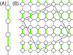
Figure 1: Cluster shapes of the (A) one- and (B) two-dimensional systems of interacting $S=1$ dimers. Our calculations have been carried out for $N=20$ in both cases. In (B), the tilted square of $\sqrt{20}\times\sqrt{20}$ is shown with dotted lines. The thick green and thin black bonds denote the intra- and interdimer interactions, respectively.

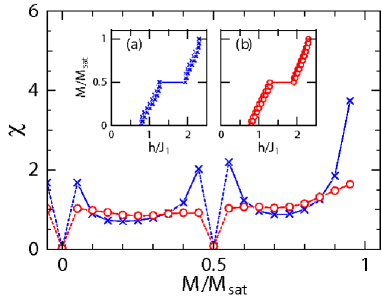
Figure 2: Field-derivative of the magnetization $\chi$ of the one- and two-dimensional systems of interacting $S=1$ dimers, denoted by crosses and circles, respectively. Insets (a) and (b) show the magnetization process of the one-dimensional case (A) in Fig. 1 for $J_{2}/J_{1}=0.15$ and that of the two-dimensional case (B) for $J_{2}/J_{1}=0.05$, respectively. The main panel shows $\chi$ as a function of the magnetization divided by the saturation with corresponding colors and symbols.

The Hamiltonian of the interacting $S=1$ dimers is given by

$${\cal H}=\sum_{\langle i,j\rangle}J_{1}\mbox{\boldmath$S$}_{i}\cdot\mbox{\boldmath$S$}_{j}+\sum_{\langle i,j\rangle}J_{2}\mbox{\boldmath$S$}_{i}\cdot\mbox{\boldmath$S$}_{j}+h\sum_{i}S^{z}_{i},$$ (2)

where $\mbox{\boldmath$S$}_{i}$ denotes the $S=1$ spin operator. Here, the first term describes the intradimer interactions (denoted by the thick green bonds in Fig. 1), the second term describes the interdimer interactions (denoted by the thin black bonds in Fig. 1), and the third term is the Zeeman term. Note that $J_{1}$ is the energy unit; thus, we set $J_{1}=1$. We examine the cases for the clusters depicted in Fig. 1. The results, which are depicted in Fig. 2, will help us accurately capture the behavior of $\chi$ near the magnetization plateau. The system size is $N=20$ commonly. In the two-dimensional case, the tilted square shown in Fig. 1 is treated. The magnetization processes of the one-dimensional case (A) for $J_{2}/J_{1}=0.15$ and the two-dimensional case (B) for $J_{2}/J_{1}=0.05$ are presented in insets (a) and (b) in Fig. 2, respectively. We choose these parameters so that the sum of the amplitudes of interdimer interactions operating a dimer of the thick green bond is the same in Figs. 1(A) and 1(B). We can clearly observe a plateau at $M/M_{\rm sat}=1/2$ in both cases. Note that the experimentally observed magnetization processes were reported for one-dimensional systems of Ni compounds[16, 17] and for the two-dimensional system of the organic biradical F₂PNNNO[18]. The one- and two-dimensional magnetization processes appear to be very similar; it is difficult to find a clear difference between them. Let us next discuss the behavior of $\chi$, the results for which are presented in the main panel. Near half the height of the saturation, we can observe that $\chi$ diverges in the one-dimensional system, while it remains finite in the two-dimensional system. These properties originate from the nature of the density of states determined from the parabolic dispersion. It is noticeable that the behavior does not change for each dimension, irrespective of the difference in the lower- or higher-field sides, and that the value of $\chi$ just at $M$ of the plateau is discontinuous with the values of $\chi$ around it. One can find that $\chi$ clearly exhibits the behavior of a typical magnetization plateau from the above observation. Note that these characteristics of $\chi$ appear not only at $M/M_{\rm sat}=1/2$ but also at $M=0$. The behavior at $M=0$ is already well known in various cases[19, 20, 21, 22]; the behavior of $\chi$ in these cases clearly satisfies the characteristics mentioned above.

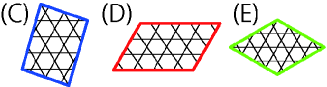
Figure 3: Shapes of the finite-size clusters in the kagome lattice. Cluster (C) is the same as that for $N=33$ in ref. References. Cluster (D) is the new cluster for $N=36$, while cluster (E) is that for $N=36$ in ref. References.

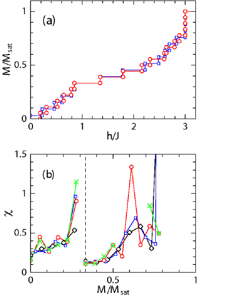
Figure 4: Results for the kagome-lattice antiferromagnets. (a) Magnetization processes shown for the $N=36$ cluster (D) and the $N=33$ cluster (C) with circles and squares, respectively. (b) Field-derivative of the magnetization $\chi$ as a function of the magnetization divided by the saturation. Circles and squares in (b) denote the results of $\chi$ corresponding to the cases in (a). Crosses correspond to the $N=36$ cluster (E). Note that part of $\chi$ for the $N=36$ cluster (E) is missing because $\chi$ cannot be defined when the lowest-energy state in the subspace does not become the ground state of the system in the magnetic field. Diamonds represent the case of the $N=30$ cluster investigated in ref. References.

We now examine the magnetization process of the kagome-lattice antiferromagnet. Its Hamiltonian is given by

$${\cal H}=\sum_{\langle i,j\rangle}J\mbox{\boldmath$S$}_{i}\cdot\mbox{\boldmath$S$}_{j}+h\sum_{i}S^{z}_{i},$$ (3)

where the sum of the first term runs over the nearest neighbors on the kagome lattice. Note that $\mbox{\boldmath$S$}_{i}$ in eq. (3) denotes the $S=1/2$ spin operator and that $J$ is the energy unit; thus, we set $J=1$. The shape of the finite-size cluster of the kagome lattice under the periodic boundary condition is not necessarily unique even when the number of spin sites $N$ is given. In fact, for $N=36$, there is another shape, denoted by the red cluster (D) in Fig. 3, which is different from that treated by Honecker et al. in ref. References; the cluster of Honecker et al. is shown in Fig. 3(E). In this letter, we present the result for the red cluster (D) for $N=36$, which helps us know the finite-size effects from the difference between the two cases (D) and (E) for $N=36$.

The result of the magnetization process of the red cluster (D) for $N=36$ sites is depicted in Fig. 4(a). We also give the full result of the blue cluster (C) for $N=33$, which is the same cluster as that treated by Hida in ref. References. In Fig. 4(b), we present the results of $\chi$ for the finite-size systems of $N=30$, 33, and 36. We focus our attention on the behavior of $\chi$ around $M/M_{\rm sat}\sim 1/3$. One can observe that around $M/M_{\rm sat}\sim 1/3$, shown in Fig. 4(b), $\chi$ exhibits divergent behavior on the smaller-$M$ side, while it is very small on the larger-$M$ side; namely, the behavior on the smaller-$M$ side is not the same as that on the larger-$M$ side. This fact is markedly different from the behavior of $\chi$ for the interacting $S=1$ dimer systems around $M/M_{\rm sat}\sim 1/2$ in Fig. 2. In particular, the divergent behavior on the smaller-$M$ side appears to be similar to that in the one-dimensional case even though the lattice is two-dimensional without any isotropy. This behavior may suggest that a one-dimensional spin structure forms in the two-dimensional lattice structure. A similar one-dimensional feature in the kagome lattice was reported in refs. References and References. The relationship between the present result and that in refs. References and References is an open problem which should be tackled in the near future. Since the divergent behavior appears on the smaller-$M$ side, the external field corresponding to $M/M_{\rm sat}\sim 1/3$ is the critical field. On the other hand, on the larger-$M$ side, there is no divergent behavior of $\chi$. It is noticeable that $\chi$ from the larger-$M$ side is continuous with $\chi$ just at $M/M_{\rm sat}=1/3$. It is unclear whether or not $\chi$ at $M/M_{\rm sat}=1/3$ vanishes as $N\rightarrow\infty$ at the present time.

From these observations, the behavior of the magnetization around $M/M_{\rm sat}=1/3$ is anomalous; it is reasonable to consider that the behavior is a new phenomenon in magnetization. The schematic behavior of $M$ around $M/M_{\rm sat}=1/3$ based on the discussion of the characteristics of $\chi$ is shown in Fig. 5. The shape is similar to the ramp of a Nordic ski jump when seen from the horizontally sideways direction. Thus, we call the behavior of $M$ a magnetization ramp. This behavior is markedly different from the magnetization process of a classical system on the kagome lattice[13]. Although the magnetization ramp may appear to be a magnetization cusp, the ramp is definitely different from a cusp because a conventional cusp occurs at the level crossing between two states with finite gradients, for example, as reported in ref. References. Thus, a magnetization ramp is an unusual and new phenomenon.

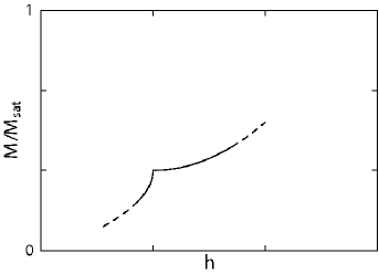
Figure 5: Schematic shape of the magnetization ramp.

Next, we discuss the characteristic behavior of other parts with respect to the relative height in our finite-size magnetization processes. We successfully observe a jump near the saturation, which was proven in ref. References. Note that several eigenstates with various values of $S_{z}^{\rm tot}$ degenerate just at $h/J=3$. In the $N=36$ magnetization process reported in ref. References, a jump appears at $M/M_{\rm sat}=11/18$; at the field where the lowest-energy eigenvalue in the subspace of $S_{z}^{\rm tot}=10$ meets that of $S_{z}^{\rm tot}=12$, the energy is lower than the lowest-energy eigenvalue in the subspace of $S_{z}^{\rm tot}=11$. In this meaning, this jump is different from the jump near the saturation discussed above. In the present result for $N=36$ in Fig. 4(a), however, the jump at $M/M_{\rm sat}=11/18$ does not appear. It is thus unclear whether or not the jump at this relative height survives in the thermodynamic limit. Even in these situations, when one focuses on the behavior of $\chi$ near $M/M_{\rm sat}\sim 0.6$ in Fig. 4(b), $\chi$ is enhanced irrespective of the system size except for the case of the green cluster (E) for $N=36$, in which $\chi$ cannot be obtained near $M/M_{\rm sat}\sim 0.6$; the enhancement suggests the existence of some anomaly around $M/M_{\rm sat}\sim 0.6$. It should be clarified in future studies whether this anomaly is a jump in the magnetization process or another.

Finally, let us discuss the relationship between our observation of the magnetization process of the ideal $S=1/2$ kagome-lattice Heisenberg antiferromagnet and the magnetization measurement of the actual compounds volborthite and vesignieite, which have relatively small values of $J$. These materials include other factors that are not considered in the ideal situation assumed in this study. Vesignieite includes a small amount of impurity spins according to the results of recent studies. In volborthite, on the other hand, there is spatial anisotropy in the bonds, although very pure samples are available. It should be noted that the magnetization processes of both materials reveal flat behavior at about $M/M_{\rm sat}\sim 0.4$[27], which is slightly larger than the (theoretical) numerical result of $M/M_{\rm sat}=1/3$. It should be investigated in the near future whether or not the missing factors mentioned above are the origin of this difference in height of $M$ exhibiting the flat behavior and whether or not these factors affect the appearance of the magnetization ramp. In particular, in ref. References it was reported that in volborthite, another anomalous behavior in its magnetization process is observed at around $M=(1/6)\mu_{\rm B}$/Cu and (1/45)$\mu_{\rm B}$/Cu, referred to as “magnetization steps.”[28] In the result for the red cluster (D) of $N=36$ in Fig. 4, small enhancements of $\chi$ appear at $M/M_{\rm sat}=1/6$ and 1/18. Unfortunately, the resolution is not sufficient to judge whether or not the finite-size data surely capture the behavior of the magnetization steps; calculations for larger systems are greatly anticipated.

In summary, we have examined the magnetization process of the $S=1/2$ kagome-lattice Heisenberg antiferromagnet from the viewpoint of its gradient $\chi$ based on numerical-diagonalization finite-size data. The observation of $\chi$ is very useful for extracting characteristics in the magnetization process that are difficult to detect when only the magnetization process is observed. Our observation leads to a new phenomenon, a magnetization ramp. To confirm the existence of the phenomenon, two approaches will be necessary in future studies. One of them is the construction of an effective theory. The other is a numerical examination of systems with larger sizes. We plan to carry out calculations for $N=39$; the results will be published elsewhere. In such works, something unknown in properties of kagome-lattice systems may be clarified further.

References

- [1] A brief history of the study on kagome-lattice magnetism was given in M. Mekata: Phys. Today 56 (2003) No.2, 12.
- [2] M. P. Shores, E. A. Nytko, B. M. Bartlett, and D. G. Nocera: J. Am. Chem. Soc. 127 (2005) 13462.
- [3] P. Mendels and F. Bert: J. Phys. Soc. Jpn. 79 (2010) 011001.
- [4] Y. Okamoto, H. Yoshida, and Z. Hiroi: J. Phys. Soc. Jpn. 78 (2009) 033701.
- [5] H. Yoshida, Y. Okamoto, T. Tayama, T. Sakakibara, M. Tokunaga, A. Matsuo, Y. Narumi, K. Kindo, M. Yoshida, M. Takigawa, and Z. Hiroi: J. Phys. Soc. Jpn. 78 (2009) 043704.
- [6] M. Yoshida, M. Takigawa, H. Yoshida, Y. Okamoto, and Z. Hiroi: Phys. Rev. Lett. 103 (2009) 077207.
- [7] T. Nakamura and S. Miyashita: Phys. Rev. B 52 (1995) 9174.
- [8] P. Lecheminant, B. Bernu, C. Lhuillier, L. Pierre, and P. Sindzingre: Phys. Rev. B 56 (1997) 2521.
- [9] Ch. Waldtmann, H.-U. Everts, B. Bernu, C. Lhuillier, P. Sindzingre, P. Lecheminant, and L. Pierre: Eur. Phys. J. B 2 (1998) 501.
- [10] O. Cepas, C. M. Fong, P. W. Leung, and C. Lhuillier: Phys. Rev. B 78 (2008) 140405(R).
- [11] P. Sindzingre and C. Lhuillier: Europhys. Lett. 88 (2009) 27009.
- [12] K. Hida: J. Phys. Soc. Jpn. 70 (2001) 3673.
- [13] D. C. Cabra, M. D. Grynberg, P. C. W. Holdsworth, and P. Pujol: Phys. Rev. B 65 (2002) 094418.
- [14] J. Schulenberg, A. Honecker, J. Schnack, J. Richter, and H.-J. Schmidt: Phys. Rev. Lett. 88 (2002) 167207.
- [15] A. Honecker, J. Schulenberg, and J. Richter: J. Phys.: Condens. Matter 16 (2004) S749.
- [16] Y. Narumi, M. Hagiwara, R. Sato, K. Kindo, H. Nakano, and M. Takahashi: Physica B 246-247 (1998) 509.
- [17] Y. Narumi, K. Kindo, M. Hagiwara, H. Nakano, A. Kawaguchi, K. Okunishi, and M. Kohno: Phys. Rev. B 69 (2004) 174405.
- [18] Y. Hosokoshi, Y. Nakazawa, K. Inoue, K. Takizawa, H. Nakano, M. Takahashi, and T. Goto: Phys. Rev. B 60 (1999) 12924.
- [19] M. Takahashi and T. Sakai: J. Phys. Soc. Jpn. 60 (1991) 760.
- [20] I. Affleck: Phys. Rev. B 43 (1991) 3215.
- [21] T. Sakai and M. Takahashi: Phys. Rev. B 57 (1998) R8091.
- [22] N. Katoh and M. Imada: J. Phys. Soc. Jpn. 63 (1994) 4529.
- [23] T. Ohashi, N. Kawakami, and H. Tsunetsugu: Phys. Rev. Lett. 97 (2006) 066401.
- [24] T. Ohashi, S. Suga, N. Kawakami, and H. Tsunetsugu: J. Phys.: Condens. Matter 19 (2007) 145251.
- [25] K. Okunishi and T. Tonegawa: J. Phys. Soc. Jpn. 72 (2003) 479.
- [26] M. E. Zhitomirsky and H. Tsunetsugu: Phys. Rev. B. 70 (2004) 100403.
- [27] Y. Okamoto: private communication.
- [28] The relative heights of the magnetization steps in ref. References are the consequence of the assumption that the -factor is 2. Note that the actual -factor is slightly different from [29].
- [29] H. Ohta, W. Zhang, S. Okubo, M. Tomoo, M. Fujisawa, H. Yoshida, Y. Okamoto, and Z. Hiroi: J. Phys.: Conf. Series 145 (2009) 012010.