Quantum Experimental Data in Psychology and Economics

Abstract

We prove a theorem which shows that a collection of experimental data of probabilistic weights related to decisions with respect to situations and their disjunction cannot be modeled within a classical probabilistic weight structure in case the experimental data contain the effect referred to as the ‘disjunction effect’ in psychology. We identify different experimental situations in psychology, more specifically in concept theory and in decision theory, and in economics (namely situations where Savage’s Sure-Thing Principle is violated) where the disjunction effect appears and we point out the common nature of the effect. We analyze how our theorem constitutes a no-go theorem for classical probabilistic weight structures for common experimental data when the disjunction effect is affecting the values of these data. We put forward a simple geometric criterion that reveals the non classicality of the considered probabilistic weights and we illustrate our geometrical criterion by means of experimentally measured membership weights of items with respect to pairs of concepts and their disjunctions. The violation of the classical probabilistic weight structure is very analogous to the violation of the well-known Bell inequalities studied in quantum mechanics. The no-go theorem we prove in the present article with respect to the collection of experimental data we consider has a status analogous to the well known no-go theorems for hidden variable theories in quantum mechanics with respect to experimental data obtained in quantum laboratories. For this reason our analysis puts forward a strong argument in favor of the validity of using a quantum formalism for modeling the considered psychological experimental data as considered in this paper.

1 Introduction

There exists an intensive ongoing research activity focusing on the use of the mathematical formalism of quantum mechanics to model situations in cognition and economics [1, 2, 3, 4]. Our group at the Leo Apostel Center in Brussels has played a role in the initiation of this research domain [5, 6, 7, 8, 9, 10, 11, 12, 13, 14], and is still actively engaged in it [15, 16, 17, 18, 19, 20, 21, 22].

In the present article we make use of insights and techniques developed in the foundations of quantum mechanics to investigate whether a specific collection of experimental data can be modeled by means of a classical theory, or whether a more general theory is needed, eventually a quantum theory. For decades intensive research has been conducted focussing on the very question, since physicists wanted to know whether quantum mechanics itself could be substituted by a classical theory. This body of research is traditionally referred to as ‘the hidden variable problem of quantum mechanics’, because indeed such a classical theory giving rise to the same predictions as quantum mechanics would be a theory containing ‘hidden variables’, to account for classical determinism on a hidden not necessarily manifest level. The presence of quantum-type probabilities would occur as a consequence of the lack of knowledge of these hidden variables on the manifest level. Physicists had already encountered such a situation before, namely classical statistical mechanics is a hidden variable theory for thermodynamics, i.e. the positions and velocities of the molecules of a given substance are hidden variables when the thermodynamic description level of the substance is the manifest level [23, 24, 25, 26, 27, 28, 29, 30, 31, 32, 33, 34, 35, 36, 37, 38, 39, 40, 42, 43, 44, 45, 46, 47]. John von Neumann proved the first no-go theorem for the existence of hidden variables for quantum mechanics [23], and this was followed by the famous Einstein-Podolsky-Rosen paradox proposal [24]. Critical investigations with respect to both von Neumann’s no-go theorem and the EPR paradox were performed by Bell [28, 30]. Then followed the proposal of an effective hidden variable theory, nowadays called ‘Bohm’s theory’, [29], elaborations of von Neumann’s theorem, i.e. further investigations from a structural perspective [26, 27, 31, 36, 38, 42, 43, 44, 45, 47], and extensive discussions about several aspects of the problem [32, 33, 34, 46]. In the seventies the experimentalist became interested, and this lead to new developments, e.g. the sharpening of notions such as locality, separability, etc…. But most of all, quantum mechanics was now confirmed as a profoundly reliable physical theory, even when scrutinized under all types of aspects where failure could be expected in a plausible way [35, 37, 39, 40]. In the eighties, it was shown, step by step, that by focusing on the mathematical structure of the probability model used to model experimental data, it was possible to distinguish between data that are quantum (more correctly ‘non-classical’, in the sense of not allowing a modeling within a classical Kolmogorovian probability model [41]), and data that are classical (hence can be modeled within a Kolmogorovian probability model) [38, 42, 43, 44, 45, 47]. One of the aspects of this hidden variable research, which from the foundations of quantum mechanics point of view is definitely of more universal importance and value, is that the results with respect to the characterization of a set of experimental data, i.e. whether these data can be modeled within a classical theory or not, do not depend on whether these data are obtained from measurements in a physics laboratory. For sets of data whether obtained from experiments in psychology or economics (or in any other domain of science) the same analysis can be made, and the same techniques of characterization of these data can be employed.

We have already investigated in this way data that were gathered by experiments measuring membership weights of an item with respect to two concepts and the conjunction of these two concepts [48]. These experimental data provide experimental evidence for a quantum structure in cognition [17]. The deviation of what a classical probability theory would provide in modeling these experimental data was called ‘overextension’ in concept research circles [48]. Many experiments by different concept researchers have measured the presence of ‘overextension’ for the conjunction of concepts [49, 50, 51, 52, 53, 54], such that the ‘deviation from classicality’ is experimentally well documented and abundant. There is a correspondence between ‘overextension’ for typicality and membership weight values for the conjunction of concept, and what in decision theory is referred to as ‘the conjunction fallacy’ [55, 56]. In the present article we want to concentrate on the ‘disjunction’, and ‘how deviations from classicality appear when the disjunction is at play’. The experimental data that we consider as our elements of study are the results of measurements of membership weights of items with respect to pairs of concepts and their disjunction [57]. In an analogous way like conjunction deviations from classicality in concept theories relate to the conjunction fallacy in decision theory, there is the well studied disjunction effect in decision theory which corresponds to these disjunction deviations in concept theories [58, 59, 60, 61, 62, 63, 64, 65, 66, 67, 68, 69]. In economics too, an effect similar to this disjunction effect was observed, more specifically in situations where Savage’s Sure-Thing Principle [70], a fundamental hypothesis of classical economic theory, is violated. We refer here to the Allais and Ellsberg paradoxes [71, 72].

Before putting forward a simple criterion and also a geometric interpretation of it in the next section, we would like to mention that the disjunction effect in decision theory has been modeled quantum mechanically by several authors [73, 74, 75]. The disjunction effect, as it appears for the membership weights of items with respect to pairs of concepts and their disjunction, was modeled explicitly by the quantum mechanical formalism in our Brussels group [14, 15, 19]. The result of the present article, namely that the disjunction effect cannot be modeled classically, supports the quantum models that have been put forward for it.

2 Classical and non classical membership weights for concepts

The ‘disjunction’ experiments we want to focus on in the present article were performed with the aim of measuring deviations for membership weights of items with respect to concepts from how one would expect such membership weights to behave classically [57]. For example, the concepts Home Furnishings and Furniture and their disjunction ‘Home Furnishings or Furniture’ are considered. With respect to this pair, the item Ashtray is considered. Subjects rated the membership weight of Ashtray for the concept Home Furnishings as 0.7 and the membership weight of the item Ashtray for the concept Furniture as 0.3. However, the membership weight of Ashtray with respect to the disjunction ‘Home Furnishings or Furniture’ was rated as only 0.25, i.e. less than either one of the weights assigned for both concepts separately. This means that subjects found Ashtray to be ‘less strongly a member of the disjunction ‘Home Furnishings or Furniture’ than they found it to be a member of the concept Home Furnishings alone or a member of the concept Furniture alone’. If one thinks intuitively about the ‘logical’ meaning of a disjunction, then this is an unexpected result. Indeed, if somebody finds that Ashtray belongs to Home Furnishings, they would be expected to also believe that Ashtray belongs to ‘Home Furnishings or Furniture’. The same holds for Ashtray and Furniture. Hampton called this deviation (this relative to what one would expect according to a standard classical interpretation of the disjunction) ‘underextension’ [57].

A typical experiment testing the effect described above proceeds as follows. The tested subjects are asked to choose a number from the following set: $\{-3,-2,-1,0,$ $+1,+2,+3\}$, where the positive numbers +1, +2 or +3 mean that they consider ‘the item to be a member of the concept’ and the typicality of the membership increases with an increasing number. Hence +3 means that the subject who attributes this number considers the item to be a very typical member, and +1 means that he or she considers the item to be a not so typical member. The negative numbers indicate non-membership, again in increasing order, i.e. -3 indicates strong non-membership, and -1 represents weak non-membership. Choosing 0 indicates the subject is indecisive about the membership or non-membership of the item. Subjects were asked to repeat the procedure for all the items and concepts considered. Membership weights were then calculated by dividing the number of positive ratings by the number of non-zero ratings.

Considering again the case of Ashtray as an item and its membership with respect to the concepts Home Furnishings and Furniture and their disjunction. As the experiments are conceived, each individual subject will decide for Ashtray whether it is a member or not a member of respectively Home Furnishings, Furniture and ‘Home Furnishings or Furniture’. Suppose that there are $n$ subjects participating in the experiment. There is a way to express what we mean intuitively by ‘classical behavior’. Indeed, what we would ‘not’ like to happen is that a subject, decides Ashtray to be a member of Home Furnishings, but not a member of Home Furnishings or Furniture. If a subject would make such type of decision, then this would be in direct conflict with the meaning of the disjunction. However, in the case of Ashtray, since $0.7\times n$ subjects have decided that Ashtray is a member of Home Furnishings and only $0.25\times n$ subjects have decided it to be a member of ‘Home Furnishings or Furniture’, this means that at least $0.55\times n$ subjects have taken this decision in direct conflict with the meaning of the disjunction. In case $n=100$, this means $55$ subjects (more than half) have done so.

Suppose we introduce the following notation, and indicate with $A_{1}$ the first considered concept, hence Home Furnishings, and with $\mu(A_{1})$ the membership weight of item $X$, hence Ashtray, with respect to $A_{1}$. This means that for our example we have $\mu(A_{1})=0.7$. With $A_{2}$ we denote the second considered concept, hence Furniture, and with $\mu(A_{2})$ the membership weight of item $X$, hence Ashtray, with respect to $A_{2}$. This means that for our example we have $\mu(A_{2})=0.3$. With ‘$A_{1}$ or $A_{2}$’ we denote the disjunction of both concepts $A_{1}$ and $A_{2}$, hence ‘Home Furnishings or Furniture’, and with $\mu(A_{1}\ {\rm or}\ A_{2})$ the membership weight of item $X$, hence Ashtray, with respect to ‘$A_{1}$ or $A_{2}$’.

We can easily see that the non classical effect we analyzed above cannot happen in case the following two inequalities are satisfied

$$\mu(A_{1})\leq\mu(A_{1}\ {\rm or}\ A_{2})$$ (1)

$$\mu(A_{2})\leq\mu(A_{1}\ {\rm or}\ A_{2})$$ (2)

and we observe indeed that both inequalities are violated for our example of Ashtray with respect to Home Furnishings and Furniture.

There is another issue which we do not want to happen, and this one is somewhat more subtle. To illustrate it, we consider another example of the experiments, namely the item Olive, with respect to the pair of concepts Fruits and Vegetables and their disjunction ‘Fruits or Vegetables’. The respective membership weights were measured to be $\mu(A_{1})=0.5$, $\mu(A_{2})=0.1$ and $\mu(A_{1}\ {\rm or}\ A_{2})=0.8$. Obviously inequalities (1) and (2) are both satisfied for this example. Let us suppose again that there are $n$ subjects participating in the experiment. Then $0.5\times n$ subjects have decided that Olive is a member of Fruits, and $0.1\times n$ subjects have decided that Olive is a member of Vegetables, while $0.8\times n$ subjects have decided that Olive is a member of ‘Fruits or Vegetables’. However, at maximum $0.5\times n+0.1\times n=0.6\times n$ subjects have decided that Olive is a member of Fruits ‘or’ is a member of Vegetables. This means that a minimum of $0.4\times n$ subjects have decided that Olive is neither a member of Fruits nor a member of Vegetables. But $0.8\times n$ subjects have decided that Olive is a member of ‘Fruits or Vegetables’. This means that a minimum of $0.2\times n$ subjects have decided that Olive ‘is not’ a member of Fruits, and also ‘is not’ a member of Vegetables, but ‘is’ a member of ‘Fruits or Vegetables’. The decision made by these $0.2\times n$ subjects, hence 20 in case $n=100$, goes directly against the meaning of the disjunction. An item becoming a member of the disjunction while it is not a member of both pairs is completely non classical. We can easily see that this second type of non classicality cannot happen in case the following inequality is valid

$$\mu(A_{1}\ {\rm or}\ A_{2})\leq\mu(A_{1})+\mu(A_{2})$$ (3)

and indeed this inequality is violated by the example of Olive with respect to Fruits and Vegetables. One of the authors has derived in earlier work the three inequalities (1), (2) and (3) as a consequence of a different type of requirement, namely the requirement that the membership weights are in their most general form representations of mathematical normed measures (see section 1.4, Theorem 4 and Appendix B of [15], and Theorem 4.1 of the present article). The items that deviated from classicality by violating one or both of the inequalities (1) and (2) were called $\Delta$-type non classical items. The items that deviated from classicality by violating inequality (3) were called $k$-type non classical items. An explicit quantum model was constructed for both types of non classical items [15]. In the present paper we consider the general situation of $n$ concepts and disjunctions of pairs of these $n$ concepts, and we introduce the corresponding definition for classicality. We will additionally derive a simple geometrical criterion to verify whether the membership weights of an item with respect to a set of concepts and disjunctions of pairs of them can be modeled classically or not. Table 1 represents the items and pairs of concepts tested by Hampton [57] which we will use as experimental data to illustrate the analysis put forward in the present article.

We consider $n$ concepts $A_{1},A_{2},\ldots,A_{n}$ and membership weights $\mu(A_{i})$ of an item $X$ with respect to each concept $A_{i}$, and also membership weights $\mu(A_{i}\ \mathrm{or}\ A_{j})$ of this item $X$ with respect to the disjunction of concepts $A_{i}$ and $A_{j}$. It is not necessary that membership weights of the item $X$ are determined with respect to each one of the possible pairs of concepts. Hence, to describe this situation formally, we consider a set $S$ of pairs of indices $S\subseteq\{(i,j)\ |\ i<j;i,j=1,2,\ldots,n\}$ corresponding to those pairs of concepts for which the membership weights of the item $X$ have been measured with respect to the disjunction of these pairs. Hence, the following set of membership weights have been experimentally determined

$$p_{i}=\mu(A_{i})\quad i=1,2,\ldots,n;\quad p_{i\vee j}=\mu(A_{i}\ \mathrm{or}\ A_{j})\quad(i,j)\in S$$ (4)

Definition 2.1 (Classical Disjunction Data)

We say that the set of membership weights of an item $X$ with respect to concepts is a ‘classical disjunctive set of membership weights’ if it has a normed measure representation. Hence if there exists a normed measure space $(\Omega,\sigma(\Omega),P)$ with $E_{A_{1}},E_{A_{2}},\ldots,E_{A_{n}}\in\sigma(\Omega)$ elements of the event algebra, such that

$$p_{i}=P(E_{A_{i}})\quad i=1,2,\ldots,n;\quad p_{i\vee j}=P(E_{A_{i}}\cup E_{A_{j}})\quad(i,j)\in S$$ (5)

A normed measure $P$ is a function defined on a $\sigma$-algebra $\sigma(\Omega)$ over a set $\Omega$ and taking values in the interval $[0,1]$ such that the following properties are satisfied: (i) The empty set has measure zero, i.e. $P(\emptyset)=0$; (ii) Countable additivity or $\sigma$-additivity: if $E_{1}$, $E_{2}$, $E_{3}$, $\dots$ is a countable sequence of pairwise disjoint sets in $\sigma(\Omega)$, the measure of the union of all the $E_{i}$ is equal to the sum of the measures of each $E_{i}$, i.e. $P(\bigcup_{i=1}^{\infty}E_{i})=\sum_{i=1}^{\infty}P(E_{i})$; (iii) The total measure is one, i.e. $P(\Omega)=1$. The triple $(\Omega,\sigma(\Omega),P)$ is called a normed measure space, and the members of $\sigma(\Omega)$ are called measurable sets. A $\sigma$-algebra over a set $\Omega$ is a

Table 1: The eight pairs of concepts and items of experiment 2 in [57]. $\mu(A_{1})$, $\mu(A_{2})$ and $\mu(A_{1}{\rm or}A_{2})$ are respectively the measured membership weights of each item with respect to the concepts $A_{1}$, $A_{2}$ and their disjunction $A_{1}$or$A_{2}$. The non classical items are labeled by $q$ and the classical items by $c$.

		$\mu(A_{1})$	$\mu(A_{2})$	$\mu(A_{1}{\rm or}A_{2})$			$\mu(A_{1})$	$\mu(A_{2})$	$\mu(A_{1}{\rm or}A_{2})$
$A_{1}$=Home Furnishing, $A_{2}$=Furniture					$A_{1}$=Spices, $A_{2}$=Herbs
Mantelpiece	$q$	0.8	0.4	0.75	Molasses	$c$	0.4	0.05	0.425
Window Seat	$q$	0.9	0.9	0.8	Salt	$q$	0.75	0.1	0.6
Painting	$q$	0.9	0.5	0.85	Peppermint	$c$	0.45	0.6	0.6
Light Fixture	$q$	0.8	0.4	0.775	Curry	$q$	0.9	0.4	0.75
Kitchen Count	$q$	0.8	0.55	0.625	Oregano	$q$	0.7	1	0.875
Bath Tub	$c$	0.5	0.7	0.75	MSG	$q$	0.15	0.1	0.425
Desk Chair	$c$	0.1	0.3	0.35	Chili Pepper	$q$	1	0.6	0.95
Shelves	$c$	1	0.4	1	Mustard	$q$	1	0.8	0.85
Rug	$c$	0.9	0.6	0.95	Mint	$c$	1	0.8	0.925
Bed	$c$	1	1	1	Cinnamon	$c$	1	0.4	1
Wall-Hangings	$c$	0.9	0.4	0.95	Parsley	$c$	0.5	0.9	0.95
Space Rack	$q$	0.7	0.5	0.65	Saccharin	$q$	0.1	0.01	0.15
Ashtray	$q$	0.7	0.3	0.25	Poppyseeds	$c$	0.4	0.4	0.4
Bar	$q$	0.35	0.6	0.55	Pepper	$c$	0.9	0.6	0.95
Lamp	$q$	1	0.7	0.9	Turmeric	$q$	0.7	0.45	0.675
Wall Mirror	$q$	1	0.6	0.95	Sugar	$q$	0	0	0.2
Door Bell	$c$	0.5	0.1	0.55	Vinegar	$q$	0.1	0.01	0.35
Hammock	$q$	0.2	0.5	0.35	Sesame Seeds	$c$	0.35	0.4	0.625
Desk	$c$	1	1	1	Lemon Juice	$q$	0.1	0.01	0.15
Refrigerator	$q$	0.9	0.7	0.575	Chocolate	$c$	0	0	0
Park Bench	$q$	0	0.3	0.05	Horseradish	$q$	0.2	0.4	0.7
Waste Paper Basket	$q$	1	0.5	0.6	Vanilla	$q$	0.6	0	0.275
Sculpture	$c$	0.8	0.4	0.8	Chires	$q$	0.6	1	0.95
Sink Unit	$q$	0.9	0.6	0.6	Root Ginger	$q$	0.7	0.15	0.675
$A$=Hobbies, $B$=Games					$A$=Instruments, $B$=Tools
Gardening	$c$	1	0	1	Broom	$q$	0.1	0.7	0.6
Theatre-Going	$c$	1	0	1	Magnetic Compass	$c$	0.9	0.5	1
Archery	$q$	1	0.9	0.95	Tuning Fork	$c$	0.9	0.6	1
Monopoly	$c$	0.7	1	1	Pen-Knife	$q$	0.65	1	0.95
Tennis	$c$	1	1	1	Rubber Band	$q$	0.25	0.5	0.25
Bowling	$c$	1	1	1	Stapler	$c$	0.85	0.8	0.85
Fishing	$c$	1	0.6	1	Skate Board	$q$	0.1	0	0
Washing Dishes	$q$	0.1	0	0.15	Scissors	$q$	0.85	1	0.9
Eating Ice-Cream Cones	$q$	0.2	0	0.1	Pencil Eraser	$q$	0.4	0.7	0.45
Camping	$q$	1	0.1	0.9	Tin Opener	$c$	0.9	0.9	0.95
Skating	$q$	1	0.6	0.95	Bicycle Pump	$q$	1	0.9	0.7
Judo	$q$	1	0.7	0.8	Scalpel	$q$	0.8	1	0.925
Guitar Playing	$c$	1	0	1	Computer	$q$	0.6	0.8	0.6
Autograph Hunting	$q$	1	0.2	0.9	Paper Clip	$q$	0.3	0.7	0.6
Discus Throwing	$q$	1	0.75	0.7	Paint Brush	$c$	0.65	0.9	0.95
Jogging	$q$	1	0.4	0.9	Step Ladder	$q$	0.2	0.9	0.85
Keep Fit	$q$	1	0.3	0.95	Door Key	$q$	0.3	0.1	0.95
Noughts	$q$	0.5	1	0.9	Measuring Calipers	$q$	0.9	1	0.9
Karate	$q$	1	0.7	0.8	Toothbrush	$c$	0.4	0.4	0.5
Bridge	$c$	1	1	1	Sellotape	$q$	0.1	0.2	0.325
Rock Climbing	$q$	1	0.2	0.95	Goggles	$q$	0.2	0.3	0.15
Beer Drinking	$q$	0.8	0.2	0.575	Spoon	$q$	0.65	0.9	0.7
Stamp Collecting	$c$	1	0.1	1	Pliers	$c$	0.8	1	1
Wrestling	$q$	0.9	0.6	0.625	Meat Thermometer	$c$	0.75	0.8	0.9

		$\mu(A_{1})$	$\mu(A_{2})$	$\mu(A_{1}{\rm or}A_{2})$			$\mu(A_{1})$	$\mu(A_{2})$	$\mu(A_{1}{\rm or}A_{2})$
$A_{1}$=Pets, $A_{2}$=Farmyard Animals					$A_{1}$=Fruits, $A_{2}$=Vegetables
Goldfish	$q$	1	0	0.95	Apple	$c$	1	0	1
Robin	$c$	0.1	0.1	0.1	Parsley	$q$	0	0.2	0.45
Blue-Tit	$c$	0.1	0.1	0.1	Olive	$q$	0.5	0.1	0.8
Collie Dog	$c$	1	0.7	1	Chili Pepper	$c$	0.05	0.5	0.5
Camel	$q$	0.4	0	0.1	Broccoli	$q$	0	0.8	1
Squirrel	$q$	0.2	0.1	0.1	Root Ginger	$q$	0	0.3	0.55
Guide Dog for the Blind	$q$	0.7	0	0.9	Pumpkin	$c$	0.7	0.8	0.925
Spider	$c$	0.5	0.35	0.55	Raisin	$q$	1	0	0.9
Homing Pig	$q$	0.9	0.1	0.8	Acorn	$q$	0.35	0	0.4
Monkey	$q$	0.5	0	0.25	Mustard	$q$	0	0.2	0.175
Circus Horse	$q$	0.4	0	0.3	Rice	$q$	0	0.4	0.325
Prize Bull	$q$	0.1	1	0.9	Tomato	$c$	0.7	0.7	1
Rat	$q$	0.5	0.7	0.4	Coconut	$q$	0.7	0	1
Badger	$q$	0	0.25	0.1	Mushroom	$q$	0	0.5	0.9
Siamese Cat	$q$	1	0.1	0.95	Wheat	$q$	0	0.1	0.2
Race Horse	$c$	0.6	0.25	0.65	Green Pepper	$c$	0.3	0.6	0.8
Fox	$q$	0.1	0.3	0.2	Watercress	$q$	0	0.6	0.8
Donkey	$q$	0.5	0.9	0.7	Peanut	$c$	0.3	0.1	0.4
Field Mouse	$q$	0.1	0.7	0.4	Black Pepper	$c$	0.15	0.2	0.225
Ginger Tom-Cat	$q$	1	0.8	0.95	Garlic	$q$	0.1	0.2	0.5
Husky in Sledream	$q$	0.4	0	0.425	Yam	$c$	0.45	0.65	0.85
Cart Horse	$q$	0.4	1	0.85	Elderberry	$q$	1	0	0.8
Chicken	$q$	0.3	1	0.95	Almond	$q$	0.2	0.1	0.425
Doberman Guard Dog	$q$	0.6	0.85	0.8	Lentils	$q$	0	0.6	0.525
$A$=Sportswear, $B$=Sports Equipment					$A$=Household Appliances, $B$=Kitchen Utensils
American Foot	$c$	1	1	1	Fork	$q$	0.7	1	0.95
Referee’s Whistle	$q$	0.6	0.2	0.45	Apron	$c$	0.3	0.4	0.5
Circus Clowns	$q$	0	0	0.1	Hat Stand	$q$	0.45	0	0.3
Backpack	$c$	0.6	0.5	0.6	Freezer	$q$	1	0.6	0.95
Diving Mask	$q$	1	1	0.95	Extractor Fan	$q$	1	0.4	0.9
Frisbee	$q$	0.3	1	0.85	Cake Tin	$c$	0.4	0.7	0.95
Sunglasses	$q$	0.4	0.2	0.1	Carving Knife	$c$	0.7	1	1
Suntan Lotion	$q$	0	0	0.1	Cooking Stove	$c$	1	0.5	1
Gymnasium	$q$	0	0.9	0.825	Iron	$q$	1	0.3	0.95
Motorcycle Helmet	$q$	0.7	0.9	0.75	Food Processor	$c$	1	1	1
Rubber Flipper	$c$	1	1	1	Chopping Board	$q$	0.45	1	0.95
Wrist Sweat	$q$	1	1	0.95	Television	$q$	0.95	0	0.85
Golf Ball	$c$	0.1	1	1	Vacuum Cleaner	$c$	1	0	1
Cheerleaders	$c$	0.3	0.4	0.45	Rubbish Bin	$c$	0.5	0.5	0.8
Linesman’s Flag	$q$	0.1	1	0.75	Vegetable Rack	$c$	0.4	0.4	0.7
Underwater	$q$	1	0.65	0.6	Broom	$c$	0.55	0.4	0.625
Baseball Bat	$c$	0.2	1	1	Rolling Pin	$c$	0.45	1	1
Bathing Costume	$q$	1	0.8	0.8	Table Mat	$q$	0.25	0.4	0.325
Sailing Life Jacket	$c$	1	0.8	1	Whisk	$c$	1	1	1
Ballet Shoes	$q$	0.7	0.6	0.6	Blender	$c$	1	1	1
Hoola Hoop	$q$	0.1	0.6	0.5	Electric Toothbrush	$q$	0.8	0	0.55
Running Shoes	$c$	1	1	1	Frying Pan	$q$	0.7	1	0.95
Cricket Pitch	$q$	0	0.5	0.525	Toaster	$c$	1	1	1
Tennis Racket	$c$	0.2	1	1	Spatula	$c$	0.55	0.9	0.95

nonempty collection $\sigma(\Omega)$ of subsets of $\Omega$ that is closed under complementation and countable unions of its members. Measure spaces are the most general structures devised by mathematicians and physicists to represent weights.

3 Geometrical characterization of membership weights

We now develop the geometric language that makes it possible to verify the existence of a normed measure representation for a set of weights. For this purpose we introduce the ‘classical disjunction polytope’ $d_{c}\left(n,S\right)$ in the following way. We construct an $n+\left|S\right|$ dimensional ‘classical disjunction vector’

$$\overrightarrow{p}=\left(p_{1},p_{2},\ldots,p_{n},\ldots,p_{i\vee j},\ldots\right)$$

where $|S|$ is the cardinality of $S$. We consider the linear space $R\left(n,S\right)\cong\mathbb{R}^{n+\left|S\right|}$ consisting of all real vectors of this type. Next, let $\varepsilon\in\left\{0,1\right\}^{n}$ be an arbitrary $n$-dimensional vector consisting of $0$ and $1$’s. For each $\varepsilon$ we construct the classical disjunction vector $\overrightarrow{v}^{\varepsilon}\in R\left(n,S\right)$ by putting:

$$\begin{array}[]{cc}v_{i}^{\varepsilon}=\varepsilon_{i}&i=1,\ldots,n\\ v_{ij}^{\varepsilon}=\max\left(\varepsilon_{i},\varepsilon_{j}\right)=\varepsilon_{i}+\varepsilon_{j}-\varepsilon_{i}\varepsilon_{j}&\left(i,j\right)\in S\end{array}$$

The set of convex linear combinations of $\overrightarrow{v}^{\varepsilon}$ we call the ‘classical disjunction polytope’ $d_{c}\left(n,S\right):$

$$d_{c}\left(n,S\right)=\left\{\overrightarrow{w}\in R\left(n,S\right)\mid\overrightarrow{w}=\underset{\varepsilon\in\left\{0,1\right\}^{n}}{\sum}\lambda_{\varepsilon}\overrightarrow{v}^{\varepsilon};\lambda_{\varepsilon}\geq 0;\underset{\varepsilon\in\left\{0,1\right\}^{n}}{\sum}\lambda_{\varepsilon}=1\right\}$$

We prove now the following theorem

Theorem 3.1

The set of weights

$$p_{i}=\mu(A_{i})\quad i=1,2,\ldots,n;\quad p_{i\vee j}=\mu(A_{i}\ \mathrm{or}\ A_{j})\quad(i,j)\in S$$

admits a normed measure space, and hence is a classical disjunction set of membership weights, if and only if its disjunction vector $\overrightarrow{p}$ belongs to the classical disjunction polytope $d_{c}\left(n,S\right)$.

Proof: Suppose that (4) is a classical disjunction set of weights, and hence we have a normed measure space $(\Omega,\sigma(\Omega),P)$ and events $E_{A_{i}}\in\sigma(\Omega)$ such that (5) are satisfied. Let us show that in this case $\overrightarrow{p}\in d_{c}\left(n,S\right)$. For an arbitrary subset $X\subset\Omega$ we define $X^{1}=X$ and $X^{0}=\Omega\backslash X$. Consider $\epsilon=(\epsilon_{1},\ldots,\epsilon_{n})\in\{0,1\}^{n}$ and define $A(\epsilon)=\cap_{\epsilon}A_{i}^{\epsilon_{i}}$. Then we have that $A(\epsilon)\cap A(\epsilon^{\prime})=\emptyset$ for $\epsilon\not=\epsilon^{\prime}$, $\cup_{\epsilon}A(\epsilon)=\Omega$, and $\cup_{\epsilon,\epsilon_{j}=1}A(\epsilon)=A_{j}$. We put now $\lambda_{\epsilon}=P(A(\epsilon))$. Then we have $\lambda_{\epsilon}\geq 0$ and $\sum_{\epsilon}\lambda_{\epsilon}=1$, and $p_{i}=P(A_{i})=\sum_{\epsilon,\epsilon_{i}=1}\lambda_{\epsilon}=\sum_{\epsilon}\lambda_{\epsilon}\epsilon_{i}$. We also have $p_{i\vee j}=P(A_{i}\cup A_{j})=\sum_{\epsilon,\max\left(\epsilon_{i},\epsilon_{j}\right)=1}\lambda_{\epsilon}=\sum_{\epsilon}\lambda_{\epsilon}\left(\epsilon_{i}+\epsilon_{j}-\epsilon_{i}\epsilon_{j}\right)$. This means that $\overrightarrow{p}=\sum_{\epsilon}\lambda_{\epsilon}v^{\epsilon}$, which shows that $\overrightarrow{p}\in d_{c}\left(n,S\right)$. Conversely, suppose that $\overrightarrow{p}\in d_{c}\left(n,S\right)$. Then there exist numbers $\lambda_{\epsilon}\geq 0$ such that $\sum_{\epsilon}\lambda_{\epsilon}=1$ and $\overrightarrow{p}=\sum_{\epsilon}\lambda_{\epsilon}v^{\epsilon}$. We define $\Omega=\{0,1\}^{n}$ and $\sigma(\Omega)$ the power set of $\Omega$. For $X\subset\Omega$ we define then $P(X)=\sum_{\epsilon\in X}\lambda_{\epsilon}$. Then we choose $A_{i}=\{\epsilon,\epsilon_{i}=1\}$ which gives that $P(A_{i})=\sum_{\epsilon}\lambda_{\epsilon}\epsilon_{i}=\sum_{\epsilon}\lambda_{\epsilon}v_{i}^{\epsilon}=p_{i}$ and $P(A_{i}\cup A_{j})=\sum_{\epsilon}\lambda_{\epsilon}\left(\epsilon_{i}+\epsilon_{j}-\epsilon_{i}\epsilon_{j}\right)=\sum_{\epsilon}\lambda_{\epsilon}v_{ij}^{\epsilon}=p_{i\vee j}$. This shows that we have a classical disjunction set of weights. QED

As one may notice, these results are very similar to those of Pitowsky for classical conjunction polytopes $c\left(n,S\right)$ [47]. However, the Pitowsky correlation polytope and the classical disjunction polytope have different sets of vertices. Furthermore, the interpretation of the $|S|$ components is completely different, namely representing conjunction data $p_{ij}$ and disjunction data $p_{i\vee j}$ respectively. In general, the existence of a classical disjunctive representation does not necessarily imply the existence of a classical conjunctive representation, and vice versa. Therefore, in order to fully grasp classicality by these geometric means, the natural next step is to combine the theoretical results for conjunction (Pitowsky) and disjunction polytopes (developed here and in [15]) by introducing a ‘classical connective polytope’.

Again, let $\varepsilon\in\left\{0,1\right\}^{n}$ be an arbitrary $n$-dimensional vector consisting of $0$ and $1$’s. For each $\varepsilon$ we construct the classical connective vector $\overrightarrow{w}^{\varepsilon}\in\mathbb{R}^{n+\left|S\right|+\left|S^{\prime}\right|}$ by putting:

$$\begin{array}[]{cc}w_{i}^{\varepsilon}=\varepsilon_{i}&i=1,\ldots,n\\ w_{ij}^{\varepsilon}=\varepsilon_{i}\varepsilon_{j}=\min\left(\varepsilon_{i},\varepsilon_{j}\right)&\left(i,j\right)\in S\\ w_{k\vee l}^{\varepsilon}=\varepsilon_{k}+\varepsilon_{l}-\varepsilon_{k}\varepsilon_{l}=\max\left(\varepsilon_{k},\varepsilon_{l}\right)&\left(k,l\right)\in S^{\prime}\end{array}$$

The set of convex linear combinations of $\overrightarrow{w}^{\varepsilon}$ we call the ‘classical connective polytope’ $k(n,S,S^{\prime})$:

$$k(n,S,S^{\prime})=\{\overrightarrow{f}\in\mathbb{R}^{n+\left|S\right|+\left|S^{\prime}\right|}\ |\ \overrightarrow{f}=\sum_{\epsilon\in\{0,1\}^{n}}\lambda_{\epsilon}\overrightarrow{w}^{\epsilon};\ \lambda_{\epsilon}\geq 0;\ \sum_{\epsilon\in\{0,1\}^{n}}\lambda_{\epsilon}=1\}$$ (6)

Theorem 3.2

The set of weights

$$p_{i}=\mu(A_{i})\quad i=1,2,\ldots,n;\quad p_{ij}=\mu(A_{i}\ \mathrm{and}\ A_{j})\quad(i,j)\in S;p_{i\vee j}=\mu(A_{i}\ \mathrm{or}\ A_{j})\quad(i,j)\in S^{\prime}$$

admits a normed measure space, and hence is a classical set of membership weights, if and only if its connective vector $\overrightarrow{p}$ belongs to the classical connective polytope $k(n,S,S^{\prime}).$

Proof: Follows from the theorems for conjunction and disjunction classicality.

4 A simple case: disjunction effect for 2 concepts

One of the authors studied the disjunction effect for the case of two concepts and their disjunction [15]. We recall Theorem 4 of [15].

Theorem 4.1

The membership weights $\mu(A),\mu(B)$ and $\mu(A\ \mathrm{or}\ B)$ of an item $X$ with respect to concepts $A$ and $B$ and their disjunction ‘$A$ or $B$’ are classical disjunction data if and only if they satisfy the following ‘classical disjunction’ inequalities:

$$0\leq\mu(A)\leq\mu(A\ \mathrm{or}\ B)\leq 1$$ (7)

$$0\leq\mu(B)\leq\mu(A\ \mathrm{or}\ B)\leq 1$$ (8)

$$0\leq\mu(A)+\mu(B)-\mu(A\ \mathrm{or}\ B)$$ (9)

Proof: See [15].

In the case of two concepts $A_{1}$, $A_{2}$ and their disjunction ‘$A_{1}\ \mathrm{or}\ A_{2}$’ the set of indices is $S=\{(1,2)\}$ and the classical disjunction polytope $d_{c}\left(n,S\right)$ is contained in the $2+|S|=3$ dimensional Euclidean space, i.e. $R(2,\{1,2\})={\mathbb{R}}^{3}$. Furthermore we have four vectors $\epsilon\in\{0,1\}^{n}$, namely $(0,0),(0,1),(1,0)$ and $(1,1)$, and hence the four vectors $\overrightarrow{v}^{\epsilon}\in{\mathbb{R}}^{3}$ which are the following

$$\overrightarrow{v}^{(0,0)}=(0,0,0)\quad\overrightarrow{v}^{(1,0)}=(1,0,1)\quad\overrightarrow{v}^{(0,1)}=(0,1,1)\quad\overrightarrow{v}^{(1,1)}=(1,1,1)$$ (10)

This means that the correlation polytope $d_{c}\left(n,S\right)$ is the convex region spanned by the convex combinations of the vectors $(0,0,0),(1,0,1),(0,1,1)$ and $(1,1,1)$, and the disjunction vector is given by $\overrightarrow{p}=(\mu(A_{1}),\mu(A_{2}),\mu(A_{1}\ \mathrm{or}\ A_{2}))$. It is well-known that every polytope admits two dual descriptions: one in terms of convex combinations of its vertices, and one in terms of the inequalities that define its boundaries. Following [15], the inequalities defining the boundaries for the polytope $d_{c}\left(2,\{(1,2)\}\right)$ are given by:

$$0\leq p_{1}\leq p_{1\vee 2}\leq 1$$ (11)

$$0\leq p_{2}\leq p_{1\vee 2}\leq 1$$ (12)

$$0\leq p_{1}+p_{2}-p_{1\vee 2}\leq 1$$ (13)

We observe that the last inequality $p_{1}+p_{2}-p_{1\vee 2}\leq 1$ follows easily because from $p_{1}\leq p_{1\vee 2}$ and $p_{2}\leq p_{1\vee 2}$ follows that $p_{1}+p_{2}-p_{1\vee 2}\leq p_{1\vee 2}\leq 1$ (again because of (11)).

Theorem 4.2

The classical disjunction inequalities formulated in theorem 4.1. are satisfied if and only if $\overrightarrow{p}\in d_{c}\left(2,\{(1,2)\}\right).$

Proof: Let us notice that

$$\overrightarrow{p} = \left(\begin{array}[]{c}p_{1}\\ p_{2}\\ p_{1\vee 2}\end{array}\right)=\left(1-p_{1\vee 2}\right)\left(\begin{array}[]{c}0\\ 0\\ 0\end{array}\right)+\left(p_{1\vee 2}-p_{1}\right)\left(\begin{array}[]{c}0\\ 1\\ 1\end{array}\right)+\left(p_{1\vee 2}-p_{2}\right)\left(\begin{array}[]{c}1\\ 0\\ 1\end{array}\right)+\left(p_{1}+p_{2}-p_{1\vee 2}\right)\left(\begin{array}[]{c}1\\ 1\\ 1\end{array}\right)$$

$$= a\left(\begin{array}[]{c}0\\ 0\\ 0\end{array}\right)+b\left(\begin{array}[]{c}0\\ 1\\ 1\end{array}\right)+c\left(\begin{array}[]{c}1\\ 0\\ 1\end{array}\right)+d\left(\begin{array}[]{c}1\\ 1\\ 1\end{array}\right)$$

Hence if the classical disjunction inequalities formulated in theorem 4.1 are satisfied, then it is easy to check that $\overrightarrow{p}\in d_{c}\left(2,\{(1,2)\}\right).$Vice versa, let $\overrightarrow{p}\in d_{c}\left(2,\{(1,2)\}\right).$ Rewriting $\overrightarrow{p}$ as above, and putting condition $0\leq a,b,c,d\leq 1$ immediately follow the classical disjunction inequalities of theorem 4.1:

$$\begin{array}[]{c}0\leq 1-p_{1\vee 2}\leq 1\\ 0\leq p_{1\vee 2}-p_{1}\leq 1\\ 0\leq p_{1\vee 2}-p_{2}\leq 1\\ 0\leq p_{1}+p_{2}-p_{1\vee 2}\leq 1\end{array}$$

The last inequality is condition (13), while $0\leq 1-p_{1\vee 2}\Rightarrow p_{1\vee 2}\leq 1.$ Also $0\leq p_{1\vee 2}-p_{1}\Rightarrow p_{1}\leq p_{1\vee 2}.$ Also, $0\leq p_{1}+p_{2}-p_{1\vee 2}$ implies that $p_{1\vee 2}-p_{2}\leq p_{1}$ and since $0\leq p_{1\vee 2}-p_{2}$ follows that $0\leq p_{1\vee 2}-p_{2}\leq p_{1}$ so $0\leq p_{1}.$ Putting these together, we obtain then $0\leq p_{1}\leq p_{1\vee 2}\leq 1.$ Similarly, we can prove $0\leq p_{2}\leq p_{1\vee 2}\leq 1.$ QED.

Let us consider the experimental data in Table 1. In the first part of Figure 1 we have represented the disjunction vectors formed by the membership weights of the different items to be found in Table 1 with respect to the pairs of concepts Home Furnishings and Furniture and their disjunction ‘Home Furnishings or Furniture’, and also the disjunction polytope. The classical items, hence with disjunction vector inside the polytope, are represented by a little open disk. They are Desk, Bed, Rug, Wall-Hangings, Shelves, Sculpture, Bath Tub, Door Bell and Desk Chair. The non classical items, hence with disjunction vector outside of the polytope, are represented by a little closed disk. They are Lamp, Wall Mirror, Window Seat, Painting, Light Fixture, Mantelpiece, Refrigerator, Space Rack, Sink Unit, Waste Paper Basket, Kitchen Count, Bar, Hammock, Ashtray and Park Bench.

In the second part of Figure 1 we have represented the disjunction vectors formed by the membership weights of the different items found in Table 1 with respect to the pairs of concepts Spices and Herbs and their disjunction ‘Spices or Herbs’, and the disjunction polytope. The classical items, hence with disjunction vector inside the polytope, are again represented by a little open disk. They are Parsley, Mint, Pepper, Cinnamon, Peppermint, Sesame Seeds, Poppyseeds, Molasses and Chocolate. The non classical items, hence with disjunction vector outside of the polytope, are again represented by a little closed disk. They are Chires, Oregano, Chili Pepper, Mustard, Horseradish, Turmeric, Root Ginger, Salt, Curry, MSG, Vinegar, Vanilla, Lemon Juice, Sugar and Saccharin.

In the first part of Figure 2 we have represented the disjunction vectors formed by the membership weights of the different items to be found in Table 1 with respect to the pairs of concepts Hobbies and Games and their disjunction ‘Hobbies or Games’, and also the disjunction polytope. The classical items, hence with disjunction vector inside the polytope, are represented by a little open disk. They are Monopoly, Tennis, Bridge, Bowling, Fishing, Theatre Going, Gardening and Guitar Playing. The non classical items, hence with disjunction vector outside of the polytope, are represented by a little closed disk. They are Noughts, Archery, Skating, Karate, Judo, Keep Fit, Jogging, Autograph Hunting, Discuss Throwing, Rock Climbing, Camping, Stamp Collection, Wrestling, Beer Drinking, Washing Dishes and Eating Ice-Cream Cones.

In the second part of Figure 2 we have represented the disjunction vectors formed by the membership weights of the different items found in Table 1 with respect to the pairs of concepts Games and Instruments and their disjunction ‘Games or Instruments’, and the disjunction polytope. The classical items, hence with disjunction vector inside the polytope, are represented by a little open disk. They are Pliers, Tin Opener, Paint Brush, Meat Thermometer, Tuning Fork, Stapler, Magnetic Compass and Toothbrush. The non classical items, hence with disjunction vector outside of the polytope, are represented by a little closed disk. They are Pen-Knife, Scalpel, Scissors, Bicycle Pump, Step Ladder, Spoon, Door Key, Measuring Calipers, Paper Clip, Computer, Pencil Eraser, Broom, Sellotape, Rubber Band, Goggles and Skate Board.

In the first part of Figure 3 we have represented the disjunction vectors formed by the membership weights of the different items to be found in Table 1 with respect to the pairs of concepts Pets and Farmyard Animals and their disjunction ‘Pets or Farmyard Animals’, and also the disjunction polytope. The classical items, hence with disjunction vector inside the polytope, are represented by a little open disk. They are Colie Dog, Race Horse, Spider, Robin and Blue Tit. The non classical items, hence with disjunction vector outside of the polytope, are represented by a little closed disk. They are Chicken, Ginger Tom-Cat, Prize Bull, Cart Horse, Donkey, Doberman Guard Dog, Siamese Cat, Goldfish, Rat, Guide Dog fro the Blind, Homing Pig, Field Mouse, Fox, Husky in Sledream, Badger, Circus Horse, Monkey, Squirrel and Camel.

In the second part of Figure 3 we have represented the disjunction vectors formed by the membership weights of the different items found in Table 1 with respect to the pairs of concepts Fruits and Vegetables and their disjunction ‘Fruits or Vegetables’, and the disjunction polytope. The classical items, hence with disjunction vector inside the polytope, are again represented by a little open disk. They are Pumpkin, Tomato, Yam, Green Pepper, Apple, Chili Pepper, Peanut and Black Pepper. The non classical items, hence with disjunction vector outside of the polytope, are again represented by a little closed disk. They are Broccoli, Mushroom, Watercress, Coconut, Raisin, Olive, Elderberry, Lentils, Root Ginger, Garlic, Parsley, Almond, Rice, Acorn, Wheat and Mustard.

In the first part of Figure 4 we have represented the disjunction vectors formed by the membership weights of the different items to be found in Table 1 with respect to the pairs of concepts Sportswear and Sports Equipment and their disjunction ‘Sportswear or Sports Equipment’, and also the disjunction polytope. The classical items, hence with disjunction vector inside the polytope, are represented by a little open disk. They are Golf Ball, Tennis Racket, Baseball Bat, American Foot, Rubber Flipper, Running Shoes, Sailing Life Jacket, Backpack and Cheerleaders. The non classical items, hence with disjunction vector outside of the polytope, are represented by a little closed disk. They are Diving Mask, Wrist Sweat, Frisbee, Gymnasium, Lineman’s Flag, Ballet Shoes, Motorcycle Helmet, Bathing Costume, Underwater, Hoola Hoop, Cricket Pitch, Referee’s Whistle, Sunglasses, Circus Clowns and Suntan Lotion.

In the second part of Figure 4 we have represented the disjunction vectors formed by the membership weights of the different items found in Table 1 with respect to the pairs of concepts Household Appliances and Kitchen Utensils and their disjunction ‘Household Appliances or Kitchen Utensils’, and the disjunction polytope. The classical items, hence with disjunction vector inside the polytope, are again represented by a little open disk. They are Rolling Pin, Carving Knife, Whisk, Food Processor, Blender, Toaster, Spatula, Cake Tin, Cooking Stove, Rubbish Bin, Vacuum Cleaner, Vegetable Rack, Broom and Apron. The non classical

Figure 1: The polytopes for the concepts Home Furnishing and Furniture and the concepts Spices and Herbs. The classical items correspond to an open disk while the quantum ones to a full disk.

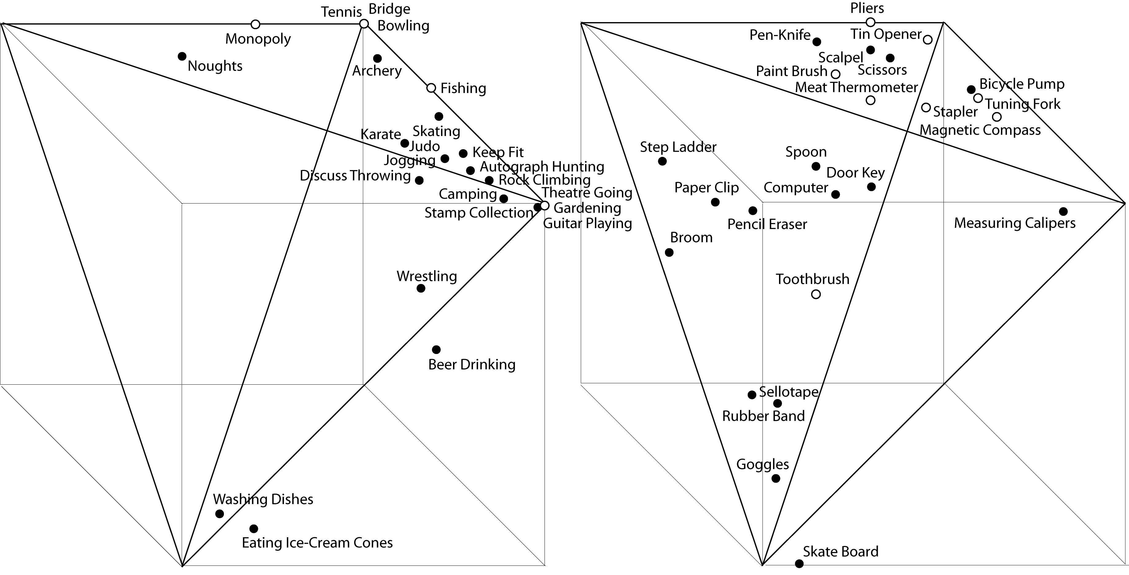
Figure 2: The polytopes for the concepts Hobbies and Games and the concepts Instruments and Tools. The classical items correspond to an open disk while the quantum ones to a full disk.

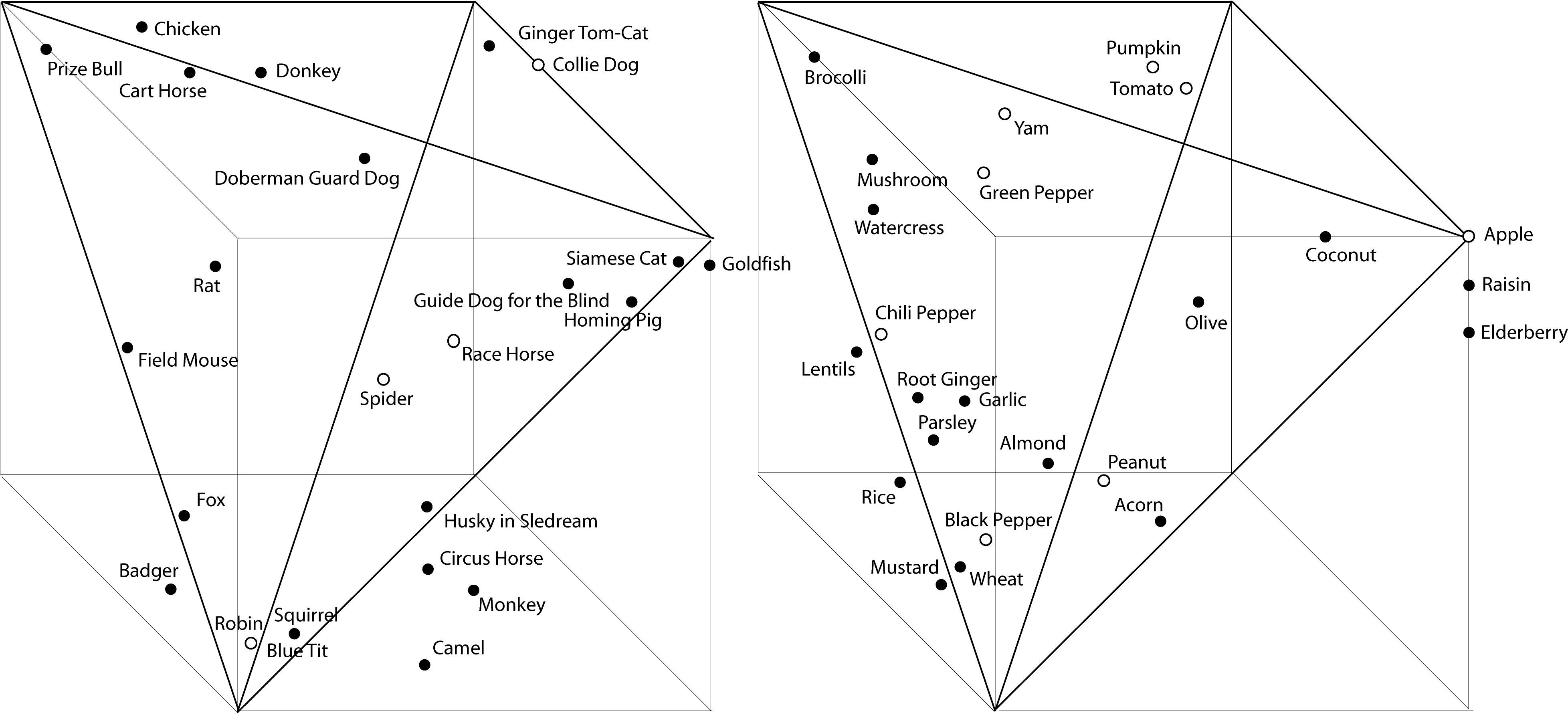
Figure 3: The polytopes for the concepts Pets and Farmyard Animals and the concepts Fruits and Vegetables. The classical items correspond to an open disk while the quantum ones to a full disk.

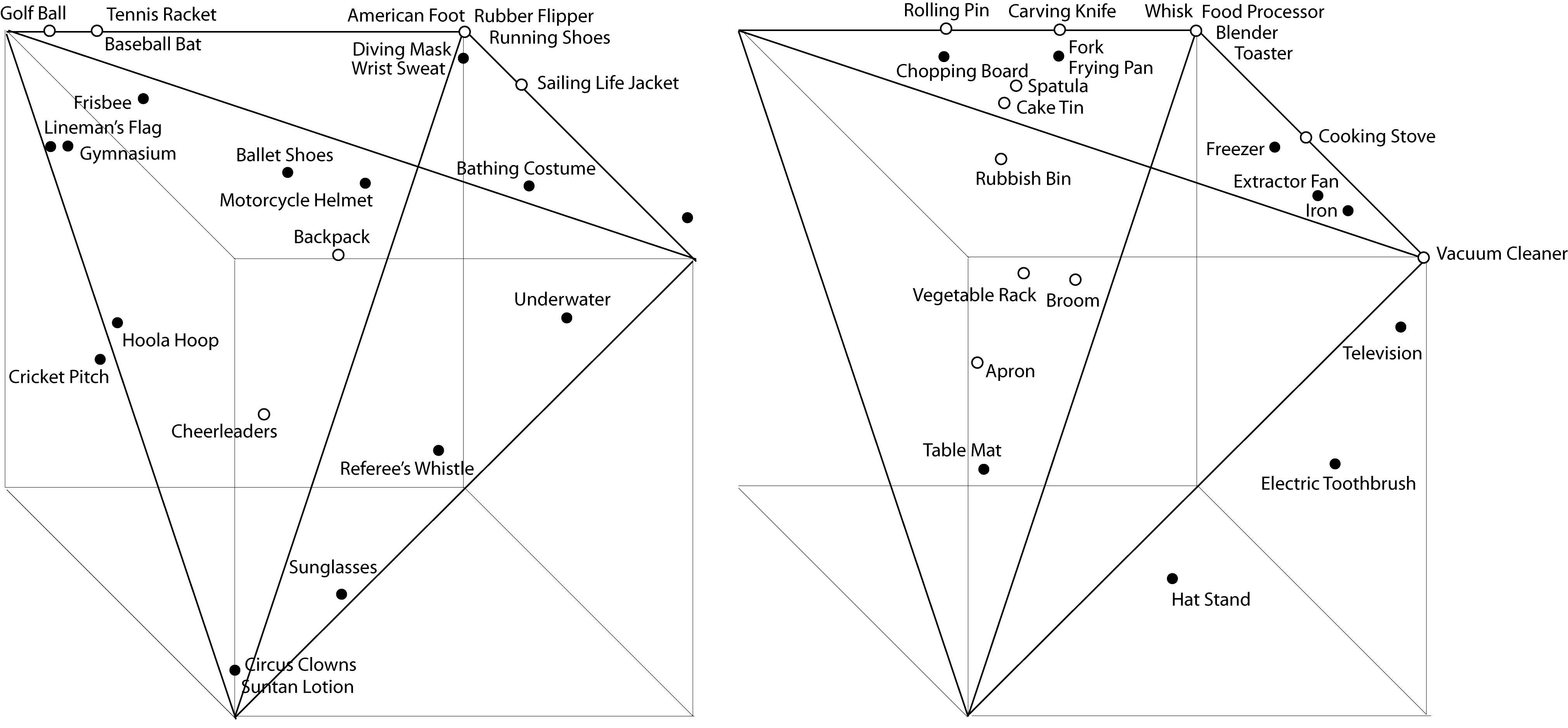
Figure 4: The polytopes for the concepts Sportswear and Sports Equipment and the concepts Household Appliances and Kitchen Utensils. The classical items correspond to an open disk while the quantum ones to a full disk.

items, hence with disjunction vector outside of the polytope, are again represented by a little closed disk. They are Fork, Frying Pan, Chopping Board, Freezer, Extractor Fan, Iron, Television, Electric Toothbrush, Table Mat and Hat Stand.

Remark that if the experimental data turn out such that the item is a classical item, this does not mean that perhaps non classical effect are at play also for this item. But the non classical effect might be such that they do not show up with these particular measurements. This aspect of the situation is analyzed in more detail in [15].

The inequalities that define the boundaries of polytope $d_{c}\left(n,S\right)$ are a variant of the well-known Bell inequalities [28, 47], studied in the foundations of quantum mechanics, but now put into the context of disjunctive connectives instead of conjunctive correlations. This means that the violation of these inequalities, such as it happens by the data corresponding to items for which the points lie outside the polytope, has from a probabilistic perspective an analogous meaning as the violation of Bell inequalities for the conjunction. Hence these violations may indicate the presence of quantum structures in the domain where the data is collected, which makes it plausible that a quantum model, such as for example the one proposed in [15], can be used to model the data.

As we have shown above, the classical disjunction polytope allows for one necessary and sufficient condition $\overrightarrow{p}\in d_{c}\left(n,S\right)$ which guarantees a classical Kolmogorovian model for the given set of probabilities to exist [41]. As illustrated here, this can be expressed by a set of Bell-like inequalities. However, as Pitowsky remarked [47], the number and complexity of the inequalities will grow so fast with $n$, that it would require exponentially many computation steps to derive them all. Anyway, already for the simplest (non-trivial) case $n=2$ interesting inequalities can be derived by which the non classical nature of a set of statistical data can be demonstrated explicitly. Such data exists in various fields of science: of course in quantum mechanics, but also in cognition (concept) theory, decision theory and some paradoxical situations in economics, such as in the Allais and Ellsberg paradox situations [71, 72], notably situations which violate Savage’s ‘Sure-Thing principle’ [70].

Acknowledgments

This work was supported by grants G.0405.08 and G.0234.08 of the Research Program of the Research Foundation-Flanders (FWO, Belgium).

References

- [1] Bruza, P. D. and Gabora, L. (Eds.) (2009). Special Issue: Quantum Cognition. Journal of Mathematical Psychology, 53, pp. 303-452.
- [2] Bruza, P. D., Lawless, W., Rijsbergen, C.J. van, Sofge, D. (Eds.) (2007). Proceedings of the AAAI Spring Symposium on Quantum Interaction. March 26-28, 2007. Stanford University, SS-07-08, AAAI Press.
- [3] Bruza, P. D., Lawless, W., Rijsbergen, C.J. van, Sofge, D., Coecke, B. and Clark, S. (Eds.) (2008). Proceedings of the Second Quantum Interaction Symposium. University of Oxford, March 26-28, 2008. London: College Publications.
- [4] Bruza, P. D., Sofge, D., Lawless, W., Rijsbergen, C.J. van, Klusch, M. (Eds.) (2009). Proceedings of the Third International Symposium, QI 2009, Saarbrücken, Germany, March 25-27, 2009, Lecture Notes in Computer Science Volume 5494. Berlin Heidelberg: Springer.
- [5] Aerts, D. and Aerts, S. (1994). Applications of quantum statistics in psychological studies of decision processes. Foundations of Science, 1, pp. 85-97; reprinted in B. C. van Fraassen (Ed.), Topics in the Foundation of Statistics, Springer, Dordrecht.
- [6] Aerts, D., Broekaert, J. and Smets, S. (1999). The liar paradox in a quantum mechanical perspective. Foundations of Science, 4, pp. 115-132.
- [7] Aerts, D., Broekaert, J., Smets, S. (1999). A quantum structure description of the liar paradox. International Journal of Theoretical Physics, 38, pp. 3231-3239.
- [8] Aerts, D., Aerts, S., Broekaert, J. and Gabora, L. (2000). The violation of Bell inequalities in the macroworld. Foundations of Physics, 30, pp. 1387-1414.
- [9] Gabora, L. and Aerts, D. (2002). Contextualizing concepts using a mathematical generalization of the quantum formalism. Journal of Experimental and Theoretical Artificial Intelligence, 14, pp. 327-358.
- [10] Aerts, D. and Czachor, M. (2004). Quantum aspects of semantic analysis and symbolic artificial intelligence. Journal of Physics A-Mathematical and General, 37, pp. L123-L132.
- [11] Aerts, D. and Gabora, L. (2005). A theory of concepts and their combinations I: The structure of the sets of contexts and properties. Kybernetes, 34, pp. 167-191.
- [12] Aerts, D. and Gabora, L. (2005). A theory of concepts and their combinations II: A Hilbert space representation. Kybernetes, 34, pp. 192-221.
- [13] Broekaert, J., Aerts, D. and D’Hooghe, B. (2006). The generalised Liar Paradox: A quantum model and interpretation. Foundations of Science, 11, pp. 399-418.
- [14] Aerts, D. (2007). General quantum modeling of combining concepts: A quantum field model in Fock space. Archive address and link: http://arxiv.org/abs/0705.1740.
- [15] Aerts, D. (2009). Quantum structure in cognition. Journal of Mathematical Psychology, 53, pp. 314-348.
- [16] Aerts, D. (2009). Quantum particles as conceptual entities: A possible explanatory framework for quantum theory. Foundations of Science, 14, pp. 361-411.
- [17] Aerts, D., Aerts, S. and Gabora, L. (2009). Experimental evidence for quantum structure in cognition. In P. D. Bruza, D. Sofge, W. Lawless, C. J. van Rijsbergen and M. Klusch (Eds.), Proceedings of QI 2009-Third International Symposium on Quantum Interaction, Book series: Lecture Notes in Computer Science, 5494, pp. 59-70. Berlin, Heidelberg: Springer.
- [18] Aerts, D. and D’Hooghe, B. (2009). Classical logical versus quantum conceptual thought: Examples in economics, decision theory and concept theory. In P. D. Bruza, D. Sofge, W. Lawless, C. J. van Rijsbergen and M. Klusch (Eds.), Proceedings of QI 2009-Third International Symposium on Quantum Interaction, Book series: Lecture Notes in Computer Science, 5494, pp. 128-142. Berlin, Heidelberg: Springer.
- [19] Aerts, D. (2010). Quantum interference and superposition in cognition: Development of a theory for the disjunction of concepts. In D. Aerts, B. D’Hooghe and N. Note (Eds.), Worldviews, Science and Us: Bridging Knowledge and Its Implications for Our Perspectives of the World. Singapore: World Scientific.
- [20] Aerts, D. (2010). Interpreting quantum particles as conceptual entities. International Journal of Theoretical Physics.
- [21] Aerts, D., Broekaert, J. and Gabora, L. (2010). A case for applying an abstracted quantum formalism to cognition. New Ideas in Psychology.
- [22] Aerts, D. and D’Hooghe, B. (2010). A quantum-conceptual explanation of violations of expected utility in economics. International Journal of Theoretical Physics.
- [23] von Neumann, J. (1932). Mathematische Grundlagen der Quantenmechanik. Berlin: Springer, Berlin. Chapter IV.1,2.
- [24] Einstein, A., Podolsky, B. and Rosen, N. (1935). Can quantum-mechanical description of physical reality be considered complete?, Physical Review, 47, pp. 777-780.
- [25] Bohr, N. (1935). Can quantum-mechanical description of physical reality be considered complete? Physical Review, 48, pp. 696-702.
- [26] Gleason, A. M. (1957). Measures on the closed subspaces of a Hilbert space. Journal of Mathematics and Mechanics, 6, pp. 885 893.
- [27] Jauch, J., and Piron, C. (1963). Can hidden variables be excluded from quantum mechanics? Helvetica Physica Acta, 36, pp. 827-837.
- [28] Bell, J. S. (1964). On the Einstein Podolsky Rosen Paradox, Physics, 1, pp. 195-200.
- [29] Bohm, D. and Bub, J. (1966). A proposed solution of the measurement problem in quantum mechanics by a hidden variable theory. Reviews of Modern Physics, 38, pp. 453-469.
- [30] Bell, J. S. (1966). On the problem of hidden variables in quantum mechanics, Reviews of Modern Physics, 38, pp. 447-452.
- [31] Kochen, S. and Specker, E. P. (1967). The problem of hidden variables in quantum mechanics. Journal of Mathematics and Mechanics, 17, pp. 59-87.
- [32] Jauch, J. M. and Piron, C. (1968). Hidden variables revisited. Reviews of Modern Physics, 40, pp. 228-229.
- [33] Gudder, S. P. (1968). Hidden variables in quantum mechanics reconsidered. Reviews of Modern Physics, 40, pp. 229-231.
- [34] Bohm, D. and Bub, J. (1968). On hidden variables-A reply to comments by Jauch and Piron and by Gudder. Reviews on Modern Physics, 40, pp. 235-236.
- [35] Clauser, J. F., Horne, M. A., Shimony, A. and Holt, R. A. (1969). Proposed experiment to test local hidden-variable theories, Physical Review Letters, 23, pp. 880-884.
- [36] Gudder, S. P. (1970). On hidden variable theories. Journal of Mathematical Physics, 11, pp. 431-436.
- [37] Clauser, J.F. and Horne, M.A. (1974). Experimental consequences of objective local theories, Physical Review D, 10, pp. 526-535.
- [38] Accardi, L. and Fedullo, A. (1982). On the statistical meaning of complex numbers in quantum mechanics. Lettere Al Nuovo Cimento, 34, pp. 161-172.
- [39] Aspect, A., Grangier, P. and Roger, G. (1982). Experimental realization of Einstein-Podolsky-Rosen-Bohm Gedankenexperiment: A new violation of Bell’s Inequalities. Physical Review Letters, 49, pp. 91-94.
- [40] Aspect, A., Dalibard, J. and Roger, G (1982). Experimental test of Bell’s Inequalities using time-varying analyzers. Physical Review Letters, 49, pp. 1804-1807.
- [41] Kolmogorov, A. N. (1956). Foundations of the Theory of Probability. New York: Chelsea Publishing Company.
- [42] Accardi L. (1984). The probabilistic roots of the quantum mechanical paradoxes. In S. Diner, D. Fargue, G. Lochak and F. Selleri (Eds.), The Wave-Particle Dualism: A Tribute to Louis de Broglie on his 90th Birthday (pp. 297-330). Dordrecht: Springer.
- [43] Aerts, D. (1985). A possible explanation for the probabilities of quantum mechanics and a macroscopical situation that violates Bell inequalities. In P. Mittelstaedt and E. W. Stachow (Eds.), Recent Developments in Quantum Logic, Grundlagen der Exacten Naturwissenschaften, vol.6, Wissenschaftverlag (pp. 235-251). Mannheim: Bibliographisches Institut.
- [44] Aerts, D. (1986). A possible explanation for the probabilities of quantum mechanics. Journal of Mathematical Physics,27, pp. 202-210.
- [45] Aerts, D. (1987). The origin of the non-classical character of the quantum probability model. In A. Blanquiere, S. Diner and G. Lochak (Eds.), Information, Complexity, and Control in Quantum Physics (pp. 77-100). Wien-New York: Springer-Verlag.
- [46] Redhead, M. (1987). Incompleteness, Nonlocality and Realism. Clarendon Press.
- [47] Pitowsky, I.( 1989). Quantum Probability, Quantum Logic. Lecture Notes in Physics 321. Heidelberg: Springer.
- [48] Hampton, J. A. (1988). Overextension of conjunctive concepts: Evidence for a unitary model for concept typicality and class inclusion. Journal of Experimental Psychology: Learning, Memory, and Cognition, 14, pp. 12-32.
- [49] Hampton, J. A. (1987). Inheritance of attributes in natural concept conjunctions. Memory & Cognition, 15, pp. 55-71.
- [50] Hampton, J. A. (1991). The combination of prototype concepts. In P. Schwanen ugel (Ed.), The Psychology of Word Meanings. Hillsdale, NJ: Erlbaum.
- [51] Storms, G., De Boeck, P., Van Mechelen, I. and Geeraerts, D. (1993). Dominance and non-commutativity e?ects in concept conjunctions: Extensional or intensional basis? Memory & Cognition, 21, pp. 752-762.
- [52] Hampton, J.A. (1996). Conjunctions of visually-based categories: overextension and compensation. Journal of Experimental Psychology: Learning, Memory and Cognition, 22, pp. 378-396.
- [53] Hampton, J. A. (1997). Conceptual combination: Conjunction and negation of natural concepts. Memory & Cognition, 25, pp. 888-909.
- [54] Storms, G., de Boeck, P., Hampton, J.A. and van Mechelen, I. (1999). Predicting conjunction typicalities by component typicalities. Psychonomic Bulletin and Review, 6, pp. 677-684.
- [55] Tversky, A. and Kahneman, D. (1982). Judgments of and by representativeness. In D. Kahneman, P. Slovic and A. Tversky (Eds.), Judgment under Uncertainty: Heuristics and Biases. Cambridge, UK: Cambridge University Press.
- [56] Tversky, A. and Kahneman, D. (1983). Extension versus intuitive reasoning: The conjunction fallacy in probability judgment. Psychological Review, 90, pp. 293-315.
- [57] Hampton, J. A. (1988). Disjunction of natural concepts. Memory & Cognition, 16, pp. 579-591.
- [58] Carlson, B. W. and Yates, J. F. (1989). Disjunction errors in qualitative likelihood judgment. Organizational Behavior and Human Decision Processes 44, pp. 368-379.
- [59] Tversky, A. and Shafir, E. (1992). The disjunction effect in choice under uncertainty. Psychological Science, 3, pp. 305-309.
- [60] Bar-Hillel, M. and Neter, E. (1993). How alike is it versus how likely is it: A disjunction fallacy in probability judgments. Journal of Personality and Social Psychology, 65, pp. 1119-1131.
- [61] Croson, R. T. A. (1999). The disjunction effect and reason-based choice in games. Organizational Behavior and Human Decision Processes, 80, pp. 118-133.
- [62] Kühberger, A., Komunska, D. and Perner, J. (2001). The disjunction effect: Does it exist for two-step gambles? Organizational Behavior and Human Decision Processes, 85, pp. 250-264.
- [63] Li, S. and Taplin, J. E. (2002). Examining whether there is a disjunction effect in prisoner’s dilemma games. Chinese Journal of Psychology, 44, pp. 25-46.
- [64] van Dijk, E. and Zeelenberg, M. (2003). The discounting of ambiguous information in economic decision making. Journal of Behavioral Decision Making, 16, pp. 341-352.
- [65] van Dijk, E. and Zeelenberg, M. (2006). The dampening effect of uncertainty on positive and negative emotions. Journal of Behavioral Decision Making, 19, pp. 171-176.
- [66] Bauer, M. I. and Johnson-Laird, P. N. (2006). How diagrams can improve reasoning. Psychological Science,4, pp. 372-378.
- [67] Lambdin, C. and Burdsal, C. (2007). The disjunction effect reexamined: Relevant methodological issues and the fallacy of unspecified percentage comparisons. Organizational behavior and human decision processes. Organizational behavior and human decision processes, 103, pp. 268-276.
- [68] Bagassi, M. and Macchi, L. (2007). The ‘vanishing’ of the disjunction effect by sensible procrastination. Mind & Society, 6, pp. 41-52.
- [69] Hristova, E. and Grinberg, M. (2008). Disjunction effect in prisoner’s dilemma: Evidences from an eye-tracking study. Cogsci 2008, Washington, July 22-26, proceedings.
- [70] Savage, L.J. (1954). The Foundations of Statistics. New-York: Wiley.
- [71] Allais, M. (1953). Le comportement de l’homme rationnel devant le risque: critique des postulats et axiomes de l’école Américaine. Econometrica, 21, pp. 503-546.
- [72] Ellsberg, D. (1961). Risk, ambiguity, and the Savage Axioms. Quarterly Journal of Economics, 75, pp. 643-669.
- [73] Busemeyer, J. R., Wang, Z. and Townsend J. T. (2006). Quantum dynamics of human decision-making. Journal of Mathematical Psychology, 50, pp. 220-241.
- [74] Pothos, E. M. and Busemeyer, J. R. (2009). A quantum probability explanation for violations of ‘rational’ decision theory. Proceedings of the Royal Society B.
- [75] Khrennikov, A. and Haven, E. (2009). Quantum mechanics and violations of the sure-thing principle: The use of probability interference and other concepts. Journal of Mathematical Psychology, 53, pp. 378-388.