Radially extended kinematics and stellar populations of the massive ellipticals NGC1600, NGC4125 and NGC7619.

We present high quality long slit spectra along the major and minor axes out to 1.5-2 $R_{e}$ (14-22 kpc) of three bright elliptical galaxies (NGC1600, NGC4125, NGC7619) obtained at the Hobby-Eberly Telescope (HET). We derive stellar kinematic profiles and Lick/IDS indices ($H\beta,Mgb,Fe_{5015},Fe_{5270},Fe_{5335},Fe_{5406}$). Moreover, for NGC4125 we derive gas kinematics and emission line strengths. We model the absorption line strengths using Simple Stellar Populations models that take into account the variation of $[\alpha/Fe]$ and derive ages, total metallicity and element abundances. Overall, we find that the three galaxies have old and $[\alpha/Fe]$ overabundant stellar populations with no significant gradients. The metallicity is supersolar at the center with a strong negative radial gradient. For NGC4125, several pieces of evidence point to a recent dissipational merger event. We calculate the broad band color profiles with the help of SSP models. All of the colors show sharp peaks at the center of the galaxies, mainly caused by the metallicity gradients, and agree well with the measured colors. Using the Schwarzschild’s axisymmetric orbit superposition technique, we model the stellar kinematics to constrain the dark halos of the galaxies. We use the tight correlation between the Mgb strength and local escape velocity to set limits on the extent of the halos by testing different halo sizes. Logarithmic halos – cut at 60 kpc – minimize the overall scatter of the Mgb-$V_{esc}$ relation. Larger cutoff radii are found if the dark matter density profile is decreasing more steeply at large radii.

1 Introduction

One of the most important remaining questions in contemporary astrophysics concerns the formation and evolution of stellar populations in elliptical galaxies. One can think of two globally different formation scenarios: the classic monolithic-collapse model for the formation and evolution of early-type galaxies (Tinsley 1972; Larson 1975; Tantalo et al. 1996) and the hierarchical merging scenario (White & Rees 1978; Kauffmann et al. 1993). In the former, early-type galaxies build most of their stars during a single event in the early universe while in the latter a substantial fraction of the stellar populations is formed from multiple mergers and the accretion of smaller objects over an extended period.

Statistically, the extremely small scatter of the observed color magnitude relation of elliptical galaxies or bright cluster members suggests that the stellar populations are surprisingly homogeneous (Bower et al. 1992; Kodama & Arimoto 1997). This uniformity of stellar populations in ellipticals is also supported by the internal tightness of the so called Fundamental Plane (Dressler et al. 1987; Djorgovski & Davis 1987; Bender et al. 1992; Saglia et al. 1993). These findings are consistent with a monolithic-collapse. Moreover, the tightness of the $Mg-\sigma$ relation for massive elliptical galaxies observed in the local universe (Bender et al. 1993; Sánchez-Blázquez et al. 2007) but holding up to the intermediate redshift $z\thickapprox 1$ (Ziegler & Bender 1997; Bender et al. 1998) requires a picture of a short, and highly efficient star formation process at high redshift and passive evolution since then.

In contrast, a large number of elliptical galaxies are observed to have kinematically decoupled cores and were explained as the result of dissipational major merging events by star dominated systems (Barnes 1992; Bender et al. 1989; Mehlert et al. 1998). Furthermore, boxy galaxies are mostly more massive, more radio-loud, more strong X-ray emitters, more frequently disturbed, and less flattened than disky early-type galaxies, suggesting that these two subclasses reflect different formation mechanisms and evolution history (Bender & Surma 1992; Nieto & Bender 1989). Recently, Kuntschner (2000); Thomas et al. (2005a); Collobert et al. (2006); Bernardi et al. (2006); Clemens et al. (2006); Rogers et al. (2010) showed that early-type galaxies in low density and in high density environments might exhibit different formation ages, and Sánchez-Blázquez et al. (2009); Matković et al. (2009) found evidence that lower mass galaxies have more extended star formation histories.

In standard closed-box models of chemical enrichment, the metallicity is a function of the yield and of how much gas has been locked after star formation has ceased (Tinsley 1980). Therefore, the metallicity strongly depends on the dynamical parameters – the deeper a potential is, the easier it is to retain gas in the galaxy. Then, galaxies formed in a monolithic-collapse should have steep radial metallicity gradients (Larson 1976; Thomas 1999), correlated with the local escape velocity – since the latter is a measure of the local depth of the potential well. On the other hand, major mergers, which come along with hierarchical merging will dilute stellar population gradients and their connection with the escape velocity as a result of violent relaxation (White 1980). In hierarchical merging, however, particularly for high-mass galaxies a significant amount of mass accretion can be due to minor mergers. If this deposites stellar populations that originally formed in small-mass halos preferentially in the outer parts of the final massive ellipticals, then this might enhance stellar-population gradients and one would again expect deviations from correlations with the local escape velocity, but in the opposite direction as induced by major mergers. Accordingly, the observation of stellar population gradients and their connection to dynamical parameters can give crucial insight into the formation paths of individual galaxies.

The comparison of measured line strengths to simple stellar population models (Worthey 1994; Vazdekis 1999; Thomas et al. 2003, hereafter TMB03) yields an estimate of the age, metallicity and element abundances and the galaxy formation scenarios, formation time scales and star formation histories can be investigated in detail from the study of the kinematic properties and line strength features (Bender & Surma 1992; Bender et al. 1992; Morelli et al. 2004). Serra & Trager (2007) show that when two bursts are considered, the metallicity and element abundances derived with such a procedure are roughly luminosity weighted, while the stellar ages can be biased towards the ones of the younger component.

There is a considerable number of works which focus on the study of kinematic profiles, line strength indices and stellar population parameters in early-type galaxies (Bender & Surma 1992; Bender et al. 1994; Fisher et al. 1995a; Longhetti et al. 1998; Tantalo et al. 1998; Trager et al. 2000b, a; Longhetti et al. 2000; Kuntschner 2000; Terlevich & Forbes 2002; Denicoló et al. 2005; Li et al. 2007; Trager et al. 2008). However, the previous measurements are concentrated within $R_{e}$/2 of galaxies. From a comparison of the stellar parameters within $R_{e}$/8 with these within $R_{e}$/2 of some early-type galaxies sample, Davies et al. (1993); Trager et al. (2000b); Denicoló et al. (2005) found that the outer regions of the elliptical galaxies are slightly more metal poor than the centers, and that ages are likely to increase slightly outwards. The same trends were detected by Fisher et al. (1995a). But still only 1/3 of the star mass is contained within $R_{e}$/2. So far the exact behaviour of the stellar kinematics and the abundance ratios at larger radii is still poorly known.

Extended stellar kinematic profiles are also welcome to probe the dynamics of the outer regions of elliptical galaxies, where dark matter halos start to dominate the gravitational potential. Together with other kinematic tracers, like the radial velocities of planetary nebulae (Napolitano et al. 2009) and globular clusters (Bridges et al. 2006), the density and temperature profiles of X-ray halos (Humphrey & Buote 2010) or gravitational lensing effects (Koopmans et al. 2009), extended stellar kinematics profiles have been used to measure the dark matter halos densities and constrain their assembly epoch (Gerhard et al. 2001; Thomas et al. 2007b, 2009).

A question of particular interest is the DM halo sizes. It has been probed statistically using gravitational lensing, and it can be addressed, if accurate X-ray observations sample the very outer regions of ellipticals. Through gravitational lensing a statistical value for the cutoff radius of $64^{+15}_{-14}$ kpc for the average cluster galaxy with a velocity dispersion of 220 km/s has been estimated (Halkola et al. 2007). X-ray measurements, on the other hand, do not seem to detect the ends of halos (Humphrey & Buote 2010).

Here we attempt to improve on the leverage of stellar dynamical models, that can not constrain the mass profiles accurately beyond the last kinematic data point (Thomas et al. 2005b, 2007a), by adding the further constraint coming from the measured absorption line strengths. Franx & Illingworth (1990) found that the local color is a function of the local escape velocity. Davies et al. (1993) discovered a tight correction between $Mg_{2}$ and the local escape velocity $V_{esc}$ in 8 galaxies. More recently, Weijmans et al. (2009) also reported a tight relation between Mgb and $V_{esc}$ in NGC3379 while Scott et al. (2009) explored correlations between stellar population parameters and $V_{esc}$ in the SAURON sample.

Dynamical measurements can only constrain the density profile of the dark matter halo out to radii for which data are available. In contrast, as the Mgb line strength is a function of the escape velocity at a given radius, it probes the gravitational potential directly rather than its gradient, as it is the case with dynamical measurements. Therefore, since the gravitational potential depends on the whole density distribution (in principle out to infinity), the Mgb-$V_{esc}$ provides a novel tool to constrain the density distribution of dark matter in the outer regions of galaxies.

For this work we obtained deep long slit spectra of three giant local galaxies, NGC1600, NGC4125 and NGC7619 (see Table 1). They were chosen as representative of the class massive ellipticals, that could be easily fit into the service mode schedule (Shetrone et al. 2007) of the Hobby-Eberly Telescope (HET) (Barnes & Ramsey 1998) at McDonald Observatory. These galaxies have been well studied in several works (Bender et al. 1994; Fisher et al. 1995a). The galaxy NGC1600, has boxy isophotes (Rembold et al. 2002) and does not show rotation both along major and minor axes. The galaxy NGC4125, has dust and ionized gas aligned along the stellar major axis (Kim 1989); Goudfrooij et al. (1994) also found that the dust lane is inclined by 10°with respect to the apparent major axis; in addition, this galaxy shows strong soft (0.1-2.4 keV) X-ray and far-infrared ($\lambda$ = 60 $\mu$m) emission (Condon et al. 1998). For NGC7619 Rembold et al. (2002) found evidence of tidal interactions with the galaxy NGC7626. Recently, Fukazawa et al. (2006) analyzed Chandra data and obtained that NGC1600 and NGC7619 show a positive temperature gradient towards the outer parts. On the other hand NGC4125 has a declining temperature profile. Our spectra extend out to 1.5 $R_{e}$ for NGC1600 and more than 2$R_{e}$ for NGC4125 and NGC7619. This dataset allows us to constrain the general characteristics of the stellar kinematics and populations extending to large radii. By combining stellar dynamical modeling with the measured line strength indices we derive constraints on the extent of the dark matter halos in these galaxies.

The paper is organized as follows. In Sect. 2 we describe the observations (Sect. 2.1) and the data reduction (Sect. 2.2). In Sect. 3 we present the kinematics (Sect. 3.1) and the line strength measurements (Sect. 3.2). Comments on individual galaxies are given in Sect. 3.3. We analyze the Lick indices and derive ages, metallicities, and $\alpha/Fe$ ratios in Sect. 4. Section 4.1 describes the models and the method used; Sect. 4.2 presents the related results; Sect. 4.3 derives colors and mass-to-light ratios. In Sect. 5 we produce dynamical models of the galaxies. We discuss the adopted method in Sect. 5.1, the resulting models (Sect. 5.2), the constraints coming from the correlation between Mgb and local escape velocity (Sect. 5.3) and the resulting degeneracy between dark halo cut-off radii and outer density slope (Sect. 5.4). A discussion of the results and a summary of this work are presented in Sect. 6

Table 1: List of the morphological classifications, B band luminosity, luminosity distance, receding velocity and effective radius of NGC1600, NGC4125 and NGC7619. They are taken from Faber et al. (1989); O’Sullivan et al. (2001) and NED(NASA/IPAC Extragalactic Database).

Name	Ra	Dec	Type	log($L_{B}$/$L_{\odot}$)	Dis	Vel(km/s)	$R_{e}$( arcsec)
NGC1600	04h31m39s	-05d11m10s	E3	11.03	64Mpc	4681	45
NGC4125	12h08m06s	65d10m26s	E6	10.80	20Mpc	1356	58
NGC7619	23h20m14s	8d12m22s	E2	10.58	46Mpc	3760	32

2 Observations and data reduction

2.1 Observations

Long-slit spectra of NGC1600, NGC4125 and NGC7619 were collected along the major and minor axis in the period 2006-2008 using the HET in service mode and the Low-Resolution Spectrograph (LRS) with the E2 grism (Hill et al. 1998). For NGC1600 and NGC7619 the slit was centered on the center of the galaxies. For NGC4125, the center of the galaxy was moved towards one end of the slit, to be able to probe its outer region despite of its larger half-luminosity radius. The wavelength range covered was 4790 to 5850 Å with a pixel size of 0.73Å. The slit width was 3 arcsec, giving an instrumental broadening of $\sigma_{inst}$ = 120 $\mathrm{km/s}$. Several 900 sec exposures were taken at each galaxy position. Moreover, 900 sec exposures of blank sky regions were taken at regular intervals. The seeing ranged from 1.2 to 2.6 arcsec. The resulting summed spectra probe regions out to nearly 1.5 $R_{e}$ for NGC1600 and more than 2$R_{e}$ for NGC4125 and NGC7619. The list of the spectroscopic observations is given in Table 2.

Table 2: Log of spectroscopic observation, MJ = major axis; MN = minor axis; SKY= sky spectrum.

Date	Objects	Position	Seeing(FWHM)
2006 Sep 19	NGC 7619	MN1,2,SKY1	1.26
2006 Sep 20		MJ1	1.97
2006 Sep 27		MN3,4,SKY2	1.66
		MJ2,3	1.34
2006 Sep 28		MJ4,5	1.18
		MN4,5	1.42
2006 Oct 29		MN6,7	1.99
2006 Nov 17		MJ6,7	2.17
2006 Nov 22		MN8,9	1.47
2007 Jan 28	NGC4125	MJ1,2,SKY1	1.64
		MN1,2	1.36
2007 Feb 20		MJ3,4,SKY2	2.31
2007 Feb 21		MN3,4,5,6 SKY3	2.54
2007 Feb 22		MJ5,6	1.62
2007 Mar 14		MJ7,8	2.26
2007 May 05		MJ9,10,SKY4	2.21
2007 May 10		MN7,8,SKY5	1.63
2007 May 11		MJ11,12,SKY6	1.70
2007 Oct 09	NGC1600	MJ1,2,SKY1	1.76
2007 Oct 16		MN1,2,SKY2	1.74
2007 Oct 20		MJ3,4,SKY3	1.42
2007 Oct 21		MN3,4,SKY4	2.15
2007 Nov 07		MJ5,6,SKY5	1.66
2007 Nov 19		MN5,6,SKY6	1.61
2007 Dec 15		MN7,8,SKY7	1.92
2007 Dec 16		MN9,10,SKY8	2.20
2008 Jan 10		MJ7,8,SKY9	2.29
2008 Feb 04		MN11,12,SKY10	2.57
2008 Feb 09		MJ9,10,SKY11	1.49

• The exposure time for each slit is 900 seconds.

• Position angles of our galaxies. NGC1600: [MJ, MN] are [9, 99]; NGC4125: [MJ, MN] are [82, 172]; NGC7619: [MJ, MN] are [36, 126].

In addition, calibration frames (biases, dome flats and the Ne and Cd lamps) were taken. Finally, a number of standard template stars (K- and G-giants) from the list of Worthey et al. (1994) were observed to calibrate our absorption line strengths against the Lick system.

2.2 Data reduction

The data reduction used the MIDAS package provided by ESO. The pre-process of data reduction was done following Bender et al. (1994). The raw spectra were bias subtracted, and divided by the flatfields. The cosmic rays were removed with a $\kappa-\sigma$ clipping procedure. The wavelength calibration was performed using 9 to 11 strong Ne and Cd emission lines and a third order polynomial. The achieved accuracy of the wavelength calibration is always better than 0.6 Å (rms). The science spectra were rebinned to a logarithmic wavelength scale.

As discussed in Saglia et al. (2010, Fig. 2), we also need to correct the anamorphic distortion of the LRS. Using stars that were trailed several times across the slit, we mapped their traces orthogonal to the wavelength direction and corrected all science frames by means of sub-pixel shifting using the mapped distortion. We estimate that after the correction the maximal residual distortion is of the order of 1.2 arcsec.

The step of sky subtraction required particular care to minimize systematic effects on the measured kinematics and line strengths in the outer regions of our galaxies. We have to face the following problems: The HET queue scheduling operations and observing conditions did not always allow to acquire blank sky spectra after the science observations (see Table 2). Moreover variability in both the atmospheric absorption (due to different air masses and/or non-photometric conditions) and sky level were present. Finally, not always a perfectly flat slit illumination was achieved. In order to account for these problems, we selected the spectra for each galaxy where a sky spectrum with a uniform slit illumination was available, and almost photometric conditions were achieved, yielding the largest galaxy counts per pixel. To correct for the inhomogeneous slit illumination, we produced a 4th to 6th order polynomial model of the sky spectra for each column in spatial direction and subtracted it from the selected galaxy frames, obtaining three reference science frames $G_{r}$ – one per galaxy. In the next step, we calibrated the atmospheric absorption and sky level of the remaining galaxy frames $G_{i}$ using the following procedure. We computed the fractional residuals between the scaled and the reference slit profiles

$$R(r)=|1-\frac{f_{i}^{G}\ast\langle G_{r}\rangle}{\langle(G_{i}\rangle-f_{i}^{S}\ast SKY_{i})\rangle}|.$$ (1)

and minimized it (see below). Here $f_{i}^{S}$ is the scaling factor of the noise-free (i.e. the polynomial model) sky frame taken after the galaxy frame $G_{i}$, when available, or the average of the most uniform sky frames when not. The symbol $\langle\rangle$ indicates the average in the wavelength direction and $R(r)$ is a function of the position $r$ along the slit. Moreover, $f_{r}^{G}$ is a scaling factor that takes into account the different atmospheric transmissions. We determined $f_{i}^{G}$ and $f_{i}^{S}$ iteratively such to minimize R, which in an ideal situation should be zero at every radii. Finally, we computed the resulting total galaxy frame $G_{tot}$ as:

$$G_{tot}=G_{r}+\Sigma_{i}(G_{i}-f_{i}^{S}\ast SKY_{i})/f_{i}^{G}.$$ (2)

In practice, due to the non-uniformity of the slit illumination function the function $R(r)$ is not always zero, but through the summing in Eq. 2 the differences should average out. We can test the quality of the calibration by comparing the profile $\langle G_{tot}\rangle$ with available broad band photometry. Figure 1 shows some examples of the calibration procedure for the spectra taken along the major axis of NGC7619. The different type lines indicate different slit spectra. The notes ”NO” and ”YES” indicate spectra before and after calibration. The slit marked with ”Ref” is reference spectrum. The solid and open dots show the I broad band photometry profile (see Sect. 5.2) along major and minor axis respectively. The top panel shows the ratios $R$ of MJ3 to MJ1 (solid line) and MJ7 (dotted line). As it can be seen from the figure, the MJ1 and MJ3 matched well with the photometry profiles from the center to the outer parts. In contrast, the MJ7 profile has larger deviations from the photometry profile in the outer regions since the sky was over-subtracted on the left side and underestimated on the right side. The summed spectrum agrees well with the broad band photometry out to $r\approx 70$ arcsec. The kinematics and line strength profiles derived in Sect. 3 extend out to radii where the agreement with broad band photometry is always good. Figure 2 shows the comparison between the summed shifted slit profiles and the broad-band photometry for the three galaxies.

Figure 1: Examples of the sky calibration for the major axis spectra of NGC7619. In the bottom of the figure, the X coordinate is the distance from the galaxy center in arcsec and the Y coordinate is $-2.5*lg(CN)+25.7$ (where CN is counts number). The different line types indicate different spectra. The notes ”NO” and ”YES” indicate the spectra before and after the calibration of the sky respectively. The ”Ref” means reference galaxy, MJ SUM is the final spectrum frame which is the sum of the single frames. The solid and open dots stand for the I band photometry profile (see Sect. 5.2) along the major and the minor axis, respectively. In the top panel of the figure, the ratios $R$ of MJ3 to MJ1 (solid line) and MJ7 (dotted line) are presented.

Figure 2: The comparison between the broad band surface brightness profiles (dots) and the ones derived from our summed spectra (lines) for NGC1600 and NGC4125. The full line and the filled dots are profiles along the major axes. The dashed line and the open dots show the profiles along the minor axes.

The procedure described above removes the differences in the sky continuum, but does not necessarily calibrate correctly the sky emission lines. Therefore, following Saglia et al. (2010) we constructed a separate zero continuum sky emission line spectrum that was scaled and subtracted from the summed spectra. As a final step, the continuum was removed by fitting and dividing by a fourth order polynomial along the wavelength direction.

Finally, in order to gauge the residual systematic errors, we repeated the extraction of the kinematics increasing or decreasing the scale factor for the sky level by the value of the rms difference in the normalized slit illumination function (see upper plot of Fig. 1). The effect on the extracted kinematics is most significant in the case of NGC1600 and is indicated by the dotted errors in Fig. 3.

3 Kinematics and line indices

3.1 Kinematic profiles

The line-of-sight velocity distributions (LOSVDs) and kinematic parameters were determined from the continuum-removed spectra, rebinned radially to obtain almost constant signal-to-noise ratio, using the Fourier Correlation Quotient (FCQ) method (Bender 1990) with the implementation described in Saglia et al. (2010) that allows for the presence of emission lines. In order to minimize the mismatching, we use the templates from a subset of the stellar spectra library of Vazdekis (1999). This library contains about a thousand synthetic single-stellar-population spectra covering the wavelength range from 4800 to 5470 Å with the resolution of 1.8 Å. We used the library with the age of 1.00 to 17.78 Gyr and the metallicities from -1.68 to 0.2. We first set all of the library spectra to the resolution of our galaxy spectra and find the best fitting template for each radial bin according to the lowest RMS value of the residual (reaching typically 1% of the initial flux). If emission lines are detected, Gaussians are fitted to the residuals above the best-fit template and subtracted from the galaxy spectrum to derive cleaned spectra. The kinematic fit is then redone using these cleaned spectra. We detect emission only in the spectra of NGC4125.

The stellar kinematic profiles of both the major and the minor axes of NGC1600, NGC4125 and NGC7619 are shown in Fig. 3, where we show the rotational velocity, the velocity dispersion and the Gauss-Hermite parameters $H_{3}$ and $H_{4}$. The curves are folded with respect to the center of the galaxies, filled and open symbols stand for different sides of the galaxies. The $a_{e}=R_{e}\cdot\epsilon^{-1/2}$ and $b_{e}=R_{e}\cdot\epsilon^{1/2}$ are labeled, where the R_e is the effective radius and the $\epsilon$ is the apparent axial ratio. The long dashed lines show the instrument dispersion. The solid lines present the kinematics from the dynamic models (see Sect. 5.2). Table 3 gives format examples of the measured stellar kinematics with statistical and systematic errors. The full listing is available electronically.

Also the previous studies of kinematics are shown in the plot. The circles present the data of this work, the squares show the previous work of Bender et al. (1994) for NGC1600 and NGC4125, Fisher et al. (1995b) for NGC7619. As it can be seen from the figures, the agreement is generally good except for the major axis data of NGC1600. In all cases our profiles extend to larger radii and show less scatter than those of previous investigation. NGC4125 has dust and ionized gas aligned along the major axis (Bertola et al. 1984; Kim 1989; Wiklind et al. 1995). We also measured the kinematics of ionized gas by fitting Gaussians to the emission lines of H$\beta$, [OIII]$\lambda\lambda$ 4958,5007 and [NI]$\lambda\lambda$ 5197,5200. The kinematics of the gas are shown in Fig. 6. Table 4 gives format examples of the measured gas kinematics. The full listing is available electronically.

Figure 3: Kinematic parameters along the major (left) and the minor (right) axis of our galaxies, the corresponding names are labeled. From bottom to top in each panel we show: (1) Rotation velocity, (2) Velocity dispersion, (3) and (4) Gauss-Hermite parameters $H_{3}$ and $H_{4}$. The solid lines present the kinematic moments from dynamic models (see Sect. 5.2). The doted lines show the systematic uncertainty due to sky subtraction. The curves are folded with respect to the nucleus of the galaxies, filled and open symbols stand for different sides of the galaxies. The squares show the data published in Bender et al. (1994).

Figure 3: Continued. The stellar kinematics of NGC4125. The squares show the data published in Bender et al. (1994). The solid lines present the kinematics from dynamic models (see Sect. 5.2).

Figure 3: Continued. The stellar kinematics along the major and the minor axes of NGC7619 is shown; the squares present the measurement of Fisher et al. (1995a). The solid lines present the kinematics of the dynamic models (see details in Sect. 5.2). The long dashed lines indicate the instrumental dispersion.

Table 3: Format example of the measured stellar kinematics as a function of distance from the center (positive: east, negative: west) for the different position angles. The full table is available electronically.

Galaxy	R	PA	$V_{stars}\pm dV_{stat}\pm dV_{sys}$	$\sigma_{stars}$	$H_{3}$	$H_{4}$
	(″)	(deg)	(km/s)	(km/s)
NGC1600	-69.67	9	$-3.8\pm 12.6\pm 24.9$	$324.4\pm 11.3\pm 17.9$	$0.09\pm 0.04\pm 0.11$	$-0.10\pm 0.04\pm 0.15$

Table 4: Format example of the measured gas kinematics for NGC4125 as a function of distance from the center (positive: east, negative: west) for the different position angles. The full table is available electronically.

Galaxy	R	PA	$V_{gas}$	$\sigma_{gas}$	H$\beta$	[OIII]/H$\beta$	[NI]/H$\beta$
	(″)	(deg)	(km/s)	(km/s)	Å
NGC4125	-81.3	82	$-3.4\pm 25.5$	$180.9\pm 25.6$	$0.06\pm 0.02$	$6.0\pm 1.6$	$1.7\pm 0.03$

3.2 Line strength indices

Line-strength indices were defined by Burstein et al. (1984); Worthey et al. (1994) and redefined by Trager et al. (1998). In this work, the index windows follow the definition of Trager et al. (1998). For all of our galaxies, six line strength indices have been measured from the cleaned spectra along the major and minor axis. Before measuring the indices, our spectra were degraded to the resolution of Lick/IDS systems. We then corrected the indices for the velocity dispersion using template stars and the value for $\sigma$ derived in the previous section. Finally, the observational data need to be corrected to the Lick/IDS system. To do this we observed 5 stars from the Lick/IDS library using the same instrumental configuration used for the science objects and derived the offsets between our data and the Lick/IDS system. The comparison of our data with the Lick standard systems can be found in Fig. 4. The dashed line presents the 1:1 relation, the solid lines indicate the linear fit the data. The data are in good agreement with the Lick/IDS systems, as found in Saglia et al. (2010) using a larger set of Lick standards observed with LRS and HET at a better resolution. Only for the $H\beta$ there is a small, marginally significant offset, possibly related to a defect column in the CCD (see discussion in Saglia et al. 2010). The linear relation between indices in LICK/IDS systems and our measurements are listed in Table 5. We conclude that the deviation between our measurements and the Lick system can be ignored, but we take into account the RMS of the calibration lines into the final error budget, by adding it in quadrature to the statistical error of each index.

Figure 4: The comparisons between the values for the lines strength indices derived in this work and the standard Lick/IDS indices. The dashed line presents the 1:1 relation, the solid lines indicate the linear relation fit to the data.

Table 5: The linear transformation between indices measured by us and in LICK systems. The second column displays the best linear relations, and the last column show the ratio of LICK systems to our measurements.

Index	Linear relation	RMS	Lick/HET
	(Lick=a$\times$HET+b)
$H\beta$	1.091($\pm$ 0.096)-0.327($\pm$ 0.134)	0.085	0.780 $\pm$ 0.117
$Mg_{b}$	1.137($\pm$ 0.025)-0.549($\pm$ 0.129)	0.073	0.967 $\pm$ 0.0245
$Fe5015$	0.892($\pm$ 0.105)+0.980($\pm$ 0.663)	0.147	1.052 $\pm$ 0.0276
$Fe5270$	0.879($\pm$ 0.135)+0.499($\pm$ 0.471)	0.143	1.037 $\pm$ 0.0291
$Fe5335$	0.903($\pm$ 0.085)+0.255($\pm$ 0.321)	0.117	0.990 $\pm$ 0.0249
$Fe5406$	0.974($\pm$ 0.127)+0.171($\pm$ 0.265)	0.142	1.066 $\pm$ 0.0373

As in Saglia et al. (2010), we do not consider the molecular indices $Mg_{1}$ and $Mg_{2}$ that are affect by inaccurate spectral flatfielding towards the end of the slit, where vignetting becomes important. Figure 5 shows the lines strength indices profiles along the major (left) and minor (right) axis of our three galaxies. The name and position (major axis and minor axis) are labeled in the figure, the asterisks show the measured line strengths as the function of the radii in arcseconds along the major and minor axes, the solid lines show the model predictions (see Sect. 4). Finally, as for the kinematics, we indicate the systematic variations due to sky subtraction with dotted errors. The blue symbols show values from the literature (see below). The agree well with our measurements. Table 6 gives format examples of the measured Lick indices with statistical and systematic errors as a function of distance and position angle, respectively. The full listing is available electronically.

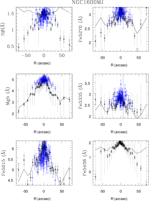
Figure 5: The lines-strength indices along the major (left) and minor axis (right). The name of the indices are labeled and the galaxies’ names are also noted. The dotted lines show the size of the systematic errors due to sky subtraction. The solid lines show the models (TMB03) predicted lines strength profiles along the axes. The blue open triangles are measurement of Sánchez-Blázquez et al. (2007).

Figure 5: Continued.

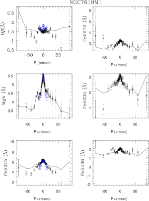
Figure 5: Continued. The blue open triangles showing the data taken from Fisher et al. (1995a).

Table 6: Format example of the measured Lick indices as a function of distance from the center (positive: east, negative: west) for the different position angles. The full table is available electronically.

Galaxy	R	PA	H$\beta\pm d$H$\beta_{stat}\pm d$H$\beta_{sys}$	Mgb	Fe5015	Fe5270	Fe5335	Fe5406
	(″)	(deg)	(Å)	(Å)	(Å)	(Å)	(Å)	(Å)
NGC1600	-69.9	9	$0.5\pm 0.1\pm 0.3$	$2.1\pm 0.1\pm 2$	$4.9\pm 0.3\pm 0.3$	$2.0\pm 0.2\pm 1.2$	$2.7\pm 0.3\pm 1.5$	$-0.4\pm 0.2\pm 3.1$

3.3 Comments on individual galaxies

NGC1600: This is the most distant galaxy of the sample and it is classified as E3. Our kinematic data extend to 70 arcsec from the center, almost about four times the radius of Bender et al. (1994). The kinematic profiles show no rotation along both axes and high velocity dispersion. The velocity dispersion shows a steep gradient inside 15 arcsec, becomes flat along the major axis and even increases along the minor axis outwards. The galaxy shows a weakly asymmetric profile of Mgb, Fe5015 and Fe5335 in the outer part. Moreover, it has low H$\beta$ line strength, particularly in the outer parts. Because accurate measurements of H$\beta$ always suffer from the contamination of emission lines or sky lines, we carefully checked the spectra, and no emission lines or sky lines were detected. Our instrumental resolution could be too low to detect the weak emission lines embed in the bandpass or some weak absorption features of other elements, such as CrI $\lambda$4885 Å, FeI $\lambda$4891 Å, set in the pseudo-continuum of H$\beta$ definition (Korn et al. 2005; Puzia et al. 2005).

NGC4125: This galaxy shows strong ionized gas emission along the major axis. The stellar kinematics were measured out to 1.7 a_e on SW side along the major axis and 3.5 b_e on NW side along the minor axis. As Fig. 3 shows, the kinematic profiles are fairly symmetric, and show a strong velocity gradient along the major axis; inside 50 arcsec the rotational velocity increases rapidly from 0 to 150 km/s, remains remains nearly flat out to 100 arcsec, and declines at larger radii.

Furthermore, it is clear from Fig. 3 that the NGC4125 shows rotation along the minor axis which could indicate triaxiality (Bertola et al. 1984), or be the sign of unsettled material left over from a past merger and visible on images of the galaxy. The velocity dispersion profile of the stars shows a depression in the inner 8 arcsec, on both the major and the minor axes. This depression suggests that there is a colder substructure in the innermost center. The galaxy presents positive gradients of H$\beta$ index both along major axis and minor axis in the center, while it remains flat towards outer part. The H$\beta$ profile along major axis exhibits weak asymmetry.

Compared to the kinematic profiles of the stars, the velocity curves of the gas along the axes shows stronger gradients, see left panel of Fig. 6, and presents a maximum of about 240km/s at 10 arcsec. Warm gas has been found already by Bertola et al. (1983). Our folded gas velocity curve is not perfectly axisymmetric, but less distorted than what reported there. Finally, the rotation curve implied by the stellar dynamical modeling is much higher ($\approx 300$ km/s) than the measured velocities. Therefore the gas is not following simple circular motions and/or is not settled in a regular disk. The gas velocity dispersion is high in the inner 20 arcsec ($\approx 160$ km/s after correction for instrumental broadening) and unconstrained at larger radii, where it is less or comparable to our spectral resolution. Figure 6 shows also the equivalent widths (in Å) of the emission line H$\beta$ and the ratios [NI]$\lambda\lambda$5197,5200/H$\beta$ and [OIII]$\lambda$5007/H$\beta$ in logarithmic units. The data along the major and minor axes are shown separately. The [NI]$\lambda\lambda$5197,5200/H$\beta$ versus [OIII]$\lambda$5007/H$\beta$ diagnostic diagram are shown at the bottom of right panel. As it can be seen from the plot, the ratios [OIII]$\lambda$5007/H$\beta$ span the range from 0 to 0.5 and the ratios [NI]$\lambda\lambda$5197,5200/H$\beta$ go from -0.5 to 0.0. According to Sarzi et al. (2010), this is the region driven by LINER-like emission.

Figure 6: The gas kinematics both along major and minor axes of NGC4125 are shown on the left; open and filled symbols show different sides of the galaxy. The emission lines (in logarithmic units) along the major and minor axes of NGC4125 are show on the right. From the first row to the third row, we show the H$\beta$ emission EW, the [OIII]$\lambda$5007/H$\beta$ and the [NI]$\lambda\lambda$5197,5200/H$\beta$ ratios (in logarithmic units) as a function of distance from the center. In the bottom panels the diagnostic plots [NI]$\lambda\lambda$5197,5200/H$\beta$ against [OIII]$\lambda$5007/H$\beta$ in logarithmic units are shown.

NGC7619: Our kinematic profiles for NGC7619 extend to almost 1.6 a_e along the major axis and 2 b_e along the minor axis, further out than previous works, for example Fisher et al. (1995a); Longhetti et al. (1998) extended only up to 2/3 R_e. Our data (circles in Fig.2) agree, within the error, with the measurement of Fisher et al. (1995a) (squares). From the kinematic profiles, we see that the velocity dispersion of the galaxy has a shallow gradient inside 10 arcsec and remains nearly flat towards large radii. The rotational velocity also remains almost constant from 8 arcsec out to 60 arcsec. Furthermore, slow rotation along the minor axis reveals that the galaxy is possibly triaxial (Bertola et al. 1984). Concerning the lines strength profiles, the galaxy shows constant H$\beta$ index from the center to the outer regions and it has a steep Mgb gradient.

4 Stellar populations

4.1 Model and method

In this section, we use the stellar population models of TMB03 to derive the age, total metallicity and element abundance gradients along the major and minor axes from the measured lines indices of our galaxies. The TMB03 models cover ages between 1 and 15 Gyr, metallicities between 1/200 and 3.5 solar. Furthermore, the models take into account the effects on the Lick indices by the variation of element abundance, hence, give Lick indices of simple stellar populations not only as the function of age and metallicity, but also as the function of the $\alpha/Fe$ ratio. The age, total metallicity and element abundance can be derived from a comparison of selected line strength indices with SSP models TMB03.

The traditional and effective method of studying stellar population properties uses diagrams of different pairs of Lick indices (Thomas et al. 2005a). The $H\beta$ versus [MgFe]´ pair diagram is selected as the best age indicator because $H\beta$ is sensitive to warm turnoff stars and [MgFe]´ index is considered as the best detector of metallicity since it does not depend on abundance ratio variations. Using $H\beta$ versus [MgFe]´ can break the age-metallicity degeneracy. The $<Fe>=(Fe5270+Fe5335)/2$ versus Mgb pair usually is considered as the best indicator of the abundance of populations. However, in this study, following Saglia et al. (2010) we use a simple and perhaps more accurate method- $\chi^{2}$ minimization:

$$\chi^{2}=\sum_{index[i]}\frac{(index_{i[ob]}-index_{i[mod]})^{2}}{(\sigma_{i[ob]})^{2}}$$ (3)

where $index_{i[ob]}$ and $index_{i[mod]}$ represent the $i^{th}$ observational indices and model indices respectively, $\sigma_{i[ob]}$ is the observational uncertainty of $i^{th}$ indices. The best fitting age, metallicity and $\alpha/Fe$ can be derived by finding the minimum $\chi^{2}$ of all selected lines indices to the SSP models. We chose H$\beta$, Mgb, $Fe_{5015}$, $Fe_{5270}$, $Fe_{5335}$ and $Fe_{5406}$ as the indicators. Further, in order to improve the precision of the stellar properties using the $\chi^{2}$ minimization method we interpolated the tabulated indices of TMB03 on steps of 0.1 Gyr in age, 0.02 in metallicity and 0.05 in $\alpha/Fe$.

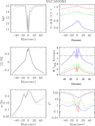
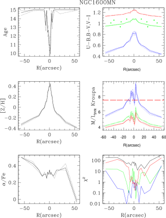
Figure 7: The best fitting SSP equivalent age, metallicity and element abundance ratio are showed in the left in each plot. The right top of each plot shows the Johnson broad band U-B, B-V, V-I colors profiles, the blue and red solid lines stand for U-B and B-V color respectively; the black solid lines indicate the V-I color. For NGC4125 and NGC7619 the measured V-I color of Bender et al. (1989) are shown as dots. In the case of NGC1600, the aperture B-V color taken from (Sandage 1973) are indicated. The M/L_BVI are shown in the mid of the right columns, the blue, green and red solid lines indicate the M/L in the B, V and I band respectively; the red dashed line shows the best-fit dynamical M/L in the I band for NGC4125 and NGC7619 and in the R band for NGC1600; the minimized $\chi^{2}$ of selected line strengths are presented in the bottom panel on the right, red, blue and green lines present the minimized $\chi^{2}$ of H$\beta$, Mgb and Fe₅₀₁₅ respectively; while the black lines show the total minimized $\chi^{2}$.

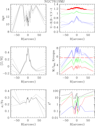
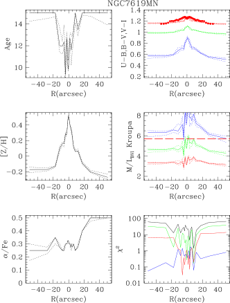
Figure 7: Continued.

4.2 Ages, metallicities and $\alpha/Fe$ ratio profiles

The model predicted lines strength profiles are shown in Fig. 5 with solid lines. The derived quantities (age, metallicity, element abundance, colors, mass-to-light ratios, and resulting $\chi^{2}$) are shown in Fig. 7. Here we average together every four points to reduce the scatter. The theoretical lines strength indices match well the measured parameters in the inner regions of the galaxies, although an acceptable value of $\chi^{2}\approx 3$ is obtained seldom (see Fig. 7), possibly indicating a global underestimation of our statistical errors, or, more probably, the presence of systematic effects. In particular, in the case of NGC1600, the large values of $\chi^{2}$ are mainly driven by the significantly low H$\beta$ (Fig. 5 and red solid lines in the right bottom panel of Fig. 7). The large values of $\chi^{2}$ in the outer regions along the minor axis of NGC4125 are caused by the lower H$\beta$ strength. In the case of NGC7619, the large values of $\chi^{2}$ in the outer parts along both the major and the minor axes are mainly due to large divergence of Fe5015 (green solid lines). The SSP equivalent age, metallicity and element abundance ratio along the major and minor axis of our galaxies are also plotted on the left side of each panel. In each panel the solid lines indicate the fitting parameter profiles and the dotted lines show the 1 $\sigma$ errors. As it can be seen in Fig. 7, all the galaxies are $[\alpha/Fe]$ overabundant, at the value of 0.25, 0.1 and 0.3 dex for NGC1600, NGC4125 and NGC7619 respectively. The $\alpha/Fe$ ratios are fairly constant in the central regions, with hints for a decrease in the outer parts. Table 7 lists the slope of $\triangle\mbox{index}/\triangle log(r)$ of our galaxies which were derived by fitting a straight line to our measured data points.

Table 7: Line strength and total metallicity gradients:$\triangle$ index/ $\triangle$ log (r).

Galaxy	Range	Mgb	Fe5015	Fe5270	Fe5335	$<Fe>$	Fe5406	H$\beta$	Z/H	$\alpha/Fe$	Age
Name	($R_{e}$)	Slope	Slope	Slope	Slope	Slope	Slope	Slope	Slope	Slope	Slope
		$\pm$	$\pm$	$\pm$	$\pm$	$\pm$	$\pm$	$\pm$	$\pm$	$\pm$	$\pm$
NGC1600	0-0.5	-0.787	-0.339	-0.179	-0.196	-0.187	-0.207	-0.125	-0.342	-0.042	1.32
		0.067	0.082	0.036	0.053	0.038	0.094	0.028	0.029	0.012	0.43
	0-1	-0.742	-0.537	-0.268	-0.222	-0.245	-0.236	-0.172	-0.288	-0.044	1.398
		0.069	0.085	0.037	0.046	0.036	0.029	0.033	0.028	0.009	0.343
NGC4125	0-0.5	-0.378	-0.328	-0.215	-0.267	-0.241	-0.121	0.224	-0.225	-0.037	-3.527
		0.021	0.036	0.038	0.020	0.024	0.017	0.020	0.013	0.006	1.234
	0-1	-0.464	-0.405	-0.260	-0.319	-0.289	-0.185	0.173	-0.235	0.008	-2.464
		0.023	0.035	0.033	0.020	0.021	0.019	0.020	0.014	0.006	1.250
NGC7619	0-0.5	-0.711	-0.571	-0.192	-0.352	-0.272	-0.299	0.078	-0.343	0.041	-1.420
		0.049	0.082	0.035	0.038	0.028	0.036	0.021	0.028	0.010	0.614
	0-1	-0.787	-0.953	-0.280	-0.437	-0.359	-0.264	-0.026	-0.327	-0.034	2.143
		0.048	0.103	0.035	0.037	0.028	0.036	0.039	0.024	0.011	0.497

The nuclear (inside R_e/8) parameters were derived by Trager et al. (2000b) and Denicoló et al. (2005). In order to compare to values available in the literature we calculate the mean parameters inside R_e/8. For NGC1600 and NGC7619 Trager et al. (2000b) derived the nuclear parameters [age, Z/H, $\alpha/Fe$] with [8.6 $\pm$ 1.7 Gyr, 0.35 $\pm$ 0.05, 0.22 $\pm$ 0.02] and [14.8 $\pm$2.3 Gyr, 0.2 $\pm$ 0.03, 0.18 $\pm$ 0.01] which compare to our value of [ 13.1 Gyr $\pm$ 1.1, 0.35 $\pm$ 0.03, 0.317 $\pm$ 0.001] and [ 11.7 Gyr $\pm$ 0.9, 0.25 $\pm$ 0.02, 0.284 $\pm$ 0.001] respectively. In the case of NGC4125, Denicoló et al. (2005) obtained [age, Z/H, $\alpha/Fe$] with [5.9 $\pm$3 Gyr, 0.32 $\pm$ 0.1, 0.1] while we find [ 10.1 Gyr $\pm$ 0.6, 0.12 $\pm$ 0.02, 0.095 $\pm$ 0.001].

4.3 Color and M/L profiles

The Johnson broad band U-B, U-V, B-V, V-R, V-I, V-K, J-K, J-H, H-K color and M/L ratio in B, V, R, I, J, H, and K bands profiles were calculated using the Kroupa initial mass function Kroupa (1995) with the help of the SSP models (Maraston 1998). For a clear presentation in the figures, we only show the U-B, B-V and V-I color and the mass to light ratios in B, V, I band in this papers. On the top right panels in Fig. 7, the blue and red solid lines stand for U-B and B-V color respectively; the black lines indicate the V-I color. For NGC4125 and NGC7619, the measured V-I color are also over plotted with solid dots. For NGC1600, unfortunately, we do not have reliable broad band color profiles and we take the aperture B-V color from Sandage (1973). As it can be seen from the plots, the models predicted color profiles agree reasonably well with the measured colors except for small discrepancies. We note that Maraston et al. (2009) discuss the limitations of current SSP models in predicting accurate colors. In particular, the B-V colors of old ($\sim 12$ Gyr), solar metallicity SSP models are expected to be -0.09 mag bluer than what used here, while the differences are smaller for the redder colors. In addition, if our estimated ages are too small because of the presence of a second younger component (Serra & Trager 2007), then the predicted SSP colors would be biased and bluer than they should. Moreover, SSP models do not account for the presence of dust, which could be present especially at the centers of our galaxies. The middle right of Fig.7 shows the theoretical M/L ratio in B, V, I bands; the blue and green lines display the M/L ratios in B and V bands respectively; while the red lines present the I band M/L ratios. The red long dashed lines show the dynamical M/L in the I band for NGC4125 and NGC7619, and in the R band for NGC1600 (see Sect. 5). The minimized $\chi^{2}$ of selected lines strength are presented in the bottom panel on right, red, blue and green lines present the minimize $\chi^{2}$ of H$\beta$, Mgb and Fe₅₀₁₅ respectively; while the black lines show the total minimized $\chi^{2}$. All of the our giant elliptical galaxies show a red sharp peak, mainly due to metallicity gradients (Peletier 1989).

5 Line strengths and the local escape velocity

As discussed in the Introduction, we want to exploit the link that the galaxy formation process has established between the Mgb line strength and the local escape velocity to constrain the density profile of dark matter halos in the outer regions of galaxies. The $V_{esc}$ is given by:

$$V_{esc}=\sqrt{2|\Phi|},$$ (4)

and therefore at each radius it is sensitive to the total mass density profile up to very large radii; for example, in the case of a spherical density distribution $\rho$ the gravitational potential $\Phi$ is:

$$\Phi(r)=-G\left[\frac{M(<r)}{r}+4\pi\,\int_{r}^{\infty}\rho(r^{\prime})r^{\prime}dr^{\prime}\right],$$ (5)

where $M(<r)=4\pi\int_{0}^{r}r^{\prime 2}\rho(r^{\prime})dr^{\prime}$. In the following we will correlate Mgb measured at the projected distance $r$ with $V_{esc}$ computed at the intrinsic distance $r$. As noted by Scott et al. (2009), we see no difference if instead we compute the projected quantity:

$$V_{esc,pr}=\frac{\int V_{esc}\,\rho_{\ast}\mathrm{d}z}{\int\rho_{\ast}\,\mathrm{d}z}$$ (6)

where $z$ is the line-of-sight. Moreover, having in mind the physical scenario described in the Introduction, where more enrichment in Mgb is achieved if more gas is retained, one would expect the difference $\Delta V$ between $V_{esc}(r)$ and the average velocity of stars and gas at that location $r$ to play the crucial role. In fact, $\Delta V$ happens to be proportional to $V_{esc}$, because elliptical galaxies are virialized systems.

5.1 Dynamical models

We use the axisymmetric Schwarzschild’s orbits superposition technique (Schwarzschild 1979) to derive the gravitational potential profiles. Thereby, also the stellar mass-to-light ratio, the internal orbital structure as well as the velocity anisotropy of the galaxies can be determined. Here, we only briefly present the basic steps, details about our implementation of the method are given in Thomas et al. (2004, 2005b).
(1): We first determine the luminosity density from the surface brightness profile. The photometric data for the modelling are deprojected into a three-dimensional, axisymmetric distribution with specified inclination using the program of Magorrian (1999).
(2): The total mass distribution of the galaxies consists of the stellar mass density and a dark matter halo:

$$\rho={\Upsilon}{\nu}+\rho_{DM},$$ (7)

where $\Upsilon$ is the stellar mass-to-light ratio, and ${\nu}$ is the deprojected stellar luminosity density.
(3): The gravitational potential $\Phi$ can be derived by integrating Poisson’s equation once the total mass profile is obtained. Thousands of orbits are calculated in this fixed potential.
(4): The orbits are superposed to fit the observed LOSVDs, following the luminosity density constraint. The maximum entropy technique of Richstone & Tremaine (1988) is used to fit the kinematics data by maximizing the function:

$$$\^{S}$=S-{\alpha}\chi_{kin}^{2},$$ (8)

where S is an approximation to the Boltzmann entropy and ${\chi}^{2}$ is the sum of the squared residuals to the kinematic data. The smoothing parameter ${\alpha}$ controls the influence of the entropy S on the orbital weights, see Thomas et al. (2004) for more details.

Two different types of dark matter halo distribution were tried to recover the mass profiles. First, the NFW halo profile (Navarro et al. 1996):

$$\rho_{NFW}(r)=\frac{\rho_{s}}{(r/r_{s})(1+r/r_{s})^{2}},$$ (9)

where $\rho_{s}$ is the characteristic density of the halo and $r_{s}$ is a characteristic radius. One further defines the so-called concentration parameter $c$ of the halo that is related to $r_{s}$ and the viral radius $r_{200}$ via $r_{s}=r_{200}/c$. The potential generated by this density distribution is given by:

$$\Phi(r)=4{\pi}G\rho_{s}{r_{s}}^{2}\frac{r_{s}}{r}\ln(r+\frac{r}{r_{s}}),$$ (10)

where G is the gravitational constant. The second halo used is the cored logarithmic (LOG) halo profile (Binney & Tremaine 1987) , that reads as:

$$\rho_{LOG}(r)=\frac{{V_{c}}^{2}}{4{\pi}G}\frac{3{r_{c}}^{2}+r^{2}}{({r_{c}}^{2}+r^{2})^{2}}.$$ (11)

This gives a roughly constant circular velocity $V_{c}$ and a flat density core inside $r<r_{c}$. The potential is given by:

$$\Phi(r)=\frac{V_{C}^{2}}{2}\ln(r^{2}+r_{c}^{2})$$ (12)

Both the NFW and the LOG potential give divergent mass profiles when integrated to infinity. In our numerical implementation the potential is computed up to 10 effective radii and extrapolated Keplerian at larger radii. In order to investigate further the physical extent of such halos we introduce a cut-off radius $r_{cut}$ and modify the density profile given by Eq. 11 as follows:

$$\rho_{cut}(r)=\rho_{LOG}(r)\times\exp\left(-\frac{r^{2}}{r_{cut}^{2}}\right).$$ (13)

5.2 Model results for NGC1600, NGC4125 and NGC7619

Photometric data: We produced isophotal fits separately on the HST and the ground based images using the code of Bender & Möllenhoff (1987). For NGC4125 and NGC7619, the surface brightness profiles consist of HST F814W(I) filter images and SDSS $i$ band images, scaled to I band. The photometric data of NGC4125 extended to 216 arcsec, about 3.5 times of effective radius. For NGC7619, the photometric data extended to 167 arcsec, more than 5 times of its effective radius. In the case of NGC1600, the photometric data came from HST images observed with the F555W(R) filter and scaled to the profile of Peletier et al. (1990). They extend to 200 arcsec, nearly 4.5 times of the effective radius. The photometric data are deprojected into the 3d luminosity distribution using the program of Magorrian (1999). Kinematic data set: The kinematics data both along the major axes and minor axes derived in Sect. 3.1 are used.

We tested models at three different inclinations (i = 70, 80, 90) for our galaxies, the best-fit models for all three galaxies are edge-on ($i=90$). The dark halo parameters for the best-fit logarithmic halos are given in Tab. 8. They fit very well to the dark matter determinations of Coma early-type galaxies by Thomas et al. (2009). We also tested dark matter halos following the NFW halo profile, as in Thomas et al. (2005b). The best-fit NFW-halos for NGC1600, NGC4125 and NGC7619 require concentration parameters c = 5, 5.5, 7.5 respectively. The mass-to-light ratios derived with NFW profile are similar to the mass-to-light ratios with logarithmic halo profile. Fig. 7 shows that the mass-to-light ratios derived from the SSP models with a Kroupa IMF are on average 45% lower than the dynamical ones, similarly to Cappellari et al. (2006). A better agreement is achieved if a Salpeter IMF is considered. The comparison with the mass profiles derived from X-ray measurements for NGC4125 and NGC7619 (Fukazawa et al. 2006) is good: our total masses within the last kinematic point are just 10% larger than the X-ray ones. For NGC1600 the discrepancy is larger, with X-ray masses underestimating the stellar kinematics ones by 30 (NFW potential) or 40 % (LOG potential).

As a further step, we compute a number of models with varying $r_{cut}$ from 5 to 10 times effective radii for each galaxy. The different cut-off radii of the dark matter halos do not have significant effects on the dynamical parameters ($\Upsilon$, $V_{c}$, $r_{c}$), nor the quality of the kinematic fit (see upper panel of Fig. 8, where the self-consistent model without dark matter is plotted at $r_{cut}=0$ and the model with no cutoff at $r_{cut}=80$ kpc), as soon as models with $r_{cut}\geq 40$ kpc are considered. However, they do have an effect, when we also take into account the correlation $Mg_{b}-V_{esc}$.

Table 8: Halo circular velocity $V_{c}$, halo core radius $r_{c}$, average dark matter density $<\rho_{\mathrm{DM}}>$ (within $2\,r_{\mathrm{eff}}$) and stellar mass-to-light ratio $\Upsilon$ (last column: photometric band) for the best-fit dynamical models of NGC1600, NGC4125 and NGC7619 (no cutoff radius).

Name	$V_{c}$	$r_{c}$	$\log_{10}<\rho_{\mathrm{DM}}>$	$\Upsilon$	band
	(km/s)	(kpc)	($M_{\odot}/pc^{3}$)	($M_{\odot}/L_{\odot}$)
NGC1600	$350^{+250}_{-50}$	$31^{+62}_{-12}$	$-2.1\pm 0.5$	$7.3\pm 0.5$	R
NGC4125	$350^{+100}_{-100}$	$32^{+7}_{-7}$	$-2.2\pm 0.1$	$5.7\pm 0.7$	I
NGC7619	$600^{+200}_{-150}$	$49^{+9}_{-16}$	$-2.0\pm 0.2$	$6.5\pm 0.5$	I

5.3 Mgb, the local escape velocity and the size of dark matter halos

Next we explore the correlation between Mgb and the local escape velocity by fitting log Mgb and log $V_{esc}$ to a straight-line, weighted by the errors. We computed errors on $V_{esc}$ by considering at every point the range of escape velocities allowed by all models giving $\chi^{2}_{kin}\leq\chi^{2}_{kin,min}+1$. According to eq. (5) the outer halo-profile has a considerable effect on $V_{esc}$ and, hence, on the tightness of the correlation between log Mgb and log $V_{esc}$. Here, we explore shallower halo profiles than probed by Scott et al. (2009) and use the correlation between Mgb and $V_{esc}$ to constrain the size of dark matter halos. We define a new parameter ${{\chi}_{tot}}^{2}$, given by:

$$\chi_{tot}^{2}=\chi_{Mgb}^{2}+\chi_{kin}^{2},$$ (14)

where, $\chi_{Mgb}^{2}$ quantifies the goodness of fitting log Mgb and log $V_{esc}$ to a straight-line. The $\chi_{kin}^{2}$ is mentioned above, it quantifies the deviation between model and observed kinematics.

We probed two different radial scalings: (1) correlating the measured Mgb(r) at radius $r$ with the escape velocity $V_{esc}(r)$ at the same radius $r$ and (2) correlating Mgb with the escape velocity on the corresponding isophote (i.e. we compare the Mgb measured at a distance $b$ from the galaxy centre along the minor-axis with $V_{esc}(b/\sqrt{q})$ in the equatorial plane and the Mgb measured at a distance $a$ from the galaxy centre along the major-axis with $V_{esc}(a\sqrt{q})$, where $q=1-\epsilon$ is the apparent flattening of the light-distribution). Scaling (2) gives a smaller $\chi_{tot}^{2}$ and is discussed in the following. Using the scaling (1), however, gives similar results with respect to the halo core radii.

The lower panel in Fig. 8 shows $\chi_{tot}^{2}$ as a function of the cut-off radius in kpc. The minimum scatter is achieved for $r_{cut}=60$ kpc. This is 4.3 times the effective radii for NGC1600, 9.5 times for NGC4125 and 8.5 times for NGC7619. Lower cutoff radii give slightly worse $Mgb-V_{esc}$ correlations, but the trend is significant only in combination with $\chi^{2}_{kin}$. Cutoff radii larger than 70 kpc have significantly higher $\chi^{2}_{tot}$. As discussed above, this is driven only by the $Mgb-V_{esc}$ correlation.

The Mgb-$V_{esc}$ correlation with the lowest $\chi^{2}_{tot}$ is

$$\log\mathrm{Mg}b=(0.873\pm 0.008)\times\log\,V_{esc}-(2.105\pm 0.024)$$ (15)

(shown in the bottom part of Fig. 9 by the solid line), the corresponding $\chi_{Mgb}^{2}$ is 592 (for 368 data points). The correlation for the best-fitting NFW halo reads

$$\log\mathrm{Mg}b=(0.629\pm 0.004)\times\log\,V_{esc}-(1.314\pm 0.013)$$ (16)

(shown by the long dashed-dotted line), the corresponding $\chi_{Mgb}^{2}$ is 1360. The regression obtained for models without dark matter is shifted to lower $V_{esc}$, but is steeper than reported by Scott et al. (2009). For comparison, in the upper plot of Fig. 9 we show the Mgb-$V_{esc}$ relation obtained when the best-fitting logarithmic halo models without cutoff are used. Note that we get the same cut-off radii if we use $[Z/H]-V_{esc}$ instead of Mgb-$V_{esc}$.

Figure 8: The $\chi_{kin}^{2}$ as a function of cut-off radius summed over all three galaxies is shown in the upper panel and the $\chi_{Mgb}^{2}$ is presented in bottom panel. The dotted lines shows the $\chi^{2}$ for the NFW halo profile, and the last point is the $\chi^{2}$ for the LOG dark halo profile without cutoff.

Figure 9 indicates that the simple linear relation between $\log V_{esc}$ and $\log Mgb$ breaks down in the outer regions of the galaxies investigated here. There, the measured value of $Mgb$ is much smaller than the linear relation determined in the inner parts of the galaxies would predict. Due to the relatively low number of points involved, the bending of the relation does not influence the result of Fig. 8: the same optimal cut-off radius is found if we do not consider points with $\log Mgb<0.5$. However, this might be telling something about the formation process of ellipticals. It is reminiscent of several recent observational and theoretical findings (van Dokkum et al. 2010, and references therein) that suggest that the outer stellar envelopes of bright ellipticals might be the result of later accretion of smaller objects on older central cores formed in violent collapsing processes at high redshift. In this case, the metallicity measured in the outer parts would be set be the (lower) escape velocity of the accreted objects, and not by the deeper potential well of the final giant elliptical.

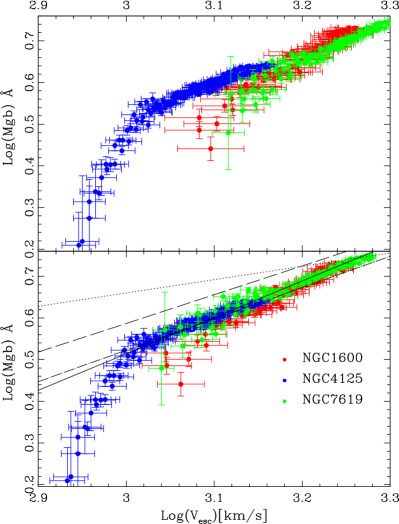
Figure 9: The upper panel and bottom panel show the correlation between log(Mgb) and log($V_{esc}$) derived using LOG dark matter halos without cut off and cut off at 60 kpc respectively. Different colour refer to different galaxies. The full line is the corresponding best fit. The dashed-dotted lines is computed for NFW dark matter halos. The long-dashed line shows the regression obtained when models without dark matter halo are considered. The dotted line is taken from Scott et al. (2009) without dark matter halos.

Figure 10 shows the total density profile derived for NGC1600 for the different cases discussed above (self-consistent, with a logarithmic dark matter halo with or without cut-off, or with a NFW halo). Clearly, the $V_{esc}-Mgb$ correlation allows us to constrain the outer shape of the total matter density, rather than delivering a precise determination of the radius where the dark matter halos terminate. In the next section we discuss this degeneracy in more detail.

Figure 10: The total density profile derived for NGC1600 for the self-consistent model (dot-dashed line), the LOG dark matter halo cut at 60 kpc (full line), the LOG dark matter halo without cutoff (dotted line), and the NFW dark matter halo (dashed line).

5.4 The degeneracy between outer halo slope and cut-off radius

A steeper outer halo slope results in less mass in the outer regions and, thus, a lower escape velocity. Likewise, a lower cut-off radius reduces the outer mass and the escape velocity as well. Consequently, a steeper density fall-off in the outer halo region could be partly compensated for by a larger cut-off radius. In the following we investigate this degeneracy quantitatively with spherical test models.

The test models are set up as follows. We assume that the galaxy’s light distribution can be described by a Hernquist sphere (Hernquist 1990). For simplicity we assume that the mass-to-light ratio equals one in appropriate units. Then, the stellar mass distribution $\rho_{\ast}$ reads

$$\rho_{\ast}=\frac{M}{2\pi}\frac{a}{r}\frac{1}{r(r+a)^{3}},$$ (17)

where $M$ is the total stellar mass and $a$ is the scaling radius (Hernquist 1990). In the following we use $M=3\times 10^{11}\,M_{\odot}$ and $r_{\mathrm{eff}}=10$ kpc ($r_{\mathrm{eff}}\approx 1.8a$ for the Hernquist sphere). To investigate the degeneracy between slope and cut-off radius we seek a halo-profile whose slope can be adjusted conveniently. For example

$$\rho_{\mathrm{DM}}=\frac{\rho_{0}}{(r+r_{0})^{\gamma}}\times\exp\left(-\frac{r^{2}}{r_{\mathrm{cut}}^{2}}\right).$$ (18)

The four free parameters here are the normalisation $\rho_{0}$, a scaling radius $r_{0}$ (inside which the halo density eventually becomes constant), the cut-off radius $r_{\mathrm{cut}}$ and the asymptotic logarithmic slope $\gamma$ (in the absence of a cut-off). For the rest of this section we fix two of these parameters according to empirical scaling relations for early-type galaxies. Firstly, the normalisation $\rho_{0}$ is chosen such that

$$\rho_{\ast}(1.5\,r_{\mathrm{eff}})=\rho_{\mathrm{DM}}(1.5\,r_{\mathrm{eff}})$$ (19)

(Thomas et al. 2007b). Secondly, the halo scaling radius is fixed to $r_{0}=2.5\,r_{\mathrm{eff}}$ (Thomas et al. 2009).

Since the goal is to investigate how much the outer slope is degenerate with the cut-off radius we first construct an input escape-velocity profile by fixing the remaining halo parameters $\gamma$ and $r_{\mathrm{cut}}$ to some values, e.g. $\gamma=2$ and $r_{\mathrm{cut}}=5\,r_{\mathrm{eff}}$. We calculate the corresponding escape velocity profile $V_{esc}$ from the total potential

$$\Phi=\Phi_{\ast}+\Phi_{\mathrm{DM}},$$ (20)

where $\Phi_{\ast}$ is given analytically for the Hernquist sphere (Hernquist 1990) and $\Phi_{\mathrm{DM}}$ is obtained by numerically integrating equation (5) for $\rho_{\mathrm{DM}}$ of equation (18). We project the escape velocity via Eq. 6. Note that the projection does not affect the results discussed below. For the aim to study the degeneracy between halo slope and cut-off radius we assume that the projected escape velocity is given at 20 logarithmically spaced radii between $0.1\,r_{\mathrm{eff}}$ and $5\,r_{\mathrm{eff}}$, with an uncertainty of $\Delta\log V_{esc,pr}=0.05$ (see Fig.9).

Can we fit the so constructed escape-velocity profile also if we make a wrong assumption upon the halo slope? To answer this question, the slope is reset, e.g. $\gamma=3$ and the remaining free parameter $r_{\mathrm{cut}}$ is fitted such that the $\chi^{2}$ between the input escape-velocity profile and the corresponding profile with the new halo-slope is minimised. Fig. 11 shows that for a wide range of outer halo-slopes – we probed $\gamma\in[2,3.6]$ – the escape-velocity profile can be reproduced well (with a $\chi^{2}<1$). As expected, a steeper halo-slope requires a larger cut-off radius to compensate for the lowered outer mass-density. Our first result is therefore that with the given uncertainties on the escape-velocity there is a large uncertainty in the outer halo-slope and cut-off radius, related to the degeneracy between the two.

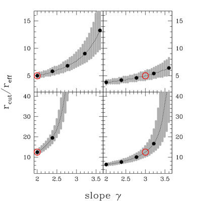
Figure 11: Fitted cut-off radius $r_{\mathrm{cut}}$ against halo-slope. The input model is indicated by the red open circle. The filled black dots show the best-fit cut-off radius for halo-slopes $\gamma=2,2.4,2.8,3.2,3.6$. Small grey dots indicate the region within $\Delta\chi^{2}\leq 1$ with respect to the input model. Left panels: input-slope $\gamma=2$ (isothermal-like); right panels: input-slope $\gamma=3$ (NFW-like). Top row: input $r_{\mathrm{cut}}=5\,r_{\mathrm{eff}}$; bottom row: input $r_{\mathrm{cut}}=12.5\,r_{\mathrm{eff}}$.

In our standard modeling, the halo-slope is $\gamma\approx 2$ (cf. Eq. 11). Next we ask how much this assumption can bias the ’measured’ cut-off radii if the actual halo-slope is steeper. To this extent we repeated the above analysis for a wide range of input cut-off radii ($r_{\mathrm{cut}}/r_{\mathrm{eff}}\in[5,20]$) and an input slope of $\gamma=3$. The choice of $\gamma=3$ is driven by the fact that pure dark matter cosmological $N$-body simulations predict a halo profile close to Eq. (9), i.e. $\gamma=3$. For each input model, we determined the 68% confidence region that would result under the assumption of $\gamma=2$. Fig. 12 shows that cut-off radii reconstructed with $\gamma=2$ are always too small – as already discussed above. The figure also shows that if the true cut-off radius is increased by a factor of four, the reconstructed one (with $\gamma=2$) increases only by factor of two. In other words, if the steepness of the halo density profile is underestimated then (1) the cut-off radii are biased too low and (2) a relatively small uncertainty in the ’measured’ $r_{\mathrm{cut}}$ – obtained under the assumption of a $\gamma=2$ – may correspond to a relatively large uncertainty in the true cut-off radii if the real value of $\gamma$ is significantly larger than two.

Figure 12: Reconstructed halo cut-off radii (assuming an outer halo-slope $\gamma=2$) against true cut-off radii (the true halo-slope is $\gamma=3$). The points show the 68% confidence region of the reconstructed cut-off radii. The dotted line is the one-to-one relation. An underestimation of the steepness of the halo density profile results in an underestimation of the cut-off radius.

6 Discussion and summary

Accurate kinematic profiles extending out to 1.5 to 2 $R_{e}$ along the major and minor axis for the three giant elliptical galaxies NGC1600, NGC4125 and NGC7169 have been measured, together with 6 lines strength Lick indices. For NGC4125 we also detected gas emission along the major axis and measured its kinematics and equivalent width strength. From the comparison of the [NI]$\lambda\lambda$5197,5200/H$\beta$ vs [OIII]$\lambda$5007/H$\beta$ diagnostic diagram to the previous work, we concluded that the emission region is probably caused by LINER-like emission.

With the help of the SSP models, we derived the stellar population parameters, the M/L ratios and the broad band colors of our galaxies. We found the galaxies NGC1600 and NGC7619 have high metallicities, in contrast, the galaxy NGC4125 is just slightly above solar metallicity. The three objects have significant metallicity gradients. All of the galaxies are overabundant, NGC4125 just by $0.1$ dex, and do not have significant gradients of element abundances along the axes. These galaxies have sharp red peaks at the center, reflecting the steep change of metallicity and in agreement with the models predicted color profiles.

According to the simple element enrichment scenario, the $\alpha$ elements are mainly delivered by Type II supernovae explosions of massive progenitor stars, and a substantial fraction of Fe peak elements come from the delayed exploding Type Ia supernovae (Nomoto et al. 1984; Thielemann et al. 1996). Thus the $\alpha/Fe$ can be used as an indicator to constrain the formation timescale of stars. Hence the absence of radial variations of $\alpha$/Fe ratio in our galaxies likely suggests that there is no radial variation of star formation time scales. The radial metallicity and lines strength gradients give one of the most stringent constraints on the galaxy formation. The galaxies that form monolithically have steeper gradients and the galaxies that undergo major mergers have shallower gradients. The mean metallicity gradients for non-merger and merger galaxies derived by theoretical simulation in Kobayashi (2004) are $\triangle$[Z/H]/$\triangle$ log(r) $\sim-0.30\pm 0.2$ and $-0.22\pm 0.2$, respectively. The author found that the galaxies with gradients steeper than -0.35 are all non-major merger galaxies. As it can be seen from Table 7 the gradients $\triangle[Z/H]/\triangle\log(r)$ of our galaxies are compatible with numerical simulations. At face value, there is a weak indication that NGC1600 and NGC7619 were formed through a monolithic collapse process, while NGC4125 was shaped via a (recent) major merger as also indicated by minor-axis rotation, the presence of gas, young central stellar ages, just mild $\alpha$/Fe-overabundance and the unrelaxed appearance of the outer stellar envelope.

Using the axisymmetric Schwarzschild’s orbits superposition technique (Schwarzschild 1979) with and without dark halos, we derived the local escape velocity of these galaxies. From the correlation between Mgb, and the local escape velocity, we further confirmed the suggestion of Franx & Illingworth (1990) that metallicity and lines strength are a function of local escape velocity. Moreover, we considered models with logarithmic dark matter halos of different sizes. The best fitting Mgb-$V_{esc}$ relation comes from models which cut off the logarithmic halo at 60 kpc. Similar cut-off radii are obtained when using the correlation between $[Z/H]$ and $V_{esc}$, but the scatter in this relation is larger, because it also depends on the stellar population age (see also Scott et al. 2009). We find that – at a given escape velocity – the youngest of our galaxies, NGC4125, is also the most metal-rich one, which could be explained within a merger scenario as star formation from enriched material.

Our cut-off radii agree with the lensing analysis of cluster galaxies by Halkola et al. (2007) but not with the results from X-rays and strong-lensing (Humphrey & Buote 2010; Koopmans et al. 2009). Larger cut-off radii are compatible with the data if dark matter halos with steeper outer density profiles are considered.

We discover deviations from a linear correlation between log Mgb and log $V_{esc}$ in the outer parts of our galaxies, where the measured Mgb are lower than predicted by the extrapolation from the correlation further inside. The physical link between $V_{esc}$ and Mgb is established at the main time of star formation activity of the galaxy. Dry mergers happening after this episode will increase $V_{esc}$ without increasing Mgb. Hydrodynamical cosmological simulations by Naab et al. (2009) indicate that the outer parts of massive ellipticals (beyond $\ga 5\,\mathrm{kpc}$) might be dominated by stars which were born in low-mass halos and accreted by frequent minor mergers. If this would be the dominant process for the formation of the outer parts of giant ellipticals one would expect such a break-down of the linear correlation between log Mgb and log $V_{esc}$ as observed, because the outer Mgb would come from stars which were formed in small halos with low $V_{esc}$ (and accordingly low Mgb).

We plan to further investigate the connection between line strengths and dark matter halos with a more extended galaxy sample.