Edge Dynamics in a Quantum Spin Hall State:
Effects from Rashba Spin-Orbit Interaction

Abstract

We analyze the dynamics of the helical edge modes of a quantum spin Hall state in the presence of a spatially nonuniform Rashba spin-orbit (SO) interaction. A randomly fluctuating Rashba SO coupling is found to open a scattering channel which causes localization of the edge modes for a weakly screened electron-electron (e-e) interaction. A periodic modulation of the SO coupling, with a wave number commensurate with the Fermi momentum, makes the edge insulating already at intermediate strengths of the e-e interaction. We discuss implications for experiments on edge state transport in a HgTe quantum well.

The quantum spin Hall (QSH) state is a recently discovered phase of electronic matter in two dimensions which exhibits no symmetry breaking KaneMele ; Bernevig . Being an example of a topological insulator HasanKane , the QSH state is gapped in the bulk but exhibits massless edge modes. These modes propagate in opposite directions for opposite spins, each helical mode having a time-reversed copy. In the range of electron-electron (e-e) interactions probed in experiments Konig , elastic backscattering induced by a single (nonmagnetic) impurity or by quenched disorder is suppressed by time-reversal invariance Wu ; Xu . For samples of a length smaller than the spin dephasing length Jiang one thus expects that the edge modes are protected, resulting in nondissipative transport with a quantized Landauer conductance $2e^{2}/h$. This expectation is supported by experiments Konig , holding promise for exploiting QSH edges in future integrated circuit technology as a means to reduce power dissipation as devices become smaller.

The question whether the QSH edge is stable also against e-e interactions in the presence of a Rashba spin-orbit (SO) interaction has received less attention. One should here recall that SO interactions $-$ which allow for spin-flip scattering while respecting time-reversal invariance $-$ come in different guises. In the case of a HgTe quantum well $-$ the best studied platform for realizing a QSH state Konig ; BHZ $-$ the intrinsic SO interaction in the atomic $p$ orbitals crucially contributes to the very special properties of this material: For a quantum well (QW) thicker than a critical value it inverts the band structure, pushing the $p$ band above the $s$ band. A simple model calculation reveals the presence of a single pair of helical edge bands inside the inverted bulk band gap, showing that this intrinsic SO interaction is what makes possible the QSH state Konig2 . This is to be contrasted with the Rashba SO interaction which originates from the gate-controllable inversion asymmetry of a QW Winkler . Its strength can be huge in the bulk metallic phase of an inverted HgTe structure, with an effective coupling several times larger than for most other known semiconductor heterostructures Gui . In a QSH state with an insulating bulk, charge and spin are transported by the edge modes. With the bands for these modes dispersing all the way from the bulk valence band to the bulk conduction band Konig2 , one expects a sizable Rashba interaction to still operate at the edge of the sample, making it important to inquire about its effect on the edge modes.

In this Letter we analyze the dynamics at the QSH edge in the presence of a Rashba SO interaction. Treating the Rashba interaction as a perturbation, we find that it has no effect on the propagation of edge modes when it is spatially uniform. The more realistic case when the Rashba coupling fluctuates randomly in space Sherman ; Golub is different, however. Together with a weakly screened e-e interaction, the Rashba interaction now opens a scattering channel for the edge modes which may cause them to localize. For a sufficiently strong e-e interaction we find that the localization length is shorter than the length of a typical sample Konig , implying that the edge modes do localize, causing the QSH state to collapse. As the screening in a QW can be controlled by varying the thickness of the insulating layer between the well and the nearest metallic gate, our prediction is amenable to a direct experimental test. Interestingly, by subjecting the edge to a periodically modulated Rashba interaction, with a wave number commensurate with the Fermi momentum, we find that the edge becomes insulating already at intermediate strengths of the e-e interaction. A periodic and tunable Rashba modulation, produced by a sequence of equally spaced nanosized electrical gates, may thus be used as a current switch in a QSH-based spin transistor.

To model the edge dynamics of a QSH state we use two electron fields $\Psi_{\uparrow}(x)\!=\!\psi_{\uparrow}(x)e^{ik_{F}x}$ and $\Psi_{\downarrow}(x)\!=\!\psi_{\downarrow}(x)e^{-ik_{F}x}$, where $\Psi_{\uparrow}$ [$\Psi_{\downarrow}$] annihilates a clockwise [counterclockwise] propagating edge electron with spin-up [spin- down], quantized along the growth direction $\hat{z}$ of the QW. The fields $\psi_{\uparrow}$ and $\psi_{\downarrow}$ are slowly varying, with the fast spatial variations of the original electron fields contained in the rapidly oscillating $e^{\pm ik_{F}x}$ factors. The low-energy kinetics of the helical edge electrons is then encoded by the one-dimensional Dirac Hamiltonian

$$H_{0}=-iv_{F}\int dx\left(\psi^{\dagger}_{\uparrow}\partial_{x}\psi^{\phantom{\dagger}}_{\uparrow}-\psi^{\dagger}_{\downarrow}\partial_{x}\psi^{\phantom{\dagger}}_{\downarrow}\right),$$ (1)

with $v_{F}$ the Fermi velocity. Away from half filling of the 1D band of edge states, time-reversal invariance constrains the possible e-e interaction processes to dispersive $(\sim g_{d})$ and forward $(\sim g_{f})$ scattering Wu ; Xu . Close to the Fermi points $\pm k_{F}$ these interactions are given by

$$H_{d}\!=\!g_{d}\!\int dx\,\psi^{\dagger}_{\uparrow}\psi^{\phantom{\dagger}}_{\uparrow}\psi^{\dagger}_{\downarrow}\psi^{\phantom{\dagger}}_{\downarrow},\ \ H_{f}\!=\!\frac{g_{f}}{2}\!\int dx\,\psi^{\dagger}_{\alpha}\psi^{\phantom{\dagger}}_{\alpha}\psi^{\dagger}_{\alpha}\psi^{\phantom{\dagger}}_{\alpha},$$ (2)

respectively, with repeated spin indices $\alpha$ summed over. While the forward scattering only leads to a trivial velocity shift, the dispersive scattering, controlled by $H_{d}$, is an important feature of a QSH edge SJ . In the present problem it will be shown to have dramatic effects.

We now add a Rashba SO interaction Winkler ,

$$H_{R}=\int dx\,\alpha(x)\Psi_{\alpha}^{\dagger}(x)\sigma_{\alpha\beta}^{y}\,k_{x}\Psi^{\phantom{\dagger}}_{\beta}(x)+\mathrm{H.c.},$$ (3)

where $\alpha(x)$ is a spatially varying coupling, $\sigma^{y}$ is a Pauli matrix, and $k_{x}$ is the wave number along the edge. Rewriting $H_{R}$ in terms of the slowly varying fields $\psi_{\uparrow}$ and $\psi_{\downarrow}$, with $k_{x}\!=\!-i\partial_{x}$, one obtains

$$H_{R}\!=\!\int\!dx\,\alpha(x)\!\left((\partial_{x}\psi^{\dagger}_{\uparrow})\psi^{\phantom{\dagger}}_{\downarrow}\!-\!\psi^{\dagger}_{\uparrow}\partial_{x}\psi^{\phantom{\dagger}}_{\downarrow}\right)e^{-2ik_{F}x}\!+\!\mathrm{H.c.}$$ (4)

With an eye towards QSH physics in a HgTe QW, a few comments are in order. First, the lowest bulk conduction band ($H_{1}$) in an inverted HgTe structure is nonparabolic, implying that the spatially averaged effective bulk Rashba coupling, $\alpha^{\ast}$ call it, is $k$ dependent Konig3 . As an estimate of the spatially averaged Rashba coupling $\langle\alpha(x)\rangle$ for the edge states in (4) we shall take the size of $\alpha^{\ast}$ in the range corresponding to the wave numbers where the two edge bands join the $H_{1}$ band. Second, one should realize that the coupling $\alpha(x)$ depends on several distinct features of the QW, most importantly the applied gate electric field, the ion distribution in the nearby doping layers Sherman , and the presence of random bonds at the two QW interfaces Golub . As we shall need no details, we here treat $\alpha(x)$ as a phenomenological parameter, and write it as $\alpha(x)=\langle\alpha(x)\rangle+\sum_{n}\hat{\alpha}(k_{n})e^{ik_{n}x}$, with $\hat{\alpha}(k_{n})$ the Fourier modes of the zero-mean random contribution from the dopant ions and interface bonds, here taken to obey Gaussian statistics Efros .

With these preliminaries, let us now explore the effect of the Rashba coupling on the edge dynamics. As expected, the spatial average $\langle\alpha(x)\rangle$ is seen to leave no trace in $H_{R}$ as the corresponding terms in the integrand oscillate rapidly and average out upon integration. Hence, to lowest order, a perturbation with a uniform Rashba interaction has no influence on the low-energy dynamics of the edge states FootNote0 . In fact, the invariance of $H_{R}$ under time reversal ${\cal T}$, together with the ${\cal T}^{2}=-1$ property of a single-electron state, implies that the lowest-order effect produced by $H_{R}$ for any $\alpha(x)$ can at most be of ${\cal O}(\hat{\alpha}^{2})$. For noninteracting electrons, power counting on Eq. (4) shows that an ${\cal O}(\hat{\alpha}^{2})$ process is irrelevant [in renormalization-group (RG) sense], implying robustness of the edge states against perturbations with a Rashba interaction, even when spatially fluctuating.

To find out how this picture may change in the presence of e-e interactions, we bosonize the Hamiltonian $H\!=\!H_{0}\!+\!H_{d}\!+H_{f}\!+\!H_{R}$, defined by Eqs. (1), (2) and (4), and put $\psi_{\uparrow}=\eta_{\uparrow}\exp\left({\it i}\sqrt{\pi}[\phi+\theta]\right)/\sqrt{2\pi\kappa}$ and $\psi_{\downarrow}=\eta_{\downarrow}\exp\left(-{\it i}\sqrt{\pi}[\phi-\theta]\right)/\sqrt{2\pi\kappa}$ Giamarchi . Here $\phi$ and $\theta$ are dual bosonic fields satisfying $\partial_{t}\phi=v\partial_{x}\theta$ with $v\!=\![(v_{\small F}\!+\!g_{f}/\pi)^{2}\!-\!(g_{d}/\pi)^{2}]^{1/2},$ and $\eta_{\uparrow\downarrow}$ are Klein factors satisfying $\{\eta_{\uparrow},\eta_{\downarrow}\}\!=\!0$. The microscopic cutoff $\kappa$ is given by the penetration depth of the edge states, $\kappa\approx v_{F}/W$, with $W$ the bulk band gap (in units with $\hbar\!=\!1$). Absorbing a factor of $i$ in $\eta_{\downarrow}$, one obtains

$$H_{0}+H_{d}+H_{f}=v\int\!dx\!\left(\frac{1}{2K}(\partial_{x}\phi)^{2}+\frac{K}{2}(\partial_{x}\theta)^{2}\right)\!,\\ H_{R}=\frac{1}{\sqrt{\pi}\kappa}\int dx\,\eta(x)(\partial_{x}\theta)e^{i\sqrt{4\pi}\phi}+\mathrm{H.c.},$$ (5)

with $\eta(x)\equiv\sum_{n}\hat{\alpha}(k_{n}-2k_{F})e^{ik_{n}x}$, and $K=[(\pi v_{\small F}+g_{f}-g_{d})/(\pi v_{\small F}+g_{f}+g_{d})]^{1/2}$.

Having obtained the theory on bosonized form, Eq. (5), we pass to a Lagrangian formalism by a Legendre transform of the Hamiltonian. We use that $\Pi=\sqrt{K}\partial_{x}\theta$ serves as conjugate momentum to $\phi/\sqrt{K}$ and integrate out $\Pi$ from the partition function $Z$ to arrive at

$$Z\sim\int{\cal D}\varphi e^{-S[\varphi]},$$ (6)

with the Euclidean action

$$S[\varphi]=\frac{1}{2}\!\int dxd\tau\Big{(}\frac{1}{v}(\partial_{\tau}\varphi)^{2}+v(\partial_{x}\varphi)^{2}\Big{)}\\ -\frac{1}{2\pi\kappa}\int dxd\tau\left(\xi(x)e^{-i\lambda_{K}\varphi}+\mathrm{H.c.}\right).$$ (7)

Here $\xi(x)\equiv 1/(4Kv\kappa)\sum_{n,n^{\prime}}\hat{\alpha}(k_{n}-2k_{F})\hat{\alpha}(k_{n^{\prime}}-2k_{F})\times e^{i(k_{n}+k_{n^{\prime}})x}$, $\lambda_{K}\equiv\sqrt{16\pi K}$, and $\varphi\!\equiv\!\phi/\sqrt{K}$. Note that by integrating out $\Pi$, terms linear in $\eta$ become proportional to a total time derivative and hence vanish. Terms proportional to $\eta\,\eta^{\ast}$ contribute only an immaterial constant.

By averaging over the randomness in $S[\varphi]$, using the Gaussian statistics $P[\xi(x)]=\mbox{exp}[-D^{-1}_{\xi}\int dx\,\xi^{\ast}(x)\xi(x)]$ so that $\langle\xi(x)\rangle=0$ and $\langle\xi^{\ast}(x)\xi(x^{\prime})\rangle=D_{\xi}\delta(x-x^{\prime})$, the replica method Giamarchi yields the disorder-averaged action

$$S_{n}[\varphi]=\frac{1}{2}\sum_{a}\!\int dxd\tau\Big{(}\frac{1}{v}(\partial_{\tau}\varphi_{a})^{2}+v(\partial_{x}\varphi_{a})^{2}\Big{)}\\ -\frac{D_{\xi}}{(2\pi\kappa)^{2}}\!\sum_{a,b}\!\int\!dxd\tau d\tau^{\prime}\!\ cos[\lambda_{K}\Phi_{ab}(x,\!\tau,\!\tau^{\prime})]$$ (8)

where $a,b\!=\!1,...,n$ are replica indices with $\Phi_{ab}(x,\!\tau,\!\tau^{\prime})\equiv\phi_{a}(x,\tau)-\phi_{b}(x,\tau^{\prime})$, and $D_{\xi}=n_{i}/(8\pi K^{2}v^{4})\left<\mathrm{Re}\,\hat{\alpha}^{4}(k)\right>$ with $n_{i}$ the composite density of the dopant ions and interface bonds that produce the randomness in the Rashba coupling Sherman . The second-order RG equations of $D_{\xi},v,$ and $K$, generated by the scaling $(\tau,x)\rightarrow(\tau,x)\exp(-\ell)$ ($\ell\!>\!0$), are given by $\partial D_{\xi}/\partial\ell=(3-8K)D_{\xi},\partial v/\partial\ell=-2vKD_{\xi}$ and $\partial K/\partial\ell=-2K^{2}D_{\xi}$. It follows that the Rashba coupling grows under renormalization when $K<K_{c}=3/8$, driving a transition to an Anderson-type localized state. The value $K_{c}=3/8$ was identified in Refs. Wu ; Xu as the critical value below which correlated backscattering in the presence of quenched disorder may cause localization of the helical edge modes. Our analysis shows that a Gaussian distributed random Rashba coupling yields a precise microscopic realization of this type of process.

Importantly, to find out whether the edge electrons of a given experimental sample do become localized, one must test for the condition $\xi_{\mbox{\footnotesize{loc}}}<L$, with $\xi_{\mbox{\footnotesize{loc}}}$ the localization length and $L$ the length of the sample. For this purpose we rewrite the replica RG equations for $D_{\xi}$ and $K$ on the form of Kosterlitz-Thouless (KT) equations, $\partial z_{\parallel}/\partial\ell=-z_{\perp}^{2}$ and $\partial z_{\perp}/\partial\ell=-z_{\parallel}z_{\perp}$, with $z_{\parallel}\equiv 4K-3/2$ and $z_{\perp}\equiv 8K\sqrt{D_{\xi}}$. We renormalize $z_{\perp}(\ell)$ until $\ell=\ell^{\ast}$, defined by $D_{\xi}(\ell^{\ast})\sim 1$. The renormalized localization length $\xi_{\mathrm{loc}}(\ell^{\ast})$ is of the same size as the cutoff $\kappa$, and since all lengths in the system scale with a factor $\exp(-\ell)$, the true localization length of the system is given by $\xi_{\mathrm{loc}}\approx\kappa\exp(\ell^{\ast})\,$GiamarchiSchulz .

To make an estimate of $\xi_{\textrm{loc}}$ for a HgTe QW we must put numbers on our parameters. Starting with the random Rashba coupling $\alpha_{\mbox{\footnotesize{rand}}}(x)$, we have that $\sqrt{\langle\alpha^{2}_{\mbox{\footnotesize{rand}}}(x)\rangle}\approx\langle\alpha(x)\rangle$ for a QW with a zinc-blende lattice structure Sherman . This, together with the estimate $\hbar\langle\alpha(x)\rangle\approx\hbar\alpha^{\ast}\approx 5\times 10^{-11}$ eVm at the wave numbers at which the edge bands join the $H_{1}$ band Konig3 , suggests that $D_{\xi}\approx 1.5\times 10^{-3}$, keeping in mind that a normal distributed $\alpha(x)$ yields a normal distributed $\hat{\alpha}(k)$ with $\left<\mathrm{Re}\,\hat{\alpha}^{2}(k)\right>=\left<\alpha^{2}(x)\right>/2$, and that $\left<\hat{\alpha}^{4}\right>\!=\!3\left<\hat{\alpha}^{2}\right>^{2}$. As for the unrenormalized interaction parameter $K$ (from now on denoted $K_{0}$), we use that $K_{0}\!\approx\!(1+\lambda\ln(d/s))^{-1/2}$ for $g_{d}\!=\!g_{f}\!\approx\!V(q\!=\!0)/\hbar v_{F}$ with $V(q)$ the Fourier transform of the Coulomb potential, $d$ being the distance to the nearest metallic gate, $s\!=\!\mbox{max}\,[\,\kappa,d_{\mbox{\footnotesize{QW}}}\,]$ with $d_{\mbox{\footnotesize{QW}}}$ the thickness of the QW, and $\lambda=2e^{2}/(\pi^{2}\epsilon\epsilon_{0}\hbar v_{F})$ with $\epsilon$ the permittivity of the doping and insulating layers between the gate and the QW. By varying the composition and the thickness of the layers, $K_{0}$ can take values from $\approx$ 1 (fully screened electrons) down to $\sim$ 0.1 (strongly interacting limit), with $0.5\lesssim\!K_{0}\!\lesssim 0.55$ in the experiments reported in Ref. Konig, FOOTNOTE . Taking $s\!\approx\!10$ nm, $n_{i}\approx 10^{9}/$m, and $v\approx v_{F}\approx 5\times 10^{5}$ m/s Konig2 , we have all the data needed for estimating how $\xi_{\mathrm{loc}}$ depends on $K_{0}$. The result is plotted in Fig. 1, revealing that the edge of a micron-sized sample localizes for $K_{0}\lesssim 0.25$.

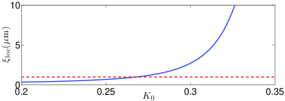
Figure 1: (Color online) The edge localization length $\xi_{\mathrm{loc}}$ for different values of the interaction parameter $K_{0}$. The dashed line marks the length of a micron-sized HgTe QW sample Konig2 .

When $\xi_{\textrm{loc}}<L$, the edge electrons are localized up to temperatures of the order of $\hbar v/(k_{B}\xi_{\mbox{\footnotesize{loc}}})$, with an exponential decrease of the conductivity for lower temperatures GiamarchiSchulz . Thus, the edge remains insulating at the low temperatures (30mK$-$2K) at which experiments are typically carried out Konig .

Having explored the Rashba interaction with a spatially random coupling, one may ask how the QSH edge modes respond to a periodically modulated coupling. The question becomes particularly interesting in light of a proposal by Wang Wang to use a gate-controlled Rashba coupling as a current switch in a quantum wire. As shown in Ref. Wang, , a periodic modulation of a Rashba interaction, produced by a sequence of equally spaced nanosized gates, makes the electrons backscatter coherently and the current gets blocked. By decharging the gates, the current is free to flow again. If this blueprint for a spin transistor can be copied over to the edge of a QSH insulator, one may envision a device enabling fast and efficient control of a dissipationless current.

As a simple model for a periodically modulated Rashba coupling we take $\alpha(x)=A\cos(Qx)$ in Eq. (4) Japaridze . By inspection, the largest effect from this modulation is obtained by choosing $Q=2k_{F}$, as this will produce terms in the integrand where all oscillations are carried by the slowly varying fields $\psi_{\uparrow,\downarrow}$ (with $2k_{F}$ corresponding to a wavelength of roughly $5-10$ nm in a HgTe QW Konig3 ). By considering $K_{0}$ values corresponding to $\xi_{\mbox{\footnotesize{loc}}}>L$ (cf. Fig. 1), we can neglect the intrinsic disordering of the Rashba coupling. Repeating the procedure that took us from Eqs. (1), (2), and (4) to the action in Eq. (7), but now with $\eta(x)$ replaced by the amplitude $A$, we obtain

$$S[\varphi]=\frac{1}{2}\!\int dxd\tau\Big{(}\frac{1}{v}(\partial_{\tau}\varphi)^{2}+v(\partial_{x}\varphi)-2g\cos(\lambda_{K}\varphi)\Big{)},$$

with $g\!\equiv\!A^{2}/(4\pi K\kappa^{2}v)$. This action is that of the well-known quantum sine-Gordon model. The RG flows of $g$ and $K$ are governed by the KT equations $\partial z_{\parallel}/\partial\ell=-z_{\perp}^{2}$ and $\partial z_{\perp}/\partial\ell=-z_{\parallel}z_{\perp}$, with $z_{\parallel}\equiv 4K-2$ and $z_{\perp}\equiv 4g\sqrt{CK^{3}}$, where $C$ is a $\kappa$-dependent constant Giamarchi . When $K_{0}<1/2$, the mass term in the sine-Gordon action is seen to be RG relevant. In this regime backscattering generates a dynamical mass for the edge modes, turning the edge to a Mott insulator. Whether the corresponding mass gap $\Delta$, measured from the Fermi level, is large enough to block the current depends on its size relative to the available thermal energy. To make an estimate for the case of a HgTe QW of length $1\,\mu$m [$20\,\mu$m], we calculate $\Delta$ for three different values of the Rashba amplitude, tuning up the interaction parameter $K_{0}$ until the renormalization length $\kappa\exp(\ell^{*})$ reaches $1\,\mu$m [$20\,\mu$m], with $\exp(\ell^{*})$ the scale factor for which backscattering processes start to dominate (see Fig. 2). When $\kappa\exp(\ell^{*})\approx 1\,\mu$m, $\Delta\approx 4.5\,$meV for all three amplitudes, corresponding to a temperature of around $50$K.

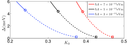
Figure 2: (Color online) The gap $\Delta$ for different Rashba amplitudes $\hbar A$ and values of $K_{0}$ The circles and squares mark the smallest gaps for HgTe QW samples of length $1\,\mu$m and $20\,\mu$m, respectively.

The thermally activated conductance is given by $G=(2e^{2}/h)e^{-\Delta/k_{B}T}$. To prevent thermal leakage of current through the proposed switch, one may thus need to cool a micron-sized sample to temperatures in the range $10-20$ K. For these temperatures our result provides a proof-of-concept of using an ”on-off” modulated Rashba coupling as a switch for QSH edge currents. It should be interesting to repeat our analysis for QWs based on the ternary Heusler compounds Chadov , once these have been put together and characterized. As discussed in Ref. Chadov, , the diversity of Heusler materials opens wide possibilities for tuning the bulk band gap and setting the desired band inversion. This may allow also for enhanced Rashba interactions at the edge. The prospect for a QSH-based spin transistor makes this a promising path to explore.

In summary, we have carried out an analysis of the combined effect of Rashba spin-orbit and e-e interactions on the edge dynamics in a QSH state. The spatial disordering of the Rashba coupling, intrinsic to a quantum well structure that supports a QSH state, is found to localize the edge electrons for sufficiently strong e-e interactions. Likewise, a periodic modulation of the coupling $-$ realizable by placing a configuration of equally spaced nanosized gates on top of the quantum well $-$ localizes the electrons already at intermediate strengths of the e-e interaction. While a practical implementation may have to await advances in nanoscale technology, our result suggests that a Rashba-controlled switch for the dissipationless edge current in a QSH device is a viable possibility. On the more fundamental side, trying to characterize the transition from the Mott insulating phase caused by a periodic Rashba modulation to the Anderson-type localization due to the interplay of e-e interactions and the disordered Rashba coupling remains a challenge.

We thank H. Buhmann, X. Dai, and L. Ioffe for valuable discussions. HJ acknowledges the hospitality of LPTMS, Université de Paris-Sud, for hospitality during the completion of this work. This research was supported by the Swedish Research Council under Grant No. 621-2008-4358 and the Georgian NSF Grant No. ST/09-447.

References

- (1) C. L. Kane and E. J. Mele, Phys. Rev. Lett. 95, 226801 (2005).
- (2) B. A. Bernevig and S.-C. , Phys. Rev. Lett. 96, 106802 (2006).
- (3) For a review, see M. Z. Hasan and C. L. Kane, arXiv:1002.3895.
- (4) M. König et al., Science 318, 766 (2007); A. Roth et al., Science 325, 294 (2009).
- (5) C. Wu et al., Phys. Rev. Lett. 96, 106401 (2006).
- (6) C. Xu and J. E. Moore, Phys. Rev. B 73, 045322 (2006).
- (7) H. Jiang et al., Phys. Rev. Lett. 103, 036803 (2009).
- (8) B. A. Bernevig et al., Science 314, 1757 (2006).
- (9) M. König et al., J. Phys. Soc. Japan 77, 031007 (2008).
- (10) R. Winkler, Spin-Orbit Interaction Effects in Two-Dimensional Electron and Hole Systems (Springer Verlag, Berlin Heidelberg, 2003).
- (11) Y. S. Gui et al., Phys. Rev. B 70, 115328 (2004).
- (12) E. Ya. Sherman, Phys. Rev. B 67, 161303(R) (2003).
- (13) L. E. Golub and E. L. Ivchenko, Phys. Rev. B 69, 115333 (2004).
- (14) A. Ström and H. Johannesson, Phys. Rev. Lett. 102, 096806 (2009).
- (15) M. König et al., Phys. Status Solidi (c) 4, 3374 (2007).
- (16) A. L. Efros and B. I. Shklovskii, Electronic Properties of Doped Semiconductors (Springer, 1989).
- (17) The known second-order spin splitting from a uniform Rashba interaction Wu shows up as a constant shift of the spectrum of the spin-mixed edge modes when treated as a perturbation, with no effect on their propagation.
- (18) T. Giamarchi, Quantum Physics in One Dimension, (Oxford University Press, Oxford, 2003).
- (19) T. Giamarchi and H. J. Schulz, Phys. Rev. B 37, 325 (1988).
- (20) This estimate of agrees with Ref. Chamon, . The larger value in Ref. SJ, stems from an overestimate of screening.
- (21) C.-Y. Hou et al., Phys. Rev. Lett. 102, 076602 (2009).
- (22) X. F. Wang, Phys. Rev. B 69, 035302 (2004).
- (23) G. I. Japaridze et al., Phys. Rev. B 80, 041308(R) (2009).
- (24) S. Chadov et al., arXiv:1003.0193.