Online Sparse System Identification and Signal Reconstruction using Projections onto Weighted $\ell_{1}$ Balls

Abstract.

This paper presents a novel projection-based adaptive algorithm for sparse signal and system identification. The sequentially observed data are used to generate an equivalent sequence of closed convex sets, namely hyperslabs. Each hyperslab is the geometric equivalent of a cost criterion, that quantifies “data mismatch”. Sparsity is imposed by the introduction of appropriately designed weighted $\ell_{1}$ balls. The algorithm develops around projections onto the sequence of the generated hyperslabs as well as the weighted $\ell_{1}$ balls. The resulting scheme exhibits linear dependence, with respect to the unknown system’s order, on the number of multiplications/additions and an $\mathcal{O}(L\log_{2}L)$ dependence on sorting operations, where $L$ is the length of the system/signal to be estimated. Numerical results are also given to validate the performance of the proposed method against the LASSO algorithm and two very recently developed adaptive sparse LMS and LS-type of adaptive algorithms, which are considered to belong to the same algorithmic family.

1. Introduction

Sparsity is the key characteristic of systems whose impulse response consists of only a few nonzero coefficients, while the majority of them retain values of negligible size. Similarly, any signal comprising a small number of nonzero samples is also characterized as being a sparse one. The exploitation of sparsity has been attracting recently an interest of exponential growth under the Compressed Sensing (CS) framework [1, 2, 3]. In principle, CS allows the estimation of sparse signals and systems using fewer measurements than those previously thought to be necessary. More importantly, identification/reconstruction is realized with efficient constrained minimization schemes. Indeed, it has been shown that sparsity is favored by $\ell_{1}$ constrained solutions [4, 5].

With only a few recent exceptions, i.e., [6, 7, 8, 9, 10], the majority of the proposed, so far, CS techniques are appropriate for batch mode operation. In other words, one has to wait until a fixed and predefined number of measurements is available prior to application of CS processing methods, in order to recover the corresponding signal/system estimate. Dynamic online operation for updating and improving estimates, as new measurements become available is not feasible by batch processing methods. The development of efficient, online adaptive CS techniques is of great importance, especially for cases where the signal or system under consideration is time-varying and/or if the available storage resources are limited.

The basic idea in [6, 7] is to use $\ell_{1}$ regularization, i.e., to add to a standard linear or quadratic loss function an extra penalty term expressed by means of the well-known $\ell_{1}$ norm of the unknown system/signal coefficients. Such an approach has been adopted for the classical LMS [6], and for the LS type [7] minimization problems. The resulting recursions for the time update use the current estimate and the information residing in the subgradient of the cost function (due to the non-differentiability of the $\ell_{1}$ norm) to provide the next estimate.

This paper evolves along a different rationale compared to [6, 7], and introduces a projection-based algorithm for sparse system identification and sparse signal reconstruction. The kick-off point is the set theoretic estimation approach, e.g., [11]. Instead of a single optimum, we search for a set of points that are in agreement with the available information, which resides in the training data set (measurements) as well as in the available constraints (the $\ell_{1}$ ball, in this case). To this end, as each new set of measurements is received, a closed convex set is constructed, which defines the region in the solution space that is in “agreement” with the current measurement. In context of the current paper, the shape of these convex sets is chosen to be a hyperslab. The resulting problem is a convex feasibility task, with an infinite number of convex constraints. The fundamental tool of projections onto closed convex sets is used to tackle the problem, following the recent advances on adaptive projection algorithms [12, 13, 14]. Instead of using the information associated with the subgradient of the $\ell_{1}$ norm, the $\ell_{1}$ constraint is imposed on our solution via the exact projection mapping onto a weighted $\ell_{1}$ ball. The algorithm consists of a sequence of projections onto the generated hyperslabs as well as the weighted $\ell_{1}$ balls. The associated complexity is of order $\mathcal{O}(qL)$ multiplications/additions and $\mathcal{O}(L\log_{2}L)$ sorting operations, where $L$ is the length of the system/signal to be identified and $q$ is a user-defined parameter, that controls convergence speed and it defines the number of measurements that are processed, concurrently, at each time instant. The resulting algorithm enjoys a clear geometric interpretation.

The paper is organized as follows. In Section 2 the problem under consideration is described and in Section 3 some definitions and related background are provided. Section 4 presents the proposed algorithm. The derivation and discussion of the projection mapping onto the weighted $\ell_{1}$ ball are treated in Section 5. The adopted mechanism for weighting the $\ell_{1}$ ball is discussed in Section 6. In Section 7, the convergence properties of the algorithm are derived and discussed. It must be pointed out that this section comprises one of the main contributions of the paper, since the existing, so far, theory cannot cover the problem at hand and has to be extended. In Section 8, the performance of the proposed algorithmic scheme is evaluated for both, time-invariant and time-varying scenarios. Section 9 addresses issues related to the sensitivity of the methods, used in the simulations, to non-ideal parametrization and, finally, the conclusions are provided in Section 10. The Appendices offer a more detailed tour to the necessary, for the associated theory, proofs.

2. Problem description

We will denote the set of all integers, non-negative integers, positive integers, and real numbers by $\mathbb{Z},\ \mathbb{Z}_{\geq 0}$, $\mathbb{Z}_{>0}$, and $\mathbb{R}$, respectively. Given two integers $j_{1},j_{2}\in\mathbb{Z}$, such that $j_{1}\leq j_{2}$, let $\overline{j_{1},j_{2}}:=\{j_{1},j_{1}+1,\ldots,j_{2}\}$.

The stage of discussion will be the Euclidean space $\mathbb{R}^{L}$, of dimension $L\in\mathbb{Z}_{>0}$. Its norm will be denoted by $\|{\cdot}\|$. The superscript symbol $(\cdot)^{T}$ will stand for vector transposition. The $\ell_{1}$ norm of a vector $\bm{h}=[h_{1},\ldots,h_{L}]^{T}\in\mathbb{R}^{L}$ is defined as the quantity $\|{\bm{h}}\|_{\ell_{1}}:=\sum_{i=1}^{L}|h_{i}|$. The support of a vector $\bm{h}$ is defined as $\operatorname{supp}(\bm{h}):=\{i\in\overline{1,L}:\ h_{i}\neq 0\}$. The $\ell_{0}$-norm of $\bm{h}$ is defined as the cardinality of its support, i.e., $\|{\bm{h}}\|_{\ell_{0}}:=\#\operatorname{supp}(\bm{h})$.

Put in general terms, the problem to solve is to estimate a vector $\bm{h}_{*}$, based on measurements that are sequentially generated by the (unknown) linear regression model:

$$y_{n}=\bm{x}_{n}^{T}\bm{h}_{*}+v_{n},\forall n\in\mathbb{Z}_{\geq 0},$$ (1)

where the model outputs $(y_{n})_{n\in\mathbb{Z}_{\geq 0}}\subset\mathbb{R}$ and the model input vectors $(\bm{x}_{n})_{n\in\mathbb{Z}_{\geq 0}}\subset\mathbb{R}^{L}$ comprise the measurements and $(v_{n})_{n\in\mathbb{Z}_{\geq 0}}$ is the noise process. Furthermore, the unknown vector $\bm{h}_{*}$ is $S$-sparse, meaning that it has $S$ non-zero terms only, with $S$ being small compared to $L$, i.e., $S:=\|{\bm{h}_{*}}\|_{\ell_{0}}\ll L$.

For a finite number of measurements $N$, the previous data generation model can be written compactly in the following matrix-vector form,

$$\bm{y}=\bm{X}\bm{h}_{*}+\bm{v},$$ (2)

where the input matrix $\bm{X}\in\mathbb{R}^{N\times L}$ has as its rows the input measurement vectors, $\bm{y}:=[y_{1},y_{2},\ldots,y_{N}]^{T}$, and $\bm{v}:=[v_{1},v_{2},\ldots,v_{N}]^{T}$.

Depending on the physical quantity that $\bm{h}_{*}$ represents, the model in (2) suits to both sparse signal reconstruction and linear sparse system identification:

1. Sparse signal reconstruction problem: The aim is to estimate an unknown sparse signal, $\bm{h}_{*}$, based on a set of measurements (training data), that are obtained as inner products of the unknown signal with appropriately selected input vectors, $\bm{x}_{n}$, according to (1). The elements of the input vectors are often selected to be independent and identically distributed (i.i.d.) random variables following, usually, a zero-mean normal or a Bernoulli distribution [5].

2. System identification problem: The unknown sparse system with impulse response $\bm{h}_{*}$ is probed with an input signal $x_{n}$, $n\in\mathbb{Z}_{\geq 0}$ yielding the output values $y_{n}$ as the result of convolution of the input signal with the (unknown) impulse response of the system. In agreement to the model of (1), the measurement (input) vector, at time $n$, is given by $\bm{x}_{n}:=[x_{n},x_{n-1},\ldots,x_{n-L+1}]^{T}$. In the matrix-vector formulation, and for a finite number of measurements, the corresponding measurement matrix $\bm{X}$ is a (partial) Toeplitz one having as entries the elements $\bm{T}_{i,j}=x_{i+L-j}$, where $i\in\overline{1,N}$ and $j\in\overline{1,L}$. The input signal vector, $\bm{x}$, usually consists of i.i.d. normally distributed samples. The study of Toeplitz matrices, with respect to their potential to serve as CS measurement matrices, has been recently intensified, e.g., [15, 16], partially due to their importance in sparse channel estimation applications [17].

A batch approach to estimating a sparse $\bm{h}_{*}$ based on a limited number of measurements $N<L$, is provided by the Least-Absolute Shrinkage and Selection Operator (LASSO):

$$\bm{h}_{*}=\operatorname{arg\,min}_{\bm{h}:\ \|\bm{h}\|_{\ell_{1}}\leq\delta}\|\bm{X}\bm{h}-\bm{y}\|^{2}.$$ (3)

In this case, $\bm{h}_{*}$ is assumed to be stationary and the total number of measurements, $N$, needs to be available prior to solution of the LASSO task.

In the current study, we will assume that $\bm{h}_{*}$ is not only sparse but it is also allowed to be time-varying. This poses certain distinct differences with regard to the standard compressive sampling scenario. The major objective is no longer the estimate of the sparse signal or system, based on a limited number of measurements. The additional requirement, which is often more hard to cope with, is the capability of the estimator to track possible variations of the unknown signal or system. Moreover, this has to take place at an affordable computational complexity, as required by most real time applications, where online adaptive estimation is of interest. Consequently, the batch sparsity aware techniques developed under the CS framework, solving LASSO or one of its variants, become unsuitable under time-varying scenarios. The focus now becomes to develop techniques that a) exploit the sparsity b) exhibit fast convergence to error floors that are as close as possible to those obtained by their batch counterparts c) offer good tracking performance and d) have low computational demands in order to meet the stringent time constraints that are imposed by most real time operation scenarios.

3. Online estimation under the sparsity constraint

The objective of online techniques is the generation of a sequence of estimates, $(\bm{h}_{n})_{n\in\mathbb{Z}_{\geq 0}}$, as time, $n$, evolves, which converge to a value that “best approximates”, in some sense, the unknown sparse vector $\bm{h}_{*}$. The classical approach to this end is to adopt a loss function and then try to minimize it in a time recursive manner. A more recent approach is to achieve the goal via set theoretic arguments by exploiting the powerful tool of projections.

3.1. Loss function minimization approach.

A well-known approach to quantify the “best approximation” term is the minimization of a user-defined loss function

$$\forall n\in\mathbb{Z}_{\geq 0},\forall\bm{h}\in\mathbb{R}^{L},\quad\Theta_{n}(\bm{h}):=\mathcal{L}_{r}^{(n)}(\bm{h})+\gamma_{n}\mathcal{L}_{s}^{(n)}(\bm{h}),$$ (4)

where $\mathcal{L}_{r}^{(n)}$ is computed over the training (observed) data set and accounts for the data mismatch, between measured and desired responses, and $\mathcal{L}_{s}^{(n)}$ accounts for the “size” of the solution, and in the current context is the term that imposes sparsity. The sequence of user-defined parameters $(\gamma_{n})_{n\in\mathbb{Z}_{\geq 0}}$ accounts for the relative contribution of $\mathcal{L}_{r}^{(n)},\mathcal{L}_{s}^{(n)}$ to the cost in (4). Usually, both functions $\mathcal{L}_{r}^{(n)},\mathcal{L}_{s}^{(n)}$ are chosen to be convex, due to the powerful tools offered by the convex analysis theory.

For example, the study in [6] chooses $\mathcal{L}_{r}^{(n)}(\bm{h}):=\frac{1}{2}|y_{n}-\bm{h}^{T}\bm{x}_{n}|^{2}$, where $\mathcal{L}_{s}^{(n)}(\bm{h}):=\|{\bm{h}}\|_{\ell_{1}}$, $\bm{h}\in\mathbb{R}^{L}$, in order to obtain the ZA-LMS algorithm. The RZA-LMS scheme is obtained in [6] when setting $\mathcal{L}_{s}^{(n)}(\bm{h}):=\sum_{i=1}^{L}\log(1+\frac{|h_{i}|}{\eta})$, $\bm{h}\in\mathbb{R}^{L}$, while keeping the same $\mathcal{L}_{r}^{(n)}$. In [7], the sum Least Squares with a forgetting factor $\beta$ is used in place of $\mathcal{L}_{r}^{(n)}$ and the $\ell_{1}$ norm in $\mathcal{L}_{s}^{(n)}$.

3.2. Set theoretic approach.

In this paper, a different path is followed. Instead of attempting to minimize, recursively, a cost function that is defined over the entire observations’ set, our goal becomes to find a set of solutions that is in agreement with the available observations as well as the constraints. To this end, at each time instant, $n$, we require our estimate $\bm{h}_{n}$ to lie within an appropriately defined closed convex set, which is a subset of our solutions space and it is also known as property set. Any point that lies within this set is said to be in agreement with the current measurement pair $(\bm{x}_{n},y_{n})$. The “shape” of the property set is dictated by a “local” loss function, which is assumed to be convex. In the context of the current paper, we have adopted property sets that are defined by the following criterion

$$S_{n}[\epsilon]:=\{\bm{h}\in\mathbb{R}^{L}:\ |\bm{h}^{T}\bm{x}_{n}-y_{n}|\leq\epsilon\},\ n\in\mathbb{Z}_{\geq 0},$$ (5)

for some user-defined tolerance $\epsilon\geq 0$. Such criteria have extensively been used in the context of robust statistics cost functions. Eq. (5) defines a hyperslab, which is indeed a closed convex set. Any point that lies in the hyperslab generated at time $n$ is in agreement with the corresponding measurement at the specific time instance. The parameter $\epsilon$ determines the width of the hyperslabs. Fig. 1 shows two hyperslabs defined at two successive instants, namely, $n$ and $n-1$.

Having associated each measurement pair with a hyperslab, our goal, now, becomes to find a point in $\mathbb{R}^{L}$ that lies in the intersection of these hyperslabs, provided that this is nonempty. We will come back to this point when discussing the convergence issues of our algorithm. For a recent review of this algorithmic family the reader may consult [18].

To exploit sparsity, we adopt the notion of the weighted $\ell_{1}$ norm. Given a vector $\bm{w}_{n}\in\mathbb{R}^{L}$ with positive components, i.e., $w_{n,i}>0$, $\forall i\in\overline{1,L}$, the weighted $\ell_{1}$ ball of radius $\delta>0$ is defined as [19]

$$B_{\ell_{1}}[\bm{w}_{n},\delta]:=\{\bm{h}\in\mathbb{R}^{L}:\ \sum_{i=1}^{L}w_{n,i}|h_{i}|\leq\delta\}.$$ (6)

For more flexibility, we let the weight vector depend on the time instant $n$, hence the notation $\bm{w}_{n}$ has been adopted. We will see later on that such a strategy speeds up convergence and decreases the misadjustment error of the algorithm. The well-known unweighted $\ell_{1}$ ball is nothing but $B_{\ell_{1}}[\bm{1},\delta]$, where $\bm{1}\in\mathbb{R}^{L}$ is a vector with $1$s in all of its components. Note that all the points that lie inside a weighted $\ell_{1}$ norm form a closed convex set.

Having defined the weighted $\ell_{1}$ ball, which is the sparsity related constraint, our task now is to search for a point $\bm{h}$ in $\mathbb{R}^{L}$ that lies in the intersection of the hyperslabs as well as the weighted $\ell_{1}$ balls, i.e., for some $z_{0}\in\mathbb{Z}_{\geq 0}$,

$$\text{find an}\ \bm{h}\in\bigcap_{n\geq z_{0}}\left(S_{n}[\epsilon]\cap B_{\ell_{1}}[\bm{w}_{n},\delta]\right).$$ (7)

As it will become clear later on, when discussing the convergence issues of the algorithm, the existence of $z_{0}$ in (7) allows for a finite number of property sets not to share intersection with the rest.

4. Proposed algorithmic framework

The solution to the problem of finding a point lying in the intersection of a number of closed convex sets has been developed in the context of the classical POCS theory [20, 21, 22, 23], in the case where there is a finite number of sets, and its recent extension, that deals with an infinite number of sets, originally proposed in [12]. The basic idea is very elegant: Keep projecting, according to an appropriate rule, on the involved convex sets; then this sequence of projections will, finally, take you to a point in their intersection. Hence, for our problem, metric projection mapping operators for, both, the hyperslabs as well as the weighted $\ell_{1}$ balls have to be used. Projection operators for hyperslabs are already known and widely used, e.g., [24, 18]. The metric projection mapping onto a weighted $\ell_{1}$ norm will be derived here, and it was presented for a first time, to the best of our knowledge, in [10].

Each time instant, $n$, a new pair of training data $(\bm{x}_{n},y_{n})$ becomes available, and a corresponding hyperslab is formed according to (5). This is used to update the currently available estimate $\bm{h}_{n}$. However, in order to speed up convergence, the update mechanism can also involve previously defined hyperslabs; for example, the hyperslabs formed at time instants $\overline{n-q+1,n}$, for some $q\in\mathbb{Z}_{>0}$. Then, in order to obtain $\bm{h}_{n+1}$, an iteration scheme consisting of three basic steps, is adopted: a) the current estimate $\bm{h}_{n}$ is projected onto each one of the $q$ hyperslabs, b) these projections are in turn combined as a weighted sum and c) the result of the previous step is subsequently projected onto the weighted $\ell_{1}$ ball. This is according to the concepts introduced in [12] and followed in [13, 14, 24]. Schematically, the previous procedure is illustrated in Fig. 1, for the case of $q=2$.

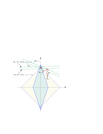
Figure 1. The $\ell_{1}$ ball is shown with dotted lines. At time $n$, the estimate $\bm{h}_{n}$ is available. For $q=2$, two hyperslabs are involved in the update recursion, those associated with time instants $n$ and $n-1$. The new update, $\bm{h}_{n+1}$, results by first projecting $\bm{h}_{n}$ onto the hyperslabs, then combining the resulting projections and finally projecting onto the weighted $\ell_{1}$ norm, that is defined at time $n$ and which is drawn using the full line.

In detail, the algorithm is mathematically described as follows:

Algorithm. Let $q\in\mathbb{Z}_{>0}$, and define the following sliding window on the time axis, of size at most $q$ (to account for the initial period where $n<q-1$), in order to indicate the hyperslabs to be considered at each time instant:

$$\quad\mathcal{J}_{n}:=\overline{\max\{0,n-q+1\},n},\quad\forall n\in\mathbb{Z}_{\geq 0}.$$

For each $n$, define the set of weights $\{\omega_{j}^{(n)}\}_{j\in\mathcal{J}_{n}}\subset(0,1]$ such that $\sum_{j\in\mathcal{J}_{n}}\omega_{j}^{(n)}=1$. Each $\omega_{j}^{(n)}$ quantifies the contribution of the $j$-th hyperslab into the weighted combination of all the hyperslabs that are represented indicated in $\mathcal{J}_{n}$.

Given an arbitrary initial point $\bm{h}_{0}\in\mathbb{R}^{L}$, the following recursion generates the sequence of estimates $(\bm{h}_{n})_{n\in\mathbb{Z}_{\geq 0}}$; $\forall n\in\mathbb{Z}_{\geq 0}$,

$$\bm{h}_{n+1}:=P_{B_{\ell_{1}}[\bm{w}_{n},\delta]}\left(\bm{h}_{n}+\mu_{n}\left(\sum_{j\in\mathcal{J}_{n}}\omega_{j}^{(n)}P_{S_{j}[\epsilon]}(\bm{h}_{n})-\bm{h}_{n}\right)\right),$$ (8)

where $P_{S_{j}[\epsilon]}$ and $P_{B_{\ell_{1}}[\bm{w}_{n},\delta]}$ denote the metric projection mappings onto the hyperslab, defined by the $j$-th data pair, and onto the, (currently available) weighted $\ell_{1}$ ball, respectively. As it will be shown in the analysis of the algorithm in Appendix B, in order to guarantee convergence, the extrapolation parameter $\mu_{n}$ takes values within the interval $(0,2\mathcal{M}_{n})$, where $\mathcal{M}_{n}$ is computed by

$$\mathcal{M}_{n}:=\begin{cases}\frac{\sum_{j\in\mathcal{J}_{n}}\omega_{j}^{(n)}\|{P_{S_{j}[\epsilon]}(\bm{h}_{n})-\bm{h}_{n}}\|^{2}}{\|{\sum_{j\in\mathcal{J}_{n}}\omega_{j}^{(n)}P_{S_{j}[\epsilon]}(\bm{h}_{n})-\bm{h}_{n}}\|^{2}},&\text{if}\ \sum_{j\in\mathcal{J}_{n}}\omega_{j}^{(n)}P_{S_{j}[\epsilon]}(\bm{h}_{n})\neq\bm{h}_{n},\\ 1,&\text{otherwise}.\end{cases}$$ (9)

Notice that the convexity of the function $\|{\cdot}\|^{2}$ implies that $\mathcal{M}_{n}\geq 1$, $\forall n\in\mathbb{Z}_{\geq 0}$.

It is interesting to point out that the algorithm is compactly encoded into a single equation! Also, note that projection onto the $q$ hyperslabs can take place concurrently and this can be exploited if computations are carried our in a parallel processing environment. Moreover, $q$ can be left to vary from iteration to iteration. The dependence of the performance of the algorithm on $q$ will be discussed in Section 8.

It turns out that the projection mappings involved in (8) and (9) have computationally simple forms and are given in (10) and Section 5.2. The algorithm amounts to a computational load of order $\mathcal{O}(qL)$ multiplications/additions and $\mathcal{O}(L\log_{2}L)$ sorting operations. The dependence on $q$ is relaxed in a parallel processing environment.

Having disclosed the algorithmic scheme for the update of our estimate at each iteration step, as measurements are received sequentially, there are a number of issues, yet, to be resolved. First, the involved projection mappings have to be explicitly provided/derived. Second, a strategy for the selection of the weights in the weighted $\ell_{1}$ norm need to be decided. Third, the convergence of the algorithm has to be established. Although the algorithm stands on the shoulders of the theory developed in previously published papers, e.g., [25, 12, 13], the developed, so far, theory is not enough to cover the current algorithm. Since we do not use the $\ell_{1}$ norm, but its weighted version, the projection mapping $P_{B_{\ell_{1}}[\bm{w}_{n},\delta]}$ in (8) is time-varying and it also depends on the obtained estimates. Convergence has to be proved for such a scenario and this is established in Appendix B.

5. Projections onto Closed Convex Sets

A subset $C$ of $\mathbb{R}^{L}$ will be called convex if every line segment $\{\lambda\bm{h}+(1-\lambda)\bm{h}^{\prime}:\lambda\in[0,1]\}$, with endpoints any $\bm{h},\bm{h}^{\prime}\in C$, lies in $C$.

Given any set $C\subset\mathbb{R}^{L}$, define the (metric) distance function $d(\cdot,C):\mathbb{R}^{L}\rightarrow\mathbb{R}$ to $C$ as follows: $\forall\bm{x}\in\mathbb{R}^{L}$, $d(\bm{x},C):=\inf\{\|{\bm{x}-\bm{f}}\|:\ \bm{f}\in C\}$. If we assume now that $C$ is closed and convex, then the (metric) projection onto $C$ is defined as the mapping $P_{C}:\mathbb{R}^{L}\rightarrow C$ which maps to an $\bm{x}\in\mathbb{R}^{L}$ the unique $P_{C}(\bm{x})\in C$ such that $\|{\bm{x}-P_{C}(\bm{x})}\|=d(\bm{x},C)$.

5.1. Projecting onto a hyperslab.

The metric projection operator $P_{S_{n}[\epsilon]}$ onto the hyperslab (5) takes the following simple analytic form [22, 23]:

$$\forall\bm{h}\in\mathbb{R}^{L},\quad P_{S_{n}[\epsilon]}(\bm{h})=\bm{h}+\begin{cases}\frac{y_{n}-\epsilon-\bm{h}^{T}\bm{x}_{n}}{\|{\bm{x}_{n}}\|^{2}}\bm{x}_{n},&\text{if}\ y_{n}-\epsilon>\bm{h}^{T}\bm{x}_{n},\\ \bm{0},&\text{if}\ |\bm{h}^{T}\bm{x}_{n}-y_{n}|\leq\epsilon,\\ \frac{y_{n}+\epsilon-\bm{h}^{T}\bm{x}_{n}}{\|{\bm{x}_{n}}\|^{2}}\bm{x}_{n},&\text{if}\ y_{n}+\epsilon<\bm{h}^{T}\bm{x}_{n}.\end{cases}$$ (10)

5.2. Projecting onto the weighted $\ell_{1}$ ball.

The following theorem computes, in a finite number of steps, the exact projection of a point onto a weighted $\ell_{1}$ ball. The result generalizes the projection mapping computed for the case of the classical unweighted $\ell_{1}$ ball in [26]. In words, the projection mapping exploits the part of the weighted $\ell_{1}$ ball that lies in the non-negative hyperoctant of the associated space. This is because the projection of a point onto the weighted $\ell_{1}$ ball lies always in the same hyperoctant as the point itself. Hence, one may always choose to map the problem on the non-negative hyperoctant, work there, and then return to the original hyperoctant of the space, where the point lies. The part of the weighted $\ell_{1}$ norm, that lies in the non-negative hyperoctant, can be seen as the intersection of a closed halfspace and the non-negative hyperoctant, see Fig. 2. It turns out that if the projection of a point on this specific halfspace has all its components positive, e.g., point $\bm{x}_{1}$ in Fig. 2, then the projection on the halfspace and the projection of the point on the weighted $\ell_{1}$ ball coincide. If, however, some of the components of the projection onto the halfspace are non-positive, e.g., point $\bm{x}_{2}$ in Fig. 2, the corresponding dimensions are ignored and the projection takes place in the resulting lower dimensional space. It turns out that this projection coincides with the projection of the point on the weighted $\ell_{1}$ ball. The previous procedure is formally summarized next.

Figure 2. This figure illustrates the geometry of the weighted $\ell_{1}$ ball $B_{\ell_{1}}[\bm{w},\delta]$, and more specifically its intersection with the non-negative hyperoctant of $\mathbb{R}^{l}$. The reason for studying only the non-negative hyperoctant is justified by Lemma 1. Two points $\bm{x}_{1},\bm{x}_{2}$ of $\mathbb{R}^{l}$ are taken to demonstrate the concepts introduced in the manuscript. Notice that $P_{H_{l}^{-}}(\bm{x}_{1})>\bm{0}$, which implies by Lemma 2.1 that $P_{Q_{l}}(\bm{x}_{1})=P_{H_{l}^{-}}(\bm{x}_{1})$. Notice also the case of $\bm{x}_{2}$ where some components of $P_{H_{l}^{-}}(\bm{x}_{2})$ obtain negative values. Such a case mobilizes Lemma 2.2.

Theorem 1.

Given an $\bm{h}\in\mathbb{R}^{L}\setminus B_{\ell_{1}}[\bm{w}_{n},\delta]$, the following recursion computes, in a finite number of steps (at most $L$), the projection of $\bm{h}$ onto the ball $B_{\ell_{1}}[\bm{w}_{n},\delta]$, i.e., the (unique) vector $P_{B_{\ell_{1}}[\bm{w}_{n},\delta]}(\bm{h})\in\mathbb{R}^{L}$. The case of $\bm{h}\in B_{\ell_{1}}[\bm{w}_{n},\delta]$ is trivial, since $P_{B_{\ell_{1}}[\bm{w}_{n},\delta]}(\bm{h})=\bm{h}$.

1. Form the vector $[|h_{1}|/w_{n,1},\ldots,|h_{L}|/w_{n,L}]^{T}\in\mathbb{R}^{L}$.

2. Sort the previous vector in a non-ascending order (this takes $\mathcal{O}(L\log_{2}L)$ computations), so that $[|h_{\tau(1)}|/w_{n,\tau(1)},\ldots,|h_{\tau(L)}|/w_{n,\tau(L)}]^{T}$, with $|h_{\tau(1)}|/w_{n,\tau(1)}\geq\cdots\geq|h_{\tau(L)}|/w_{n,\tau(L)}$, is obtained. The notation $\tau$ stands for the permutation, which is implicitly defined by the sorting algorithm. Keep in memory the inverse $\tau^{-1}$ which moves the sorted elements back to the original positions.

3. Let $r_{1}:=L$.

4. Let $l=1$. While $l\leq L$, do the following.

   1. Let $\lambda_{*}:=l$.

   2. Find the maximum $j_{*}$ among those $j\in\overline{1,r_{l}}$ such that $\frac{|h_{\tau(j)}|}{w_{n,\tau(j)}}>\frac{\sum_{i=1}^{r_{l}}w_{n,\tau(i)}|h_{\tau(i)}|-\delta}{\sum_{i=1}^{r_{l}}w_{n,\tau(i)}^{2}}$.

   3. If $j_{*}=r_{l}$ then break the loop.

   4. Otherwise, set $r_{l+1}:=j_{*}$.

   5. Increase $l$ by $1$, and go back to Step 4a.

5. Form the vector $\hat{\bm{p}}\in\mathbb{R}^{r_{\lambda_{*}}}$ whose $j$-th component is given by $\hat{p}_{j}:=|h_{\tau(j)}|-\frac{\sum_{i=1}^{r_{\lambda_{*}}}w_{n,\tau(i)}|h_{\tau(i)}|-\delta}{\sum_{i=1}^{r_{\lambda_{*}}}w_{n,\tau(i)}^{2}}w_{n,\tau(j)}$.

6. Use the inverse mapping $\tau^{-1}$, met in step 2, to insert the number $\hat{p}_{j}$ into the $\tau^{-1}(j)$ position of the $L$-dimensional vector $\bm{p}$, i.e., $p_{\tau^{-1}(j)}:=\hat{p}_{j}$, $\forall j\in\overline{1,r_{\lambda_{*}}}$, and fill in the remaining $L-r_{\lambda_{*}}$ positions of $\bm{p}$ with zeros.

7. The desired projection is $P_{B_{\ell_{1}}[\bm{w}_{n},\delta]}(\bm{h})=[\operatorname{sgn}(h_{1})p_{1},\ldots,\operatorname{sgn}(h_{L})p_{L}]^{T}\in\mathbb{R}^{L}$, where the symbol $\operatorname{sgn}(\cdot)$ stands for the sign of a real number.

∎

Proof.

The proof is given in Appendix A. It follows a geometric approach, instead of the Lagrange multipliers methodology, which was followed in [26] for the case of the unweighted $\ell_{1}$ norm. ∎

6. Weighting the $\ell_{1}$ Ball

Motivated by the strategy adopted in [19], the sequence of weights $(\bm{w}_{n})_{n\in\mathbb{Z}_{\geq 0}}$ is designed as follows; let the $i$-th component of the vector $\bm{w}_{n}$ be given by

$$w_{n,i}:=\frac{1}{|h_{n,i}|+\epsilon_{n}^{\prime}},\ \forall i\in\overline{1,L},\ \forall n\in\mathbb{Z}_{\geq 0},$$ (11)

where $(\epsilon^{\prime}_{n})_{n\in\mathbb{Z}_{\geq 0}}$ is a sequence of small positive parameters, which are used in order to avoid division by zero. An illustration of the induced geometry can be seen in Fig. 1. A way to design the parameters $(\epsilon^{\prime}_{n})_{n\in\mathbb{Z}_{\geq 0}}$ will be given in the next section. The corresponding algorithm will be referred to as the Adaptive Projection Algorithm onto Weighted $\ell_{1}$ balls (APWL1). The unweighted case, i.e., when $\bm{w}_{n}:=\bm{1}$, $\forall n\in\mathbb{Z}_{\geq 0}$, will be also considered and is denoted as APL1.

Remark 1.

The radius $\delta$ of the $\ell_{1}$ norm, on which we project, depends on whether the unweighted or the weighted version is adopted. In the unweighted $\ell_{1}$ norm case, the optimum value of the radius is apparently $\delta:=\|{\bm{h}_{*}}\|_{\ell_{1}}$. However, in the weighted case, $\delta$ is set equal to $S=\|{\bm{h}_{*}}\|_{\ell_{0}}$. The reason for this is the following.

Consider the desirable situation where our sequence of estimates $(\bm{h}_{n})_{n\in\mathbb{Z}_{\geq 0}}$ converges to $\bm{h}_{*}$, i.e., $\lim_{n\rightarrow\infty}\bm{h}_{n}=\bm{h}_{*}$. Moreover, let $\epsilon_{n}^{\prime}\geq\epsilon^{\prime}>0$, $\forall n\in\mathbb{Z}_{\geq 0}$, where $\epsilon^{\prime}$ is a user-defined parameter. Then, $\sum_{i=1}^{L}w_{n,i}|h_{n,i}|\leq\sum_{i=1}^{L}\frac{|h_{n,i}|}{|h_{n,i}|+\epsilon^{\prime}}$, $\forall n\in\mathbb{Z}_{\geq 0}$, and thus,

$$\limsup_{n\rightarrow\infty}\sum_{i=1}^{L}w_{n,i}|h_{n,i}| \leq\limsup_{n\rightarrow\infty}\sum_{i=1}^{L}\frac{|h_{n,i}|}{|h_{n,i}|+\epsilon^{\prime}}=\lim_{n\rightarrow\infty}\sum_{i=1}^{L}\frac{|h_{n,i}|}{|h_{n,i}|+\epsilon^{\prime}}$$

$$=\sum_{i\in\operatorname{supp}(\bm{h}_{*})}\frac{|h_{*,i}|}{|h_{*,i}|+\epsilon^{\prime}}+\sum_{i\notin\operatorname{supp}(\bm{h}_{*})}\frac{|h_{*,i}|}{|h_{*,i}|+\epsilon^{\prime}}<\sum_{i\in\operatorname{supp}(\bm{h}_{*})}\frac{|h_{*,i}|}{|h_{*,i}|}=\|{\bm{h}_{*}}\|_{\ell_{0}}.$$

The previous strict inequality and the definition of $\limsup$ suggest that there exists an $m_{1}\in\mathbb{Z}_{\geq 0}$ such that $\forall n\geq m_{1}$ we have $\sum_{i=1}^{L}w_{n,i}|h_{n,i}|\leq\|{\bm{h}_{*}}\|_{\ell_{0}}$. In other words, we obtain that $\forall n\geq m_{1}$, $\bm{h}_{n}\in B_{\ell_{1}}[\bm{w}_{n},\|{\bm{h}_{*}}\|_{\ell_{0}}]$. Hence, a natural choice for $\delta$ in the design of the constraint set $B_{\ell_{1}}[\bm{w}_{n},\delta]$ is $\|{\bm{h}_{*}}\|_{\ell_{0}}$. At least, such a choice is justified $\forall n\geq m_{1}$, since it becomes a necessary condition for having $(\bm{h}_{n})_{n\in\mathbb{Z}_{\geq 0}}$ converge to the desirable $\bm{h}_{*}$.∎

7. Convergence Properties of the Algorithm

It can be shown that, under certain assumptions, the previous algorithm produces a sequence of estimates $(\bm{h}_{n})_{n\in\mathbb{Z}_{\geq 0}}$, which converges to a point located arbitrarily close to an intersection as in (7). The convergence of the algorithm is guaranteed even if a finite number of closed convex sets do not share any nonempty intersection with the rest of the convex constraints in (7). This is important, since it allows for a finite number of data outliers not to disturb the convergence of the algorithm.

Assumptions.

1. Define $\forall n\in\mathbb{Z}_{\geq 0}$, $\Omega_{n}:=B_{\ell_{1}}[\bm{w}_{n},\delta]\cap\left(\bigcap_{j\in\mathcal{J}_{n}}S_{j}[\epsilon]\right)$, i.e., the set $\Omega_{n}$ is defined as the intersection of the weighted $\ell_{1}$ ball and the hyperslabs that are considered at time $n$. Assume that there exists a $z_{0}\in\mathbb{Z}_{\geq 0}$ such that $\Omega:=\bigcap_{n\geq z_{0}}\Omega_{n}\neq\emptyset$. That is, with the exception of a finite number of $\Omega_{n}$s, the rest of them have a nonempty intersection.

2. Choose a sufficiently small $\epsilon^{\prime\prime}>0$, and let $\forall n\in\mathbb{Z}_{\geq 0}$, $\frac{\mu_{n}}{\mathcal{M}_{n}}\in[\epsilon^{\prime\prime},2-\epsilon^{\prime\prime}]$.

3. The interior of $\Omega$ is nonempty, i.e., $\operatorname{int}(\Omega)\neq\emptyset$. For the definition of $\operatorname{int}(\cdot)$ see Fact 2 in Appendix B.

4. Assume that $\check{\omega}:=\inf\{\omega_{j}^{(n)}:\ j\in\mathcal{J}_{n},n\in\mathbb{Z}_{\geq 0}\}>0$. In words, none of the weights, used to combine the projections onto the hyperslabs, will fade away as time $n$ advances.

∎

Theorem 2 (Convergence analysis of the Algorithm).

Under the previously adopted assumptions, the following properties can be established.

1. Every update takes us closer to the intersection $\Omega$. In other words, the convergence is monotonic, that is, $\forall n\geq z_{0}$, $d(\bm{h}_{n+1},\Omega)\leq d(\bm{h}_{n},\Omega)$.

2. Asymptotically, the distance of the obtained estimates from the respective hyperslabs tends to zero. That is, $\lim_{n\rightarrow\infty}\max\{d(\bm{h}_{n},S_{j}[\epsilon]):\ j\in\mathcal{J}_{n}\}=0$.

3. Similarly, the distance of the obtained estimates from the respective weighted $\ell_{1}$ balls tends asymptotically to zero. That is, $\lim_{n\rightarrow\infty}d(\bm{h}_{n},B_{\ell_{1}}[\bm{w}_{n},\delta])=0$.

4. Finally, there exists an $\tilde{\bm{h}}_{*}\in\mathbb{R}^{L}$ such that the sequence of estimates $(\bm{h}_{n})_{n\in\mathbb{Z}_{\geq 0}}$ converges to, i.e., $\lim_{n\rightarrow\infty}\bm{h}_{n}=\tilde{\bm{h}}_{*}$, and that

   $$\tilde{\bm{h}}_{*}\in\left(\overline{\liminf_{n\rightarrow\infty}}B_{\ell_{1}}[\bm{w}_{n},\delta]\right)\cap\left(\overline{\liminf_{n\rightarrow\infty}}\bigcap_{j\in\mathcal{J}_{n}}S_{j}[\epsilon]\right).$$

   Here, $\liminf_{n\rightarrow\infty}C_{n}:=\bigcup_{n\geq 0}\bigcap_{m\geq n}C_{m}$, for any sequence $(C_{n})_{n\in\mathbb{Z}_{\geq 0}}\subset\mathbb{R}^{L}$, and the overline denotes the closure of a set. In other words, the algorithm converges to a point that lies arbitrarily close to an intersection of all the involved property sets.

∎

Proof.

The proof of these results, several auxiliary concepts, as well as details on which assumptions are activated, in order to prove each result, can be found in Appendix B. ∎

Remark 2.

Regarding Assumption 3, the condition $\operatorname{int}\bigcap_{n\in\mathbb{Z}_{\geq 0}}B_{\ell_{1}}[\bm{w}_{n},\delta]\neq\emptyset$ can be easily satisfied. To see this, choose arbitrarily a sufficiently small $\epsilon^{\prime}>0$, and let in (11): $\epsilon^{\prime}_{n}\geq\epsilon^{\prime}$, $\forall n\in\mathbb{Z}_{\geq 0}$. Then, notice by Fig. 2 that $\forall n\in\mathbb{Z}_{\geq 0}$, $\forall i\in\overline{1,L}$, $\frac{\delta}{w_{n,i}}=\delta(|h_{n,i}|+\epsilon_{n}^{\prime})\geq\delta\epsilon_{n}^{\prime}\geq\delta\epsilon^{\prime}$. This clearly implies that $\forall n\in\mathbb{Z}_{\geq 0}$, $B_{\ell_{1}}[\bm{1},\delta\epsilon^{\prime}]\subset B_{\ell_{1}}[\bm{w}_{n},\delta]$, $\forall n\in\mathbb{Z}_{\geq 0}$. It is easy now to verify that $B(\bm{0},\frac{\delta\epsilon^{\prime}}{\sqrt{L}}):=\{\bm{h}\in\mathbb{R}^{L}:\ \|{\bm{h}}\|<\frac{\delta\epsilon^{\prime}}{\sqrt{L}}\}\subset B_{\ell_{1}}[\bm{1},\delta\epsilon^{\prime}]\subset\bigcap_{n\in\mathbb{Z}_{\geq 0}}B_{\ell_{1}}[\bm{w}_{n},\delta]$, which implies, of course, that $\bm{0}\in\operatorname{int}\bigcap_{n\in\mathbb{Z}_{\geq 0}}B_{\ell_{1}}[\bm{w}_{n},\delta]\neq\emptyset$.∎

8. Performance evaluation

In this section, the performance of the proposed algorithms is evaluated against both time-invariant and time-varying signals and systems. It is also compared to a number of other online algorithms such as the Zero-Attracting LMS (ZA-LMS) [6], the Reweighted ZA-LMS (RZA-LMS) [6], and the Recursive LASSO (RLASSO) [7]. Moreover, the LASSO performance, when solved with batch methods [27, 28] is also given, since it serves as a benchmark for the best achievable performance with $\ell_{1}$-regularized LS solvers. All the performance curves are the result from ensemble averaging of 100 independent runs. Moreover, for all the projection based algorithms tested, in all simulation examples, $\mu_{n}$ was set equal to $\mathcal{M}_{n}/2$ and the hyperslabs parameter $\epsilon$ was set equal to $1.3\times\sigma$, with $\sigma$ being the noise standard deviation. Even though such a choice may not be necessarily optimal, the proposed algorithms turn out to be relatively insensitive to the values of these parameters. Finally, $\omega_{j}^{(n)}$ of (8) are set equal to $1/q$, $\forall j\in\mathcal{J}_{n}$, $\forall n\in\mathbb{Z}_{\geq 0}$.

8.1. Time-invariant case.

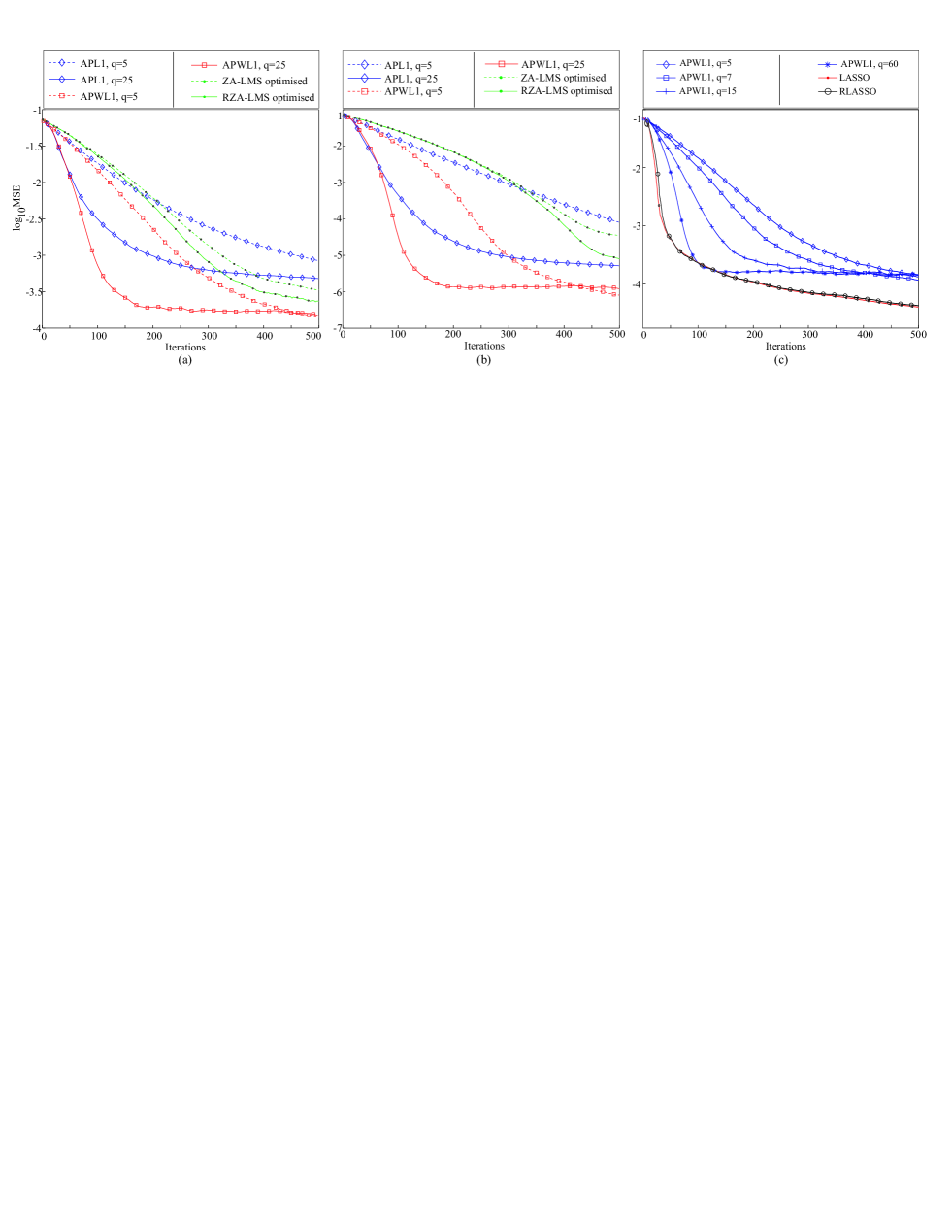
Figure 3. Sparse system identification example with $L=100$ and $S=5$. (a) and (b) shows the performance comparison of the proposed techniques with the LMS-based methods for high and low noise respectively. (c) shows the effect of different $q$ values in comparison to the LASSO performance.

In this simulation example, a time-invariant system having $L=100$ coefficients is used. The system is sparse with $S=5$, i.e., it has only five nonzero coefficients, which are placed in arbitrary positions. The input signal $\bm{x}$ is formed with entries drawn from a zero-mean normal distribution with variance $1$.

In Figs. 3(a) and 3(b) the performance of the new algorithm is compared with that obtained by the LMS-based methods, in different noise levels. The noise variance was set equal to two different values, i.e., $\sigma_{n}^{2}=0.1$ and $\sigma_{n}^{2}=0.001$ corresponding to SNR values of approximately $-3$dB and $17$dB, respectively. Two different values of the parameter $q$ have been considered, namely 5 an 25. Moreover, with respect to the ZA-LMS and the RZA-LMS, the “optimized” tag indicates that the free parameters $\mu$ and $\rho$ were optimized, in order to give the best performance at the 450th iteration. A different parameter setup could lead to faster convergence of both LMS-based methods, albeit at the expense of higher error-floors. In Fig. 3(a) we observe that APWL1 exhibits the best performance both with respect to convergence speed as well as steady-state error floor. In fact, the larger the value of $q$ is the faster the convergence becomes. However, when the unweighted $\ell_{1}$ ball is used (APL1), the method assumes relatively high error-floors, worse than both the LMS-based methods.

In all the cases, unless the contrary is explicitly stated, the adopted values for $\delta$ were: $\delta:=\|{\bm{h}_{*}}\|_{\ell_{1}}$ and $\delta:=S$ for the APL1 and the APWL1 respectively. The sensitivity of these methods, on using different values of $\delta$, will be discussed in section 9.1. Moreover, the adaptation strategy of $\epsilon^{\prime}_{n}$ in (11) was decided upon the following observation. A very small $\epsilon^{\prime}_{n}$, in the range of $[0.001,0.01]$, leads to low error-floors but the convergence speed is compromised. On the other hand, when $\epsilon^{\prime}_{n}$ is relatively large, e.g., $\epsilon^{\prime}_{n}\geq 0.1$, then fast convergence speed is favored at the expense of a higher steady state error floor. In order to tackle this issue efficiently, $\epsilon^{\prime}_{n}$ can start with a high value and then getting gradually smaller. Although other scenarios may be possible, in all the time invariant examples, we have chosen: $\epsilon^{\prime}_{n}:=\epsilon^{\prime}+\frac{1}{n+1}$, $\forall n\in\mathbb{Z}_{\geq 0}$, where $\epsilon^{\prime}$ is a user-defined small positive constant.

Fig. 3(b) corresponds to a low noise level, where the improved performance of the proposed algorithm, compared to that of LMS-based algorithms, is even more enhanced.

It suffices to say, that this enhanced performance is achieved at the expense of higher complexity. The LMS-based algorithms require $O(L)$ multiply/add operations, while the APWL1 demands $q$ times more multiply/add operations. However, in a parallel processing environment, the dependence on $q$ can be relaxed.

In Fig. 3(c) the performance improvement of APWL1, as the $q$ value is increasing, is examined and compared to performance of the RLASSO algorithm. In this system identification case, the $L\times K$ regression matrices, $\bm{H}^{T}_{\tau}$, in [7] are built using the input vectors $(\bm{x}_{n})_{n\in\mathbb{Z}_{\geq 0}}$ according to $[\bm{x}_{L+\tau K-K},\ldots,\bm{x}_{L+\tau K-1}]$, for $\tau\in\mathbb{Z}_{\geq 0}$, and $K\in\mathbb{Z}_{>0}$. Parameter $K$ was set equal to 5. As a reference, the batch LASSO solution is also given, using the true delta value, i.e., $\delta:=\|{\bm{h}_{*}}\|_{\ell_{1}}$. The test is performed for two different noise levels with the solid and the dotted performance curves corresponding to $\sigma_{n}^{2}=0.1$ and $\sigma_{n}^{2}=0.001$. Clearly, the convergence speed rapidly improves as $q$ increases, and the rate of improvement is more noticeable in the range of small values of $q$.

Observe that for large values of $q$, the performance gets “closer” to the one obtained by the LASSO and RLASSO methods. Of course, the larger the $q$ the “heavier” the method becomes from a computationally point of view. However, even for the value of $q=60$ the complexity remains much lower than that of RLASSO. The complexity of the latter algorithm rises up to the order of $\mathcal{O}\left(rL^{2}\right)$, where $r$ is the number of iterations for the cost function minimization in [7, (7)]. Indicatively, in the specific example $r$ needed to be larger than $L$ in order the method to converge for all the realizations that were involved.

In the sequel, we turn our attention to the estimation of a large vector. We will realize it in the context of a signal reconstruction task. We assume a sparse signal vector of 2000 components with $S=20$ arbitrarily positioned nonzero components having values drawn from a zero-mean normal distribution of unit variance. In this case, the observations are obtained from inner products of the unknown signal with independent random measurement vectors, having values distributed according to zero-mean normal distribution of unit variance. The results, are depicted in Fig. 4 for $\sigma_{n}^{2}=0.1$ (SNR=$-10$dB), and $\sigma_{n}^{2}=0.001$ (SNR=$10$dB), drawn with solid and dashed lines, respectively. It is readily observed that the same trend, which was discussed in the previous experiments, holds true for this example. It must be pointed out that in the signal reconstruction task, the input signal may not necessarily have the shift invariance property [29, 30]. Hence, techniques that build around this property and have extensively been used in order to reduce complexity in the context of LS algorithms, are not applicable for such a problem. Both, LMS and the proposed algorithmic scheme do not utilize this property.

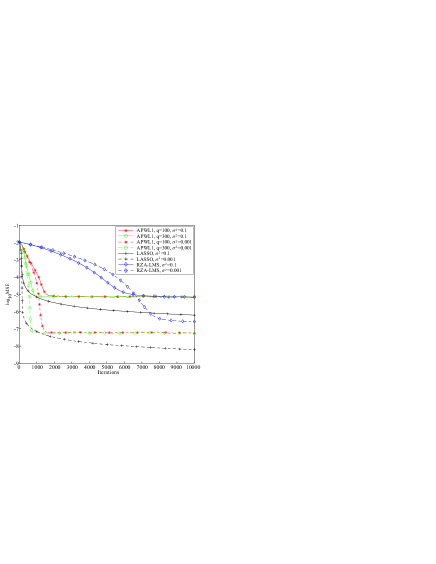
Figure 4. Sparse signal reconstruction example with $L=2000$ and $S=20$, for high and low noise levels.

8.2. Time-varying case.

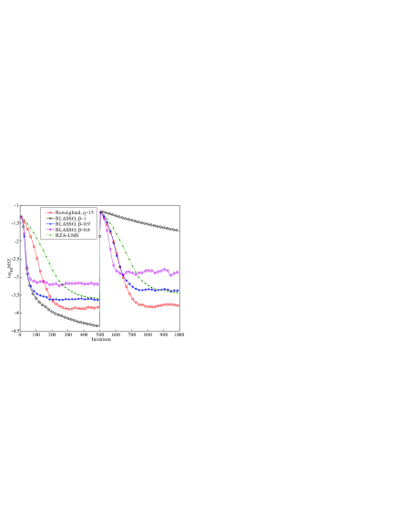
Figure 5. Time-varying sparse system identification example. The system impulse response changes abruptly at iteration $\#501$.

It is by now well established in the adaptive filtering community, e.g., [29], that convergence speed and tracking ability of an algorithm do not, necessarily, follow the same trend. An algorithm may have good converging properties, yet its tracking ability to time variations may not be good, or vice versa. There are many cases where LMS tracks better than the RLS. Although the theoretical analysis of the tracking performance is much more difficult, due to the non-stationarity of the environment, related simulated examples are always needed to demonstrate the performance of an adaptive algorithm in such environments. To this end, in this section, the performance of the proposed method to track time-varying sparse systems is investigated. Both, the number of nonzero elements of $\bm{h}_{*}$ as well as the values of the system’s coefficients are allowed to undergo sudden changes. This is a typical scenario used in adaptive filtering in order to study the tracking performance of an algorithm in practice. The system used in the experiments is 100 coefficients long. The system change is realized as follows: For the first $500$ time instances, the first $5$ coefficients are set equal to 1. Then, at time instance $n=501$ the second and the fourth coefficients are changed to zero, and all the odd coefficients from $\#7$ to $\#15$ are set equal to $1$. Note that the sparsity level, $S$, also changes at time instance $n=501$, and it becomes $8$ instead of $5$. The results are shown in Fig. 5 with the noise variance being set equal to 0.1.

The curve indicated with squares corresponds to the proposed, APWL1 method with $q=15$. The performance of the RLASSO scheme with forgetting factor $\beta=1$ is denoted by circles. The latter clearly outperforms the rest of the methods up to time instance 500. This is expected, since LS-type of algorithms are known to have fast converging properties. Note that up to this time instant, the example coincides with that shown with solid curves in Fig. 3(c). However, the algorithm lucks the “agility” of fast tracking the changes that take place after convergence, due to its long memory. In order to make it track faster, the forgetting factor $\beta$ has to be decreased, in order to “forget” the remote past. However, this affects its (initial) converging properties and in particular the corresponding error floor.

When $\beta=0.8$ (curve denoted by diamonds), the tracking speed of the RLASSO is significantly improved, albeit at the expense of significantly increased error floor. The significant increase in the error floor is also noticed in the first period, where it converges fast, yet to a steady state of increased misadjustment error. Adjusting the $\beta$ parameter to lead to lower error floors, one has to sacrifice tracking speed. For the value of $\beta=0.9$, the RLASSO (curve denoted by stars) achieves the same tracking speed as our proposed method, however its error floor remains notably higher. In fact, the steady state performance of RLASSO in this case, reaches the levels of RZA-LMS (curve denoted by dots).

There are two issues related to the proposed method that have to be discussed for the time-varying case. The first concerns the value of $\delta$ and the other the adaptation strategy of $\epsilon^{\prime}_{n}$. Physical reasoning suggests that $\delta$, for the weighted $\ell_{1}$ ball, should be set equal to $5$ for the first $500$ iterations and then take the value $8$. However, the actual sparsity levels can not be known in advance. As a result, in the example of Fig. 5, $\delta$ was fixed to 9. As it will be discussed soon, the method is rather insensitive against overestimated $\delta$ values. Concerning $\epsilon^{\prime}_{n}$, the adaptation strategy discussed in the previous section, needs a slight modification. Due to the fact that the system undergoes changes, the algorithm has to be alert to track changes. In order to achieve this, the algorithm has the ability to monitor abrupt changes of the orbit $(\bm{h}_{n})_{n\in\mathbb{Z}_{\geq 0}}$. Whenever the estimated impulse response changes considerably, and such a change also appears in the orbit $(\bm{h}_{n})_{n\in\mathbb{Z}_{\geq 0}}$, $\epsilon^{\prime}_{n}$ in (11) is reset to $\epsilon^{\prime}+1$ and it is gradually reduced similarly to the previous example.

9. Sensitivity of APWL1 to Non ideal Parameter Setting

The robustness of any technique is affected by its sensitivity to non “optimized” configurations. In this section, the sensitivity of APWL1 on $\delta$ and $\epsilon$ is examined. The sensitivity of APWL1 is compared to the sensitivity that LASSO and LMS-based algorithms have with respect to their associated parameters.

9.1. Comparing to LASSO

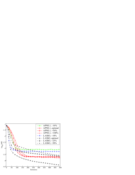
Figure 6. Sensitivity of APWL1 and LASSO to the $\delta$ parameter.

In Fig. 6, the solid lines indicated by diamonds, crosses and circles correspond to the performance of the APWL1, with $q=30$, when the true $\delta$ parameter is overestimated by $50\%$, $100\%$ or underestimated by $10\%$, respectively. The system $\bm{h}_{*}$ under consideration has $L=100$, $S=5$ and $\sigma_{n}^{2}=0.1$. The best performance, drawn with the solid curve indicated with squares, is achieved when the APWL1 method is supplied with the true $\delta$ value, i.e., when $\delta=S$. We observe that the tolerance in $\delta$ underestimation is very limited, since even an underestimation by $10\%$ leads to a significant performance degradation. On the other hand, APWL1 is rather insensitive to overestimation. Indeed, overestimation even by $100\%$, compared to the true value, leads to acceptable results. For comparison, the sensitivity of the standard LASSO is presented with dashed lines. In this case, the optimized $\delta$ value equals to $\|{\bm{h}_{*}}\|_{\ell_{1}}$. The sensitivity of LASSO is clearly higher, particularly to the steady-state region. Observe, that only a $25\%$ deviation from the optimum value (dashed line with diamonds) causes enough performance degradation to bring LASSO at a higher MSE regime, compared APWL1. Moreover, LASSO, similarly to APWL1, exhibits limited tolerance in $\delta$ underestimated $\delta$ values.

9.2. Comparing to LMS-based techniques.

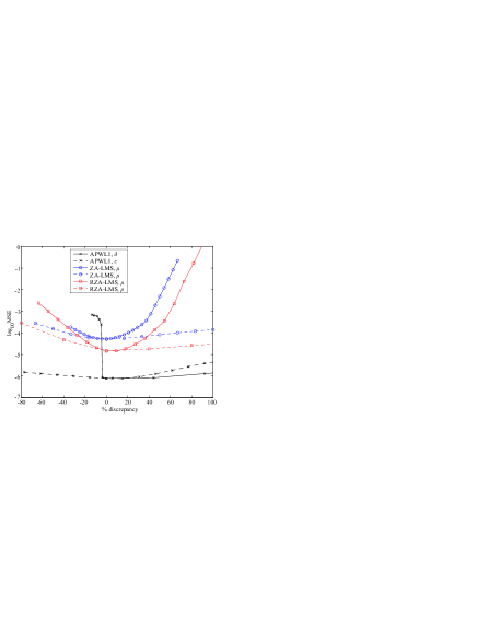
Figure 7. Sensitivity of the LMS-based methods on the $\mu$ and $\rho$ parameters compared to the sensitivity of APWL1 to $\delta$ and $\epsilon$.

Besides the $\delta$ parameter, APWL1 also needs specification of the hyperslabs width, i.e., the parameter $\epsilon$. On the other hand, LMS-based methods need the specification of $\mu$ and $\rho$. Fig. 7 shows the performance degradation of APWL1 (curves with x-crosses), ZA-LMS (curves with circles) and RZA-LMS (curves with rectangles), when they are configured with parameter values which deviate from the “optimum” ones. The x-axis indicates deviation, from the “optimal” values, in percentage. The problem setting is the one shown in Fig. 3(b) and the reported MSE is always evaluated at time instance 450, where convergence is assumed to have been achieved. The $0\%$ discrepancy point, coincides with the best achieved performance of each method. For the LMS-based methods, the solid and dashed curves correspond to $\mu$ and $\rho$, respectively. For the APWL1, the dashed and the solid curves correspond to $\epsilon$ and $\delta$, respectively. Starting with the latter parameter, as expected from the discussion in section 9.1, even a slight underestimation, i.e., negative deviation from the optimum, leads to a sudden performance degradation. On the positive side, the method exhibits a very low sensitivity. With respect to $\epsilon$, the sensitivity of APWL1 is similar to the sensitivity exhibited by the LMS-based methods on the $\rho$ parameter. However, LMS-based methods show an increased sensitivity on the $\mu$ parameter for both negative and positive deviation. In addition, the optimum $\mu$ value depends on the length of $\bm{h}_{*}$, as it is the case with the standard non-regularized LMS [30].

10. Conclusions

A novel efficient algorithm, of linear complexity, for sparse system adaptive identification was presented, based on set theoretic estimation arguments. Sparsity was exploited by the introduction of a sequence of weighted $\ell_{1}$ balls. The algorithm consists of a sequence of projections on hyperslabs, that measure data mismatch with respect to the training data, and on weighted $\ell_{1}$ balls. The projection mapping on a weighted $\ell_{1}$ ball has been derived and a full convergence proof of the algorithm has been established. A comparative performance analysis, using simulated data, was performed against the recently developed online sparse LMS and sparse LS-type of algorithms.

Appendix A The metric projection mapping onto the weighted $\ell_{1}$ ball $B_{\ell_{1}}[\bm{w},\delta]$

The results in this section are stated for any Euclidean space $\mathbb{R}^{l}$, where $l\in\overline{1,L}$. Moreover, given two vectors $\bm{x}:=[x_{1},\ldots,x_{l}]^{T},\bm{y}:=[y_{1},\ldots,y_{l}]^{T}\in\mathbb{R}^{l}$, then the notation $\bm{x}\leq(<)\bm{y}$ means that $\forall i\in\overline{1,l}$, $x_{i}\leq(<)y_{i}$.

A well-known property of the metric projection mapping $P_{C}$ onto a closed convex set $C$, which will be used in the sequel, is the following [22, 23]:

$$\forall\bm{x}\in\mathbb{R}^{l},\forall\bm{f}\in C,\quad\|{\bm{x}-P_{C}(\bm{x})}\|^{2}\leq\|{\bm{x}-\bm{f}}\|^{2}-\|{P_{C}(\bm{x})-\bm{f}}\|^{2}.$$ (12)

Define $Q_{l}:=B_{\ell_{1}}[\bm{w},\delta]\cap\mathbb{R}_{\geq 0}^{l}$, where $\mathbb{R}_{\geq 0}^{l}$ stands for the non-negative hyperoctant of $\mathbb{R}^{l}$ (see Fig. 2). Define also the following closed halfspace: $H_{l}^{-}:=\{\bm{u}\in\mathbb{R}^{l}:\ \sum_{i=1}^{l}w_{i}u_{i}=\bm{w}^{T}\bm{u}\leq\delta\}$. Clearly the boundary of $H_{l}^{-}$ is the hyperplane: $H_{l}:=\{\bm{u}\in\mathbb{R}^{l}:\ \sum_{i=1}^{l}w_{i}u_{i}=\bm{w}^{T}\bm{u}=\delta\}$. It is easy to verify that $Q_{l}=H_{l}^{-}\cap\mathbb{R}_{\geq 0}^{l}$. Clearly, the boundary of $Q_{l}$ is $H_{l}\cap\mathbb{R}_{\geq 0}^{l}$.

Lemma 1.

1. For any $\bm{x}\in\mathbb{R}^{l}$, the projection $P_{B_{\ell_{1}}[\bm{w},\delta]}(\bm{x})$ belongs to the same hyperoctant as $\bm{x}$ does, i.e., if $\bm{x}_{*}:=P_{B_{\ell_{1}}[\bm{w},\delta]}(\bm{x})$, then $\operatorname{sgn}(x_{*,i})=\operatorname{sgn}(x_{i})$, $\forall i\in\overline{1,l}$.

2. Define the mapping $\operatorname{abs}:\bm{x}=[x_{1},\ldots,x_{l}]^{T}\mapsto[|x_{1}|,\ldots,|x_{l}|]^{T}$, $\forall\bm{x}\in\mathbb{R}^{l}$. It can be easily verified that $\operatorname{abs}$ is an one-to-one mapping of any hyperoctant of $\mathbb{R}^{l}$ onto $\mathbb{R}_{\geq 0}^{l}$, i.e., it is a bijection. Fix arbitrarily an $\bm{x}\in\mathbb{R}^{l}$. Consider the mapping $\operatorname{abs}$ which bijectively maps the hyperoctant, in which $\bm{x}$ is located, to $\mathbb{R}_{\geq 0}^{l}$. Then, $P_{B_{\ell_{1}}[\bm{w},\delta]}(\bm{x})=\operatorname{abs}^{-1}\left(P_{B_{\ell_{1}}[\bm{w},\delta]}(\operatorname{abs}(\bm{x}))\right)$, where $\operatorname{abs}^{-1}$ stands for the inverse mapping of $\operatorname{abs}$. In other words, in order to calculate the projection mapping onto $B_{\ell_{1}}[\bm{w},\delta]$, it is sufficient to study only the case of $\mathbb{R}_{\geq 0}^{l}$.

∎

Proof.

1. Without any loss of generality, assume that $\bm{x}$ belongs to the non-negative hyperoctant of $\mathbb{R}^{l}$. We will show that also every component of $\bm{x}_{*}$ is, also, non-negative. In order to derive a contradiction, assume that there exist some negative components of $\bm{x}_{*}$. To make the proof short, and with no loss of generality, assume that the only negative component of $\bm{x}_{*}$ is $x_{*,1}$. Define the vector $\bm{u}_{*}$ such that $u_{*,1}:=0$ and $u_{*,i}:=x_{*,i}$, $\forall i\in\overline{2,l}$. Since $\bm{x}_{*}\in B_{\ell_{1}}[\bm{w},\delta]$, we have that $\sum_{i=1}^{l}w_{i}|x_{*,i}|\leq\delta$, which easily leads to $\sum_{i=1}^{l}w_{i}|u_{*,i}|=\sum_{i=2}^{l}w_{i}|x_{*,i}|\leq\sum_{i=1}^{l}w_{i}|x_{*,i}|\leq\delta$, i.e., $\bm{u}_{*}\in B_{\ell_{1}}[\bm{w},\delta]$. Moreover, notice that since $x_{*,1}<0=u_{*,1}$, then $x_{1}-x_{*,1}>x_{1}-u_{*,1}=x_{1}\geq 0$. Hence, $\|{\bm{x}-\bm{u}_{*}}\|^{2}<(x_{1}-x_{*,1})^{2}+\sum_{i=2}^{l}(x_{i}-x_{*,i})^{2}=\|{\bm{x}-\bm{x}_{*}}\|^{2}$. This contradicts the fact that $\bm{x}_{*}=P_{B_{\ell_{1}}[\bm{w},\delta]}(\bm{x})$, and establishes Lemma 1.1.

2. Fix arbitrarily an $\bm{x}\in\mathbb{R}^{l}$. As we have seen before, $P_{B_{\ell_{1}}[\bm{w},\delta]}(\bm{x})$ will be located in the same hyperoctant as $\bm{x}$. Let any $\bm{u}\in S_{l}$, where $S_{l}$ stands for the intersection of $B_{\ell_{1}}[\bm{w},\delta]$ with the same hyperoctant where $\bm{x}$ belongs to. As a result, we have that $\operatorname{sgn}(x_{i})=\operatorname{sgn}(u_{i})$, $\forall i\in\overline{1,l}$, and

   $$\|{\bm{x}-\bm{u}}\|^{2} =\sum_{i=1}^{l}(x_{i}-u_{i})^{2}=\sum_{i=1}^{l}(\operatorname{sgn}(x_{i})|x_{i}|-\operatorname{sgn}(u_{i})|u_{i}|)^{2}$$

   $$=\sum_{i=1}^{l}(\operatorname{sgn}(x_{i})|x_{i}|-\operatorname{sgn}(x_{i})|u_{i}|)^{2}=\sum_{i=1}^{l}(|x_{i}|-|u_{i}|)^{2}$$

   $$=\|{\operatorname{abs}(\bm{x})-\operatorname{abs}(\bm{u})}\|^{2}.$$

   Notice here that $\operatorname{abs}$ is a bijection from $S_{l}$ to $Q_{l}$, so that the previous equality results into the following:

   $$\|{\operatorname{abs}(\bm{x})-P_{B_{\ell_{1}}[\bm{w},\delta]}(\operatorname{abs}(\bm{x}))}\|=\min_{\bm{u}^{\prime}\in Q_{l}}\|{\operatorname{abs}(\bm{x})-\bm{u}^{\prime}}\|=\min_{\bm{u}\in S_{l}}\|{\operatorname{abs}(\bm{x})-\operatorname{abs}(\bm{u})}\|$$

   $$=\min_{\bm{u}\in S_{l}}\|{\bm{x}-\bm{u}}\|=\|{\bm{x}-P_{B_{\ell_{1}}[\bm{w},\delta]}(\bm{x})}\|=\|{\operatorname{abs}(\bm{x})-\operatorname{abs}\left(P_{B_{\ell_{1}}[\bm{w},\delta]}(\bm{x})\right)}\|.$$

   Therefore, by the uniqueness of the projection, $\operatorname{abs}\left(P_{B_{\ell_{1}}[\bm{w},\delta]}(\bm{x})\right)=P_{B_{\ell_{1}}[\bm{w},\delta]}(\operatorname{abs}(\bm{x}))$, and Lemma 1.2 is established.

∎

Lemma 2.

Let an $\bm{x}\in\mathbb{R}_{\geq 0}^{l}\setminus Q_{l}$, and

$$\bm{x}_{*}:=P_{H_{l}^{-}}(\bm{x})=\bm{x}-\frac{\max\{0,\bm{x}^{T}\bm{w}-\delta\}}{\|{\bm{w}}\|^{2}}\bm{w}.$$ (13)

1. Assume that $\bm{x}_{*}>\bm{0}$. Then, $P_{Q_{l}}(\bm{x})=P_{H_{l}^{-}}(\bm{x})$.

2. Make the following partitions $\bm{x}=\left[\begin{smallmatrix}\hat{\bm{x}}\\ \tilde{\bm{x}}\end{smallmatrix}\right]$, $\bm{x}_{*}=\left[\begin{smallmatrix}\hat{\bm{x}}_{*}\\ \tilde{\bm{x}}_{*}\end{smallmatrix}\right]$, where $\hat{l},\tilde{l}\in\overline{1,l}$, $\hat{l}+\tilde{l}=l$, and $\hat{\bm{x}},\hat{\bm{x}}_{*}\in\mathbb{R}^{\hat{l}}$, $\tilde{\bm{x}},\tilde{\bm{x}}_{*}\in\mathbb{R}^{\tilde{l}}$. Assume, now, that there exists an $\tilde{l}\in\overline{1,l}$ such that $\tilde{\bm{x}}_{*}\leq\bm{0}$. Then,

   $$P_{Q_{l}}(\bm{x})^{T}=[P_{Q_{\hat{l}}}(\hat{\bm{x}})^{T},~{}\bm{0}^{T}]^{T}$$

∎

Proof.

1. Since $\bm{x}_{*}:=P_{H_{l}^{-}}(\bm{x})>\bm{0}$, it is clear that $\bm{x}_{*}\in H_{l}^{-}\cap\mathbb{R}_{\geq 0}^{l}=Q_{l}$. Hence,

   $$\min_{\bm{u}\in Q_{l}}\|{\bm{x}-\bm{u}}\|\leq\|{\bm{x}-\bm{x}_{*}}\|=\|{\bm{x}-P_{H_{l}^{-}}(\bm{x})}\|=\min_{\bm{u}\in H_{l}^{-}}\|{\bm{x}-\bm{u}}\|\leq\min_{\bm{u}\in Q_{l}}\|{\bm{x}-\bm{u}}\|,$$

   where the last inequality comes from $Q_{l}\subset H_{l}^{-}$. Thus, $\|{\bm{x}-P_{H_{l}^{-}}(\bm{x})}\|=\min_{\bm{u}\in Q_{l}}\|{\bm{x}-\bm{u}}\|$. Hence, by the uniqueness of the projection, $P_{Q_{l}}(\bm{x})=P_{H_{l}^{-}}(\bm{x})$, and Lemma 2.1 is established.

2. Since $H_{l}$ is a hyperplane, $\forall\bm{u}\in H_{l}$, $(\bm{u}-\bm{x}_{*})^{T}(\bm{x}-\bm{x}_{*})=0$, which implies, of course, that $\forall\bm{u}\in H_{l}\cap\mathbb{R}_{\geq 0}^{l}$, $(\bm{u}-\bm{x}_{*})^{T}(\bm{x}-\bm{x}_{*})=0$. Thus, $\forall\bm{u}\in H_{l}\cap\mathbb{R}_{\geq 0}^{l}$,

   $$\|{\bm{u}-\bm{x}}\|_{\mathbb{R}^{l}}^{2}=\|{\bm{u}-\bm{x}_{*}}\|_{\mathbb{R}^{l}}^{2}+\|{\bm{x}_{*}-\bm{x}}\|_{\mathbb{R}^{l}}^{2}=\|{\hat{\bm{u}}-\hat{\bm{x}}_{*}}\|_{\mathbb{R}^{\hat{l}}}^{2}+\|{\tilde{\bm{u}}-\tilde{\bm{x}}_{*}}\|_{\mathbb{R}^{\tilde{l}}}^{2}+\|{\bm{x}_{*}-\bm{x}}\|_{\mathbb{R}^{l}}^{2}.$$ (14)

   This in turn implies that

   $$P_{Q_{l}}(\bm{x}) =\operatorname{arg\,min}\{\|{\bm{u}-\bm{x}}\|_{\mathbb{R}^{l}}^{2}:\ \bm{u}\in H_{l}\cap\mathbb{R}_{\geq 0}^{l}\}$$

   $$=\operatorname{arg\,min}\{\|{\bm{u}-\bm{x}}\|_{\mathbb{R}^{l}}^{2}:\ \hat{\bm{u}}\in\mathbb{R}^{\hat{l}}_{\geq 0},\tilde{\bm{u}}\in\mathbb{R}^{\tilde{l}}_{\geq 0},\hat{\bm{u}}^{T}\hat{\bm{w}}+\tilde{\bm{u}}^{T}\hat{\bm{w}}=\delta\}$$

   $$=\operatorname{arg\,min}\{\|{\hat{\bm{u}}-\hat{\bm{x}}_{*}}\|_{\mathbb{R}^{\hat{l}}}^{2}+\|{\tilde{\bm{u}}-\tilde{\bm{x}}_{*}}\|_{\mathbb{R}^{\tilde{l}}}^{2}:\ \hat{\bm{u}}\in\mathbb{R}^{\hat{l}}_{\geq 0},\tilde{\bm{u}}\in\mathbb{R}^{\tilde{l}}_{\geq 0},\hat{\bm{u}}^{T}\hat{\bm{w}}+\tilde{\bm{u}}^{T}\hat{\bm{w}}=\delta\}.$$ (15)

   By our initial assumption $\tilde{\bm{x}}_{*}\leq\bm{0}$. Hence, it is easy to verify that $\forall\hat{\bm{u}}\in\mathbb{R}^{\hat{l}}_{\geq 0}$, $\forall\tilde{\bm{u}}\in\mathbb{R}^{\tilde{l}}_{\geq 0}\setminus\{\bm{0}\}$, $\|{\hat{\bm{u}}-\hat{\bm{x}}_{*}}\|_{\mathbb{R}^{\hat{l}}}^{2}+\|{\bm{0}-\tilde{\bm{x}}_{*}}\|_{\mathbb{R}^{\tilde{l}}}^{2}<\|{\hat{\bm{u}}-\hat{\bm{x}}_{*}}\|_{\mathbb{R}^{\hat{l}}}^{2}+\|{\tilde{\bm{u}}-\tilde{\bm{x}}_{*}}\|_{\mathbb{R}^{\tilde{l}}}^{2}$, which evidently suggests that

   $$\operatorname{arg\,min}\{\|{\hat{\bm{u}}-\hat{\bm{x}}_{*}}\|_{\mathbb{R}^{\hat{l}}}^{2}+\|{\tilde{\bm{u}}-\tilde{\bm{x}}_{*}}\|_{\mathbb{R}^{\tilde{l}}}^{2}:\ \hat{\bm{u}}\in\mathbb{R}^{\hat{l}}_{\geq 0},\tilde{\bm{u}}\in\mathbb{R}^{\tilde{l}}_{\geq 0},\hat{\bm{u}}^{T}\hat{\bm{w}}+\tilde{\bm{u}}^{T}\hat{\bm{w}}=\delta\}$$

   $$\hskip 10.0pt=\operatorname{arg\,min}\{\|{\hat{\bm{u}}-\hat{\bm{x}}_{*}}\|_{\mathbb{R}^{\hat{l}}}^{2}+\|{\tilde{\bm{u}}-\tilde{\bm{x}}_{*}}\|_{\mathbb{R}^{\tilde{l}}}^{2}:\ \hat{\bm{u}}\in\mathbb{R}^{\hat{l}}_{\geq 0},\hat{\bm{u}}^{T}\hat{\bm{w}}=\delta,\tilde{\bm{u}}=\bm{0}\}$$ (16)

   Now, since $\bm{x}\in\mathbb{R}_{\geq 0}^{l}\setminus Q_{l}$, it is clear by the geometry of the $Q_{l}$ that $P_{Q_{l}}(\bm{x})$ will be located on $H_{l}\cap\mathbb{R}_{\geq 0}^{l}$. Hence, by (14), (15), and (16), one can verify the following:

   $$P_{Q_{l}}(\bm{x}) =\operatorname{arg\,min}\{\|{\bm{u}-\bm{x}}\|_{\mathbb{R}^{l}}^{2}:\ \bm{u}\in H_{l}\cap\mathbb{R}_{\geq 0}^{l}\}$$

   $$=\operatorname{arg\,min}\{\|{\hat{\bm{u}}-\hat{\bm{x}}_{*}}\|_{\mathbb{R}^{\hat{l}}}^{2}+\|{\tilde{\bm{u}}-\tilde{\bm{x}}_{*}}\|_{\mathbb{R}^{\tilde{l}}}^{2}:\ \hat{\bm{u}}\in\mathbb{R}^{\hat{l}}_{\geq 0},\tilde{\bm{u}}\in\mathbb{R}^{\tilde{l}}_{\geq 0},\hat{\bm{u}}^{T}\hat{\bm{w}}+\tilde{\bm{u}}^{T}\hat{\bm{w}}=\delta\}$$

   $$=\operatorname{arg\,min}\{\|{\hat{\bm{u}}-\hat{\bm{x}}_{*}}\|_{\mathbb{R}^{\hat{l}}}^{2}+\|{\tilde{\bm{u}}-\tilde{\bm{x}}_{*}}\|_{\mathbb{R}^{\tilde{l}}}^{2}:\ \hat{\bm{u}}\in\mathbb{R}^{\hat{l}}_{\geq 0},\hat{\bm{u}}^{T}\hat{\bm{w}}=\delta,\tilde{\bm{u}}=\bm{0}\}$$

   $$=\operatorname{arg\,min}\{\|{\bm{u}-\bm{x}}\|_{\mathbb{R}^{l}}^{2}:\ \hat{\bm{u}}\in\mathbb{R}^{\hat{l}}_{\geq 0},\hat{\bm{u}}^{T}\hat{\bm{w}}=\delta,\tilde{\bm{u}}=\bm{0}\}$$

   $$=\operatorname{arg\,min}\{\|{\hat{\bm{u}}-\hat{\bm{x}}}\|_{\mathbb{R}^{\hat{l}}}^{2}+\|{\tilde{\bm{u}}-\tilde{\bm{x}}}\|_{\mathbb{R}^{\tilde{l}}}^{2}:\ \hat{\bm{u}}\in\mathbb{R}^{\hat{l}}_{\geq 0},\hat{\bm{u}}^{T}\hat{\bm{w}}=\delta,\tilde{\bm{u}}=\bm{0}\}$$

   $$=\operatorname{arg\,min}\{\|{\hat{\bm{u}}-\hat{\bm{x}}}\|_{\mathbb{R}^{\hat{l}}}^{2}:\ \hat{\bm{u}}\in\mathbb{R}^{\hat{l}}_{\geq 0},\hat{\bm{u}}^{T}\hat{\bm{w}}=\delta,\tilde{\bm{u}}=\bm{0}\}$$

   $$=\operatorname{arg\,min}\{\|{\hat{\bm{u}}-\hat{\bm{x}}}\|_{\mathbb{R}^{\hat{l}}}^{2}:\ \hat{\bm{u}}\in H_{\hat{l}}\cap\mathbb{R}_{\geq 0}^{\hat{l}},\tilde{\bm{u}}=\bm{0}\}$$

   $$=\begin{bmatrix}P_{Q_{\hat{l}}}(\hat{\bm{x}})\\ \bm{0}\end{bmatrix}.$$

   This establishes Lemma 2.2.

∎

Lemma 3.

Assume an $\bm{x}\in\mathbb{R}_{\geq 0}^{l}$ such that $\forall i\in\overline{1,l-1}$, $\frac{x_{i}}{w_{i}}\geq\frac{x_{i+1}}{w_{i+1}}$. Moreover, let $\bm{x}_{*}:=P_{H_{l}^{-}}(\bm{x})$. Assume that there exists an $i_{0}\in\overline{1,l}$ such that $x_{*,i_{0}}\leq 0$. Then, $\forall i\geq i_{0}$, $x_{*,i}\leq 0$.∎

Proof.

Here we consider only the case where $\bm{x}\in\mathbb{R}_{\geq 0}^{l}\setminus Q_{l}$, i.e., $\bm{x}^{T}\bm{w}-\delta>0$. Notice by (13) that

$$x_{*,i}\leq 0\Leftrightarrow\frac{x_{i}}{w_{i}}\leq\frac{\bm{x}^{T}\bm{w}-\delta}{\|{\bm{w}}\|^{2}}.$$ (17)

Now, notice also that by the construction of $\bm{x}$ and by our initial assumption, we have that

$$\forall i\geq i_{0},\quad\frac{x_{i}}{w_{i}}\leq\frac{x_{i_{0}}}{w_{i_{0}}}\leq\frac{\bm{x}^{T}\bm{w}-\delta}{\|{\bm{w}}\|^{2}}.$$

However, by (17), this is equivalent to $x_{*,i}\leq 0$, $\forall i\geq i_{0}$, which establishes Lemma 3. ∎

A.1. The proof of Theorem 1.

Notice that Step 1 is due to Lemma 1. Step 4b refers to the attempt of the algorithm to locate the negative components of a vector, according to Lemma 3. Step 4c refers to Lemma 2.1, while Step 4d corresponds to Lemma 2.2.

Appendix B The proof of Theorem 2

B.1. Preliminaries.

Definition 1 (Subgradient and subdifferential [31]).

Given a convex function $\Theta:\mathbb{R}^{L}\rightarrow\mathbb{R}$, a subgradient $\Theta^{\prime}(\bm{x})$ of $\Theta$ at $\bm{x}\in\mathbb{R}^{L}$ is an element of $\mathbb{R}^{L}$, which satisfies the following property: $\Theta^{\prime}(\bm{x})^{T}(\bm{y}-\bm{x})+\Theta(\bm{x})\leq\Theta(\bm{y})$, $\forall\bm{y}\in\mathbb{R}^{L}$. The set of all the subgradients of $\Theta$ at the point $\bm{x}$ will be called the subdifferential of $\Theta$ at $\bm{x}$, and will be denoted by $\partial\Theta(\bm{x})$. Notice that if $\Theta$ is (Gâteaux) differentiable at $\bm{x}$, then the only subgradient of $\Theta$ at $\bm{x}$ is its differential.∎

Fact 1.

The subdifferential of the metric distance function $d(\cdot,C)$ to a closed convex set $C\subset\mathbb{R}^{L}$ is given as follows [31]:

$$\partial d(\bm{x},C)=\begin{cases}N_{C}(\bm{x})\cap B[\bm{0},1],&\bm{x}\in C,\\ \frac{\bm{x}-P_{C}(\bm{x})}{d(\bm{x},C)},&\bm{x}\notin C,\end{cases}$$

where $N_{C}(\bm{x}):=\{\bm{y}\in\mathbb{R}^{L}:\ \bm{y}^{T}(\bm{f}-\bm{x})\leq 0,\forall\bm{f}\in C\}$, and $B[\bm{0},1]:=\{\bm{y}\in\mathbb{R}^{L}:\ \|{\bm{y}}\|\leq 1\}$. Notice that $\forall\bm{x}\in\mathbb{R}^{L}$, $\|{d^{\prime}(\bm{x},C)}\|\leq 1$, where $d^{\prime}(\bm{x},C)$ stands for any subgradient in $\partial d(\bm{x},C)$.∎

We will give, now, an equivalent description of the Algorithm in (8), which will help us in proving several properties of the algorithm.

Lemma 4 (Equivalent description of the Algorithm in (8)).

Define the following non-negative functions:

$$\forall n\in\mathbb{Z}_{\geq 0},\forall\bm{x}\in\mathbb{R}^{L},\quad\Theta_{n}(\bm{x}):=\begin{cases}\sum_{j\in\mathcal{J}_{n}}\frac{\omega_{j}^{(n)}d(\bm{h}_{n},S_{j}[\epsilon])}{L_{n}}d(\bm{x},S_{j}[\epsilon]),&\text{if}\ \mathcal{I}_{n}\neq\emptyset,\\ 0,&\text{if}\ \mathcal{I}_{n}=\emptyset,\end{cases}$$ (18)

where $\mathcal{I}_{n}:=\{j\in\mathcal{J}_{n}:\ \bm{h}_{n}\notin S_{j}[\epsilon]\}$, and $L_{n}:=\sum_{j\in\mathcal{J}_{n}}\omega_{j}^{(n)}d(\bm{h}_{n},S_{j}[\epsilon])$. Then, (8) can be equivalently written as follows:

$$\forall n\in\mathbb{Z}_{\geq 0},\quad\bm{h}_{n+1}:=\begin{cases}P_{B_{\ell_{1}}[\bm{w}_{n},\delta]}\left(\bm{h}_{n}-\lambda_{n}\frac{\Theta_{n}(\bm{h}_{n})}{\|{\Theta_{n}^{\prime}(\bm{h}_{n})}\|^{2}}\Theta_{n}^{\prime}(\bm{h}_{n})\right),&\text{if}\ \Theta_{n}^{\prime}(\bm{h}_{n})\neq 0,\\ P_{B_{\ell_{1}}[\bm{w}_{n},\delta]}(\bm{h}_{n}),&\text{if}\ \Theta_{n}^{\prime}(\bm{h}_{n})=0,\end{cases}$$ (19)

where $\lambda_{n}\in(0,2)$, $\forall n\in\mathbb{Z}_{\geq 0}$, and $\Theta^{\prime}_{n}(\bm{h}_{n})$ is any subgradient of $\Theta_{n}$ at $\bm{h}_{n}$.∎

Proof.

First, a few comments regarding $L_{n}$ in (18) are in order. It can be easily verified by the definition of $\mathcal{I}_{n}$ that $\exists j_{0}\in\mathcal{J}_{n}:\ \bm{h}_{n}\notin S_{j_{0}}[\epsilon]$, which is in turn equivalent to $d(\bm{h}_{n},S_{j_{0}}[\epsilon])>0$. Hence, $L_{n}\geq\omega_{j_{0}}^{(n)}d(\bm{h}_{n},S_{j_{0}}[\epsilon])>0$, and (18) is well-defined. The reason for introducing $L_{n}$ in the design is to give the freedom to the extrapolation parameter $\mu_{n}$ in (8) to be able to take values greater than or equal to $2$; recall that $\mu_{n}\in(0,2\mathcal{M}_{n})$ and $\mathcal{M}_{n}\geq 1$, $\forall n\in\mathbb{Z}_{\geq 0}$, in (9).

Basic calculus on subdifferentials [31] and the definition of $\mathcal{I}_{n}$ suggest that

$$\partial\Theta_{n}(\bm{x}):=\begin{cases}\sum_{j\in\mathcal{I}_{n}}\frac{\omega_{j}^{(n)}d(\bm{h}_{n},S_{j}[\epsilon])}{L_{n}}\partial d(\bm{x},S_{j}[\epsilon]),&\text{if}\ \mathcal{I}_{n}\neq\emptyset,\\ \{\bm{0}\},&\text{if}\ \mathcal{I}_{n}=\emptyset.\end{cases}$$

Hence, in the case where $\mathcal{I}_{n}\neq\emptyset$, Fact 1 implies that

$$\Theta_{n}^{\prime}(\bm{h}_{n}) =\sum_{j\in\mathcal{I}_{n}}\frac{\omega_{j}^{(n)}d(\bm{h}_{n},S_{j}[\epsilon])}{L_{n}}\frac{\bm{h}_{n}-P_{S_{j}[\epsilon]}(\bm{h}_{n})}{d(\bm{h}_{n},S_{j}[\epsilon])}$$

$$=\frac{1}{L_{n}}\sum_{j\in\mathcal{I}_{n}}\omega_{j}^{(n)}(\bm{h}_{n}-P_{S_{j}[\epsilon]}(\bm{h}_{n}))$$

$$=\frac{1}{L_{n}}\sum_{j\in\mathcal{J}_{n}}\omega_{j}^{(n)}(\bm{h}_{n}-P_{S_{j}[\epsilon]}(\bm{h}_{n})).$$ (20)

Clearly, if $\mathcal{I}_{n}\neq\emptyset$, then $\Theta_{n}^{\prime}(\bm{h}_{n})=\bm{0}\Leftrightarrow\sum_{j\in\mathcal{J}_{n}}\omega_{j}^{(n)}P_{S_{j}[\epsilon]}(\bm{h}_{n})=\bm{h}_{n}$. Notice that the same equivalence holds true also in the case where $\mathcal{I}_{n}=\emptyset$, since in such a case $\bm{h}_{n}\in\bigcap_{j\in\mathcal{J}_{n}}S_{j}[\epsilon]\Leftrightarrow\bm{h}_{n}=P_{S_{j}[\epsilon]}(\bm{h}_{n}),\forall j\in\mathcal{J}_{n}$. In other words, we have derived the following: $\forall n\in\mathbb{Z}_{\geq 0},\Theta_{n}^{\prime}(\bm{h}_{n})=\bm{0}\Leftrightarrow\sum_{j\in\mathcal{J}_{n}}\omega_{j}^{(n)}P_{S_{j}[\epsilon]}(\bm{h}_{n})=\bm{h}_{n}$. By this result, if we substitute (20) in (19), and if we define $\mu_{n}:=\lambda_{n}\mathcal{M}_{n}$, $\forall n\in\mathbb{Z}_{\geq 0}$, where $\mathcal{M}_{n}$ is given in (9), then we obtain the recursion given in (8). ∎

Next are a few observations on the function $\Theta_{n}$, which will help us to establish several convergence properties of the Algorithm in (8). First, notice that

$$\mathcal{I}_{n}=\emptyset\Leftrightarrow\bm{h}_{n}\in\bigcap_{j\in\mathcal{J}_{n}}S_{j}[\epsilon] \Leftrightarrow\left(\omega_{j}^{(n)}\bm{h}_{n}=\omega_{j}^{(n)}P_{S_{j}[\epsilon]}(\bm{h}_{n}),\ \forall j\in\mathcal{J}_{n}\right)$$

$$\Rightarrow\bm{h}_{n}=\sum_{j\in\mathcal{J}_{n}}\omega_{j}^{(n)}P_{S_{j}[\epsilon]}(\bm{h}_{n})\Leftrightarrow\Theta^{\prime}_{n}(\bm{h}_{n})=\bm{0}.$$

In the previous relation, the symbol $\Rightarrow$ becomes $\Leftrightarrow$, if we assume that $\bigcap_{j\in\mathcal{J}_{n}}S_{j}[\epsilon]\neq\emptyset$ [22, Proposition 2.12]. Hence, if $\bigcap_{j\in\mathcal{J}_{n}}S_{j}[\epsilon]\neq\emptyset$, then, $\mathcal{I}_{n}=\emptyset\Leftrightarrow\bm{h}_{n}=\sum_{j\in\mathcal{J}_{n}}\omega_{j}^{(n)}P_{S_{j}[\epsilon]}(\bm{h}_{n})\Leftrightarrow\Theta^{\prime}_{n}(\bm{h}_{n})=\bm{0}$. Moreover, in the case where $\bigcap_{j\in\mathcal{J}_{n}}S_{j}[\epsilon]\neq\emptyset$, one can verify also by the definition of $\Theta_{n}$ that

$$\operatorname{lev_{\leq 0}}\Theta_{n}=\begin{cases}\bigcap_{j\in\mathcal{I}_{n}}S_{j}[\epsilon],&\mathcal{I}_{n}\neq\emptyset,\\ \mathbb{R}^{L},&\mathcal{I}_{n}=\emptyset,\end{cases}$$

where $\operatorname{lev_{\leq 0}}\Theta_{n}:=\{\bm{y}\in\mathbb{R}^{L}:\ \Theta_{n}(\bm{y})\leq 0\}$.

Additionally, in the case where $\bigcap_{j\in\mathcal{J}_{n}}S_{j}[\epsilon]\neq\emptyset$, then we can establish the following equivalency: $\bm{h}_{n}\in\operatorname{lev_{\leq 0}}\Theta_{n}\Leftrightarrow\mathcal{I}_{n}=\emptyset$. This can be proved as follows. For the “$\Leftarrow$” direction, we have that $\mathcal{I}_{n}=\emptyset\Leftrightarrow\bm{h}_{n}\in\bigcap_{j\in\mathcal{J}_{n}}S_{j}[\epsilon]\subset\mathbb{R}^{L}=\operatorname{lev_{\leq 0}}\Theta_{n}$. As for the “$\Rightarrow$” direction, assume for a contradiction that $\mathcal{I}_{n}\neq\emptyset$. Then, by the preceding discussion, we have $\bm{h}_{n}\in\bigcap_{j\in\mathcal{I}_{n}}S_{j}[\epsilon]$, which is an absurd result if we recall the definition of $\mathcal{I}_{n}$. Thus, necessarily, $\mathcal{I}_{n}=\emptyset$, and the claim is proved. In other words, in the case where $\bigcap_{j\in\mathcal{J}_{n}}S_{j}[\epsilon]\neq\emptyset$, then, $\mathcal{I}_{n}=\emptyset\Leftrightarrow\Theta^{\prime}_{n}(\bm{h}_{n})=\bm{0}$, and thus

$$\bm{h}_{n}\in\operatorname{lev_{\leq 0}}\Theta_{n}\Leftrightarrow\Theta^{\prime}_{n}(\bm{h}_{n})=\bm{0}.$$ (21)

Definition 2 (Subgradient projection mapping [32]).

Given a convex function $\Theta:\mathbb{R}^{L}\rightarrow\mathbb{R}$, such that $\operatorname{lev_{\leq 0}}\Theta\neq\emptyset$, define the subgradient projection mapping $T_{\Theta}:\mathbb{R}^{L}\rightarrow\mathbb{R}^{L}$ with respect to $\Theta$ as follows:

$$T_{\Theta}(\bm{x}):=\begin{cases}\bm{x}-\frac{\Theta(\bm{x})}{\|{\Theta^{\prime}(\bm{x})}\|^{2}}\Theta^{\prime}(\bm{x}),&\text{if}\ \bm{x}\notin\operatorname{lev_{\leq 0}}\Theta,\\ \bm{x},&\text{if}\ \bm{x}\in\operatorname{lev_{\leq 0}}\Theta,\end{cases}$$

where $\Theta^{\prime}(\bm{x})$ stands for an arbitrarily fixed subgradient of $\Theta$ at $\bm{x}$. If $I$ stands for the identity mapping in $\mathbb{R}^{L}$, the mapping $T_{\Theta}^{(\lambda)}:=I+\lambda(T_{\Theta}-I)$, $\lambda\in(0,2)$, will be called the relaxed subgradient projection mapping. Moreover, similarly to (12), an important property of $T_{\Theta}^{(\lambda)}$ is the following [32]:

$$\forall\bm{x}\in\mathbb{R}^{L},\forall\bm{f}\in\operatorname{lev_{\leq 0}}\Theta,\quad\frac{2-\lambda}{\lambda}\|{\bm{x}-T_{\Theta}^{(\lambda)}(\bm{x})}\|^{2}\leq\|{\bm{x}-\bm{f}}\|^{2}-\|{T_{\Theta}^{(\lambda)}(\bm{x})-\bm{f}}\|^{2}.$$ (22)

∎

Now, (12) and (22) can be combined as follows.

Lemma 5.

Let a closed convex set $C\subset\mathbb{R}^{L}$, and a convex function $\Theta:\mathbb{R}^{L}\rightarrow\mathbb{R}$ such that $C\cap\operatorname{lev_{\leq 0}}\Theta\neq\emptyset$. Then,

$$\forall\bm{x}\in\mathbb{R}^{L},\forall\bm{f}\in C\cap\operatorname{lev_{\leq 0}}\Theta,\quad\frac{2-\lambda}{2}\|{\bm{x}-P_{C}T_{\Theta}^{(\lambda)}(\bm{x})}\|^{2}\leq\|{\bm{x}-\bm{f}}\|^{2}-\|{P_{C}T_{\Theta}^{(\lambda)}(\bm{x})-\bm{f}}\|^{2}.$$

∎

Proof.

This is a direct consequence of [12, Proposition 1]. ∎

Fact 2 ([12]).

Let a sequence $(\bm{x}_{n})_{n\in\mathbb{Z}_{\geq 0}}\subset\mathbb{R}^{L}$, and a closed convex set $C\subset\mathbb{R}^{L}$. Assume that

$$\exists\kappa>0:\ \forall\bm{f}\in C,\ \forall n\in\mathbb{Z}_{\geq 0},\quad\kappa\|{\bm{x}_{n+1}-\bm{x}_{n}}\|^{2}\leq\|{\bm{x}_{n}-\bm{f}}\|^{2}-\|{\bm{x}_{n+1}-\bm{f}}\|^{2}.$$

Assume, also, that there exists a hyperplane $\Pi$ such that the relative interior of the set $C$ with respect to $\Pi$ is nonempty, i.e., $\operatorname{ri}_{\Pi}C\neq\emptyset$. Then, $\exists\bm{x}_{*}\in\mathbb{R}^{L}:\ \bm{x}_{*}=\lim_{n\rightarrow\infty}\bm{x}_{n}$.

Here, given any $\Upsilon\subset\mathbb{R}^{L}$, $\operatorname{ri}_{\Upsilon}C:=\{\bm{y}\in\mathbb{R}^{L}:\ \exists\rho>0,B(\bm{y},\rho)\cap\Upsilon\subset C\}$. As a byproduct of this definition, the interior of $C$ is defined as $\operatorname{int}C:=\operatorname{ri}_{\mathbb{R}^{L}}C$. Hence, it becomes clear that if $\operatorname{int}C\neq\emptyset$, then we can always find a hyperplane $\Pi\subset\mathbb{R}^{L}$ such that $\operatorname{ri}_{\Pi}C\neq\emptyset$. This fact will be used in the proof of Theorem 2.4.∎

Fact 3 ([12]).

Let $C\subset\mathbb{R}^{L}$ be a nonempty closed convex set. Assume also an $\mathring{\bm{f}}\in\operatorname{int}C$, i.e., $\exists\rho>0$ such that $B(\mathring{\bm{f}},\rho)\subset C$. Assume, now, an $\bm{x}\in\mathbb{R}^{L}\setminus C$, and a $t\in(0,1)$ such that $\mathring{\bm{f}}+t(\bm{x}-\mathring{\bm{f}})\notin C$. Then, $d(\bm{x},C)>\rho\frac{1-t}{t}$.∎

Lemma 6.

The set of all subgradients of the collection of convex functions $(\Theta_{n})_{n\in\mathbb{Z}_{\geq 0}}$, defined in (18), is bounded, i.e., $\forall n\in\mathbb{Z}_{\geq 0}$, $\forall\bm{x}\in\mathbb{R}^{L}$, $\|{\Theta_{n}^{\prime}(\bm{x})}\|\leq 1$.∎

Proof.

Fix arbitrarily an $n\in\mathbb{Z}_{\geq 0}$. Here we deal only with the case $\mathcal{I}_{n}\neq\emptyset$, since otherwise, the function $\Theta_{n}$ becomes everywhere zero, and for such a function, Lemma 6 holds trivially.

By (18), Fact 1, and some calculus on subdifferentials [31], we obtain that $\forall\bm{x}\in\mathbb{R}^{L}$, the norm of any subgradient $\Theta_{n}^{\prime}(\bm{x})$ satisfies the following:

$$\|{\Theta_{n}^{\prime}(\bm{x})}\| =\|{\sum_{j\in\mathcal{I}_{n}}\frac{\omega_{j}^{(n)}d(\bm{h}_{n},S_{j}[\epsilon])}{L_{n}}d^{\prime}(\bm{x},S_{j}[\epsilon])}\|$$

$$=\|{\sum_{j\in\mathcal{J}_{n}}\frac{\omega_{j}^{(n)}d(\bm{h}_{n},S_{j}[\epsilon])}{L_{n}}d^{\prime}(\bm{x},S_{j}[\epsilon])}\|$$

$$\leq\sum_{j\in\mathcal{J}_{n}:\ \bm{x}\notin S_{j}[\epsilon]}\frac{\omega_{j}^{(n)}d(\bm{h}_{n},S_{j}[\epsilon])}{L_{n}}\|{d^{\prime}(\bm{x},S_{j}[\epsilon])}\|$$

$$\hskip 50.0pt+\sum_{j\in\mathcal{J}_{n}:\ \bm{x}\in S_{j}[\epsilon]}\frac{\omega_{j}^{(n)}d(\bm{h}_{n},S_{j}[\epsilon])}{L_{n}}\|{d^{\prime}(\bm{x},S_{j}[\epsilon])}\|$$

$$\leq\sum_{j\in\mathcal{J}_{n}:\ \bm{x}\notin S_{j}[\epsilon]}\frac{\omega_{j}^{(n)}d(\bm{h}_{n},S_{j}[\epsilon])}{L_{n}}\frac{\|{\bm{x}-P_{S_{j}[\epsilon]}(\bm{x})}\|}{d(\bm{x},S_{j}[\epsilon])}+\sum_{j\in\mathcal{J}_{n}:\ \bm{x}\in S_{j}[\epsilon]}\frac{\omega_{j}^{(n)}d(\bm{h}_{n},S_{j}[\epsilon])}{L_{n}}$$

$$=\sum_{j\in\mathcal{J}_{n}:\ \bm{x}\notin S_{j}[\epsilon]}\frac{\omega_{j}^{(n)}d(\bm{h}_{n},S_{j}[\epsilon])}{L_{n}}+\sum_{j\in\mathcal{J}_{n}:\ \bm{x}\in S_{j}[\epsilon]}\frac{\omega_{j}^{(n)}d(\bm{h}_{n},S_{j}[\epsilon])}{L_{n}}=1.$$

This establishes Lemma 6. ∎

B.2. The proof of Theorem 2.

1. Assumption 1, Definition 2, and (21) suggest that (19) can be equivalently written as follows: $\forall n\geq z_{0}$, $\bm{h}_{n+1}=P_{B_{\ell_{1}}[\bm{w}_{n},\delta]}T_{\Theta_{n}}^{(\lambda_{n})}(\bm{h}_{n})$, where $T_{\Theta_{n}}^{(\lambda_{n})}$ stands for the relaxed subgradient projection mapping with respect to $\Theta_{n}$. Notice here that $\forall n\geq z_{0}$, $\operatorname{lev_{\leq 0}}\Theta_{n}=\bigcap_{j\in\mathcal{I}_{n}}S_{j}[\epsilon]\supset\bigcap_{j\in\mathcal{J}_{n}}S_{j}[\epsilon]$. Thus, by Assumption 1 and Lemma 5, we have that $\forall n\geq z_{0},\forall\bm{f}\in\Omega$,

   $$0 \leq\frac{2-\lambda_{n}}{2}\|{\bm{h}_{n}-\bm{h}_{n+1}}\|^{2}=\frac{2-\lambda_{n}}{2}\|{\bm{h}_{n}-P_{B_{\ell_{1}}[\bm{w}_{n},\delta]}T_{\Theta_{n}}^{(\lambda_{n})}(\bm{h}_{n})}\|^{2}$$

   $$\leq\|{\bm{h}_{n}-\bm{f}}\|^{2}-\|{P_{B_{\ell_{1}}[\bm{w}_{n},\delta]}T_{\Theta_{n}}^{(\lambda_{n})}(\bm{h}_{n})-\bm{f}}\|^{2}=\|{\bm{h}_{n}-\bm{f}}\|^{2}-\|{\bm{h}_{n+1}-\bm{f}}\|^{2}$$ (23)

   $$\Rightarrow\|{\bm{h}_{n+1}-\bm{f}}\|\leq\|{\bm{h}_{n}-\bm{f}}\|.$$ (24)

   If we apply $\inf_{\bm{f}\in\Omega}$ on both sides of (24), we establish our original claim.

2. The next claim is to show that under Assumption 1, the sequence $(\|{\bm{h}_{n}-\bm{f}}\|)_{n\in\mathbb{Z}_{\geq 0}}$ converges $\forall\bm{f}\in\Omega$. To this end, fix arbitrarily $\bm{f}\in\Omega$. By (24), the sequence $(\|{\bm{h}_{n}-\bm{f}}\|)_{n\geq z_{0}}$ is non-increasing, and bounded below. Hence, it is convergent. This establishes the claim.

   Next we will show that under Assumption 1, the set of all cluster points of the sequence $(\bm{h}_{n})_{n\in\mathbb{Z}_{\geq 0}}$ is nonempty, i.e., $\mathfrak{C}((\bm{h}_{n})_{n\in\mathbb{Z}_{\geq 0}})\neq\emptyset$.

   We will first show that the sequence $(\bm{h}_{n})_{n\in\mathbb{Z}_{\geq 0}}$ is bounded. This can be easily verified as follows; fix arbitrarily an $\bm{f}\in\Omega$ and notice that $\forall n\geq z_{0}$, $\|{\bm{h}_{n}}\|\leq\|{\bm{h}_{n}-\bm{f}}\|+\|{\bm{f}}\|\leq\|{\bm{h}_{z_{0}}-\bm{f}}\|+\|{\bm{f}}\|$. Define now $D:=\max\{\|{\bm{h}_{z_{0}}-\bm{f}}\|+\|{\bm{f}}\|,\|{\bm{h}_{0}}\|,\ldots,\|{\bm{h}_{z_{0}-1}}\|\}$, which clearly implies that $\forall n\in\mathbb{Z}_{\geq 0}$, $\|{\bm{h}_{n}}\|\leq D$. Since $(\bm{h}_{n})_{n\in\mathbb{Z}_{\geq 0}}$ is bounded, there exists a subsequence of $(\bm{h}_{n})_{n\in\mathbb{Z}_{\geq 0}}$ which converges to an $\tilde{\bm{h}}_{*}\in\mathbb{R}^{L}$ (Bolzano-Weierstrass Theorem). Hence, $\tilde{\bm{h}}_{*}\in\mathfrak{C}((\bm{h}_{n})_{n\in\mathbb{Z}_{\geq 0}})\neq\emptyset$. This establishes the claim.

   Let Assumptions 1 and 2 hold true. Then, we will show that $\lim_{n\rightarrow\infty}\Theta_{n}(\bm{h}_{n})=0$. First, we will prove that

   $$\lim_{n\rightarrow\infty}\frac{\Theta_{n}(\bm{h}_{n})}{\|{\Theta^{\prime}_{n}(\bm{h}_{n})}\|}=0.$$ (25)

   We will show this by deriving a contradiction. To this end, assume that there exists a $\delta>0$ and a subsequence $(n_{k})_{k\in\mathbb{Z}_{\geq 0}}$ such that $\forall k\in\mathbb{Z}_{\geq 0}$, $\frac{\Theta_{n_{k}}(\bm{h}_{n_{k}})}{\|{\Theta^{\prime}_{n_{k}}(\bm{h}_{n_{k}})}\|}\geq\delta$. We can always choose a sufficiently large $k_{0}$ such that $\forall k\geq k_{0}$, $n_{k}\geq z_{0}$.

   Let, now, any $\bm{f}\in\Omega$, and recall that $\Omega\subset B_{\ell_{1}}[\bm{w}_{n_{k}},\delta]$, $\forall k\geq k_{0}$. Then, verify that the following holds true $\forall k\geq k_{0}$:

   $$\|{\bm{h}_{n_{k}+1}-\bm{f}}\|^{2}=\|{P_{B_{\ell_{1}}[\bm{w}_{n_{k}},\delta]}\left(\bm{h}_{n_{k}}-\lambda_{n_{k}}\frac{\Theta_{n_{k}}(\bm{h}_{n_{k}})}{\|{\Theta_{n_{k}}^{\prime}(\bm{h}_{n_{k}})}\|^{2}}\Theta_{n_{k}}^{\prime}(\bm{h}_{n_{k}})\right)-\bm{f}}\|^{2}$$

   $$\leq\|{\bm{h}_{n_{k}}-\lambda_{n_{k}}\frac{\Theta_{n_{k}}(\bm{h}_{n_{k}})}{\|{\Theta_{n_{k}}^{\prime}(\bm{h}_{n_{k}})}\|^{2}}\Theta_{n_{k}}^{\prime}(\bm{h}_{n_{k}})-\bm{f}}\|^{2}$$

   $$=\|{\bm{h}_{n_{k}}-\bm{f}}\|^{2}+\lambda_{n_{k}}^{2}\frac{\Theta_{n_{k}}^{2}(\bm{h}_{n_{k}})}{\|{\Theta_{n_{k}}^{\prime}(\bm{h}_{n_{k}})}\|^{2}}-2\lambda_{n_{k}}\frac{\Theta_{n_{k}}(\bm{h}_{n_{k}})}{\|{\Theta_{n_{k}}^{\prime}(\bm{h}_{n_{k}})}\|^{2}}{\Theta_{n_{k}}^{\prime}(\bm{h}_{n_{k}})}^{T}(\bm{h}_{n_{k}}-\bm{f}),$$ (26)

   where (12) was used for $P_{B_{\ell_{1}}[\bm{w}_{n_{k}},\delta]}$ in order to derive the previous inequality. By the definition of the subgradient, we have that ${\Theta_{n_{k}}^{\prime}(\bm{h}_{n_{k}})}^{T}(\bm{f}-\bm{h}_{n_{k}})+\Theta_{n_{k}}(\bm{h}_{n_{k}})\leq\Theta_{n_{k}}(\bm{f})=0$. If we merge this into (26), we obtain the following:

   $$\|{\bm{h}_{n_{k}+1}-\bm{f}}\|^{2} \leq\|{\bm{h}_{n_{k}}-\bm{f}}\|^{2}+\lambda_{n_{k}}^{2}\frac{\Theta_{n_{k}}^{2}(\bm{h}_{n_{k}})}{\|{\Theta_{n_{k}}^{\prime}(\bm{h}_{n_{k}})}\|^{2}}-2\lambda_{n_{k}}\frac{\Theta_{n_{k}}^{2}(\bm{h}_{n_{k}})}{\|{\Theta_{n_{k}}^{\prime}(\bm{h}_{n_{k}})}\|^{2}}$$

   $$=\|{\bm{h}_{n_{k}}-\bm{f}}\|^{2}-\lambda_{n_{k}}(2-\lambda_{n_{k}})\frac{\Theta_{n_{k}}^{2}(\bm{h}_{n_{k}})}{\|{\Theta_{n_{k}}^{\prime}(\bm{h}_{n_{k}})}\|^{2}}.$$

   This, in turn, implies that

   $$\forall k\geq k_{0},\quad 0<(\epsilon^{\prime\prime}\delta)^{2}\leq\lambda_{n_{k}}(2-\lambda_{n_{k}})\frac{\Theta_{n_{k}}^{2}(\bm{h}_{n_{k}})}{\|{\Theta_{n_{k}}^{\prime}(\bm{h}_{n_{k}})}\|^{2}}\leq\|{\bm{h}_{n_{k}}-\bm{f}}\|^{2}-\|{\bm{h}_{n_{k}+1}-\bm{f}}\|^{2}.$$ (27)

   However, as we have already shown before, $(\|{\bm{h}_{n}-\bm{f}}\|)_{n\in\mathbb{Z}_{\geq 0}}$ is convergent, and hence it is a Cauchy sequence. This implies that $\lim_{k\rightarrow\infty}(\|{\bm{h}_{n_{k}}-\bm{f}}\|^{2}-\|{\bm{h}_{n_{k}+1}-\bm{f}}\|^{2})=0$, which apparently contradicts (27). In other words, (25) holds true.

   Notice, now, that for all those $n\in\mathbb{Z}_{\geq 0}$ such that $\Theta_{n}^{\prime}(\bm{h}_{n})\neq 0$, we have by Lemma 6 that

   $$\Theta_{n}(\bm{h}_{n})=\|{\Theta_{n}^{\prime}(\bm{h}_{n})}\|\frac{\Theta_{n}(\bm{h}_{n})}{\|{\Theta_{n}^{\prime}(\bm{h}_{n})}\|}\leq\frac{\Theta_{n}(\bm{h}_{n})}{\|{\Theta_{n}^{\prime}(\bm{h}_{n})}\|}.$$ (28)

   Notice, also, here that for all those $n\in\mathbb{Z}_{\geq 0}$ such that $\Theta_{n}^{\prime}(\bm{h}_{n})=0$, it is clear by the well-known fact $\bm{0}\in\partial\Theta_{n}(\bm{h}_{n})\Leftrightarrow\bm{h}_{n}\in\operatorname{arg\,min}\{\Theta_{n}(\bm{x}):\ \bm{x}\in\mathbb{R}^{L}\}$ that $\Theta_{n}(\bm{h}_{n})=0$. Take $\lim_{n\rightarrow\infty}$ on both sides of (28), and use (25) to establish our original claim.

   Let now Assumption 1 holds true. Then we show that there exists a $D>0$ such that $\forall n\in\mathbb{Z}_{\geq 0}$, $L_{n}\leq D$. Notice, that $\forall n\geq z_{0}$, $\forall j\in\mathcal{J}_{n}$, $\forall\bm{f}\in\Omega$,

   $$d(\bm{h}_{n},S_{j}[\epsilon]) =\|{\bm{h}_{n}-P_{S_{j}[\epsilon]}(\bm{h}_{n})}\|\leq\|{\bm{h}_{n}-\bm{f}}\|+\|{\bm{f}-P_{S_{j}[\epsilon]}(\bm{h}_{n})}\|$$

   $$\leq 2\|{\bm{h}_{n}-\bm{f}}\|\leq 2\|{\bm{h}_{z_{0}}-\bm{f}}\|,$$

   where we have used (12) and the monotonicity of the sequence $(\|{\bm{h}_{n}-\bm{f}}\|)_{n\geq z_{0}}$. Then, by the definition of $L_{n}$,

   $$\forall n\geq z_{0},\quad L_{n}=\sum_{j\in\mathcal{J}_{n}}\omega_{j}^{(n)}d(\bm{h}_{n},S_{j}[\epsilon])\leq 2\sum_{j\in\mathcal{J}_{n}}\omega_{j}^{(n)}\|{\bm{h}_{z_{0}}-\bm{f}}\|=2\|{\bm{h}_{z_{0}}-\bm{f}}\|.$$

   Choose, now, any $D>\max\{2\|{\bm{h}_{z_{0}}-\bm{f}}\|,L_{0},\ldots,L_{z_{0}-1}\}\geq 0$, and notice that for such a $D$ the claim holds true.

   Let Assumptions 1, 2, and 4 hold true. By (18), we observe that

   $$\frac{D}{\check{\omega}}\Theta_{n}(\bm{h}_{n}) =\frac{D}{\check{\omega}}\sum_{j\in\mathcal{J}_{n}}\frac{\omega_{j}^{(n)}d^{2}(\bm{h}_{n},S_{j}[\epsilon])}{L_{n}}\geq\frac{D}{\check{\omega}}\sum_{j\in\mathcal{J}_{n}}\frac{\omega_{j}^{(n)}d^{2}(\bm{h}_{n},S_{j}[\epsilon])}{D}$$

   $$\geq\frac{D}{\check{\omega}}\frac{\check{\omega}}{D}\sum_{j\in\mathcal{J}_{n}}d^{2}(\bm{h}_{n},S_{j}[\epsilon])\geq\max\{d^{2}(\bm{h}_{n},S_{j}[\epsilon]):\ j\in\mathcal{J}_{n}\}.$$

   Hence, if we take $\lim_{n\rightarrow\infty}$ on both sides of the previous inequality, we establish Theorem 2.2.

3. Here we establish Theorem 2.3. Let Assumptions 1 and 2 hold true. We utilize first (12) and then (22) in order to obtain the following: $\forall\bm{f}\in\Omega$,

   $$\|{(I-P_{B_{\ell_{1}}[\bm{w}_{n},\delta]})(T_{\Theta_{n}}^{(\lambda_{n})}(\bm{h}_{n}))}\|^{2}\leq\|{T_{\Theta_{n}}^{(\lambda_{n})}(\bm{h}_{n})-\bm{f}}\|^{2}-\|{P_{B_{\ell_{1}}[\bm{w}_{n},\delta]}T_{\Theta_{n}}^{(\lambda_{n})}(\bm{h}_{n})-\bm{f}}\|^{2}$$

   $$=\|{T_{\Theta_{n}}^{(\lambda_{n})}(\bm{h}_{n})-\bm{f}}\|^{2}-\|{\bm{h}_{n+1}-\bm{f}}\|^{2}$$

   $$\leq\|{\bm{h}_{n}-\bm{f}}\|^{2}-\frac{2-\lambda_{n}}{\lambda_{n}}\|{\bm{h}_{n}-T_{\Theta_{n}}^{(\lambda_{n})}(\bm{h}_{n})}\|^{2}-\|{\bm{h}_{n+1}-\bm{f}}\|^{2}\leq\|{\bm{h}_{n}-\bm{f}}\|^{2}-\|{\bm{h}_{n+1}-\bm{f}}\|^{2}.$$

   Take $\lim_{n\rightarrow\infty}$ on both sides of this inequality and recall that the sequence $(\|{\bm{h}_{n}-\bm{f}}\|)_{n\in\mathbb{Z}_{\geq 0}}$ is convergent, and thus Cauchy, in order to obtain

   $$\lim_{n\rightarrow\infty}\|{(I-P_{B_{\ell_{1}}[\bm{w}_{n},\delta]})(T_{\Theta_{n}}^{(\lambda_{n})}(\bm{h}_{n}))}\|=\lim_{n\rightarrow\infty}d(T_{\Theta_{n}}^{(\lambda_{n})}(\bm{h}_{n}),B_{\ell_{1}}[\bm{w}_{n},\delta])=0.$$ (29)

   Moreover, notice that for all $n\geq z_{0}$ such that $\bm{h}_{n}\notin\operatorname{lev_{\leq 0}}\Theta_{n}$, by (21) we obtain that

   $$\|{\bm{h}_{n}-T_{\Theta_{n}}^{(\lambda_{n})}(\bm{h}_{n})}\|=\|{\bm{h}_{n}-\bm{h}_{n}+\lambda_{n}\frac{\Theta_{n}(\bm{h}_{n})}{\|{\Theta_{n}^{\prime}(\bm{h}_{n})}\|^{2}}\Theta_{n}^{\prime}(\bm{h}_{n})}\|=\lambda_{n}\frac{\Theta_{n}(\bm{h}_{n})}{\|{\Theta_{n}^{\prime}(\bm{h}_{n})}\|}\leq 2\frac{\Theta_{n}(\bm{h}_{n})}{\|{\Theta_{n}^{\prime}(\bm{h}_{n})}\|}.$$

   Take $\lim_{n\rightarrow\infty}$ on both sides of this inequality, and recall (25) to easily verify that

   $$\lim_{n\rightarrow\infty}\|{\bm{h}_{n}-T_{\Theta_{n}}^{(\lambda_{n})}(\bm{h}_{n})}\|=0.$$ (30)

   Notice, now, that $\forall\bm{f}\in B_{\ell_{1}}[\bm{w}_{n},\delta]$, the triangle inequality implies that

   $$\|{\bm{h}_{n}-\bm{f}}\|\leq\|{\bm{h}_{n}-T_{\Theta_{n}}^{(\lambda_{n})}(\bm{h}_{n})}\|+\|{T_{\Theta_{n}}^{(\lambda_{n})}(\bm{h}_{n})-\bm{f}}\|.$$

   If we take $\inf_{f\in B_{\ell_{1}}[\bm{w}_{n},\delta]}$ on both sides of the previous inequality, then

   $$\forall n\in\mathbb{Z}_{\geq 0},\quad d(\bm{h}_{n},B_{\ell_{1}}[\bm{w}_{n},\delta])\leq\|{\bm{h}_{n}-T_{\Theta_{n}}^{(\lambda_{n})}(\bm{h}_{n})}\|+d(T_{\Theta_{n}}^{(\lambda_{n})}(\bm{h}_{n}),B_{\ell_{1}}[\bm{w}_{n},\delta]).$$

   Take, now, $\lim_{n\rightarrow\infty}$ on both sides of this inequality, and use (29) and (30) to establish Theorem 2.3.

4. Next, let Assumptions 1, 2, and 3 hold true. By (23) notice that $\forall n\geq z_{0}$, $\forall\bm{f}\in\Omega$,

   $$\frac{\epsilon^{\prime\prime}}{2}\|{\bm{h}_{n}-\bm{h}_{n+1}}\|^{2}\leq\frac{2-\lambda_{n}}{2}\|{\bm{h}_{n}-\bm{h}_{n+1}}\|^{2}\leq\|{\bm{h}_{n}-\bm{f}}\|^{2}-\|{\bm{h}_{n+1}-\bm{f}}\|^{2}.$$

   This and Fact 2 suggest that $\exists\tilde{\bm{h}}_{*}\in\mathbb{R}^{L}:\ \lim_{n\rightarrow\infty}\bm{h}_{n}=\tilde{\bm{h}}_{*}$, i.e., $\{\tilde{\bm{h}}_{*}\}=\mathfrak{C}((\bm{h}_{n})_{n\in\mathbb{Z}_{\geq 0}})$.

   Now, in order to establish Theorem 2.4, let Assumptions 1, 2, 3, and 4 hold true. Notice that the existence of the unique cluster point $\tilde{\bm{h}}_{*}$ is guaranteed by the previously proved claim. To prove Theorem 2.4, we will use contradiction. In other words, assume that $\tilde{\bm{h}}_{*}\notin\overline{\liminf_{n\rightarrow\infty}}\bigcap_{j\in\mathcal{J}_{n}}S_{j}[\epsilon]$. This clearly implies that $\tilde{\bm{h}}_{*}\notin\liminf_{n\rightarrow\infty}\bigcap_{j\in\mathcal{J}_{n}}S_{j}[\epsilon]$. For the sake of compact notations, we define here $\forall n\in\mathbb{Z}_{\geq 0}$, $\Psi_{n}:=\bigcap_{j\in\mathcal{J}_{n}}S_{j}[\epsilon]$.

   Note that the set $\overline{\liminf_{n\rightarrow\infty}}\Psi_{n}$ is convex. This comes from the fact that $\Psi_{n}$ and $\bigcap_{m\geq n}\Psi_{m}$ are convex, $\forall n\in\mathbb{Z}_{\geq 0}$, and that $\forall n\in\mathbb{Z}_{\geq 0}$, $\bigcap_{m\geq n}\Psi_{m}\subset\bigcap_{m\geq n+1}\Psi_{m}$.

   Since by our initial assumption $\operatorname{int}\bigcap_{n\geq z_{0}}\Psi_{n}\neq\emptyset$, we can always find an $\mathring{\bm{f}}$ and a $\rho>0$ such that $B(\mathring{\bm{f}},\rho)\subset\bigcap_{n\geq z_{0}}\Psi_{n}$. Hence,

   $$\forall n\geq z_{0},\quad B(\mathring{\bm{f}},\rho)\subset\Psi_{n}.$$ (31)

   Notice, here, that $\mathring{\bm{f}}\in\bigcap_{n\geq z_{0}}\Psi_{n}\subset\bigcup_{n\in\mathbb{Z}_{\geq 0}}\bigcap_{m\geq n}\Psi_{m}=:\liminf_{n\rightarrow\infty}\Psi_{n}\subset\overline{\liminf_{n\rightarrow\infty}}\Psi_{n}$. Using this, our initial assumption on $\tilde{\bm{h}}_{*}$, and the fact that $\overline{\liminf_{n\rightarrow\infty}}\Psi_{n}$ is closed and convex, then we can always find a $t\in(0,1)$ such that $\bm{f}_{t}:=\mathring{\bm{f}}+t(\tilde{\bm{h}}_{*}-\mathring{\bm{f}})\notin\overline{\liminf_{n\rightarrow\infty}}\Psi_{n}$. This implies, by the definition of $\liminf_{n\rightarrow\infty}\Psi_{n}$, that

   $$\forall n\geq z_{0},\quad\bm{f}_{t}\notin\bigcap_{m\geq n}\Psi_{m}.$$ (32)

   Now, since $\lim_{n\rightarrow\infty}\bm{h}_{n}=\tilde{\bm{h}}_{*}$, there exists a $z_{1}\in\mathbb{Z}_{\geq 0}$ such that $\forall n\geq z_{1}$, $\|{\tilde{\bm{h}}_{*}-\bm{h}_{n}}\|<\frac{\rho(1-t)}{2t}$. If we set $n$ equal to $\max\{z_{0},z_{1}\}$ in (31) and (32), then we readily verify that $\exists n_{0}\in\mathbb{Z}_{\geq 0}$ such that $n_{0}\geq\max\{z_{0},z_{1}\}$, $B(\mathring{\bm{f}},\rho)\subset\Psi_{n_{0}}=\bigcap_{j\in\mathcal{J}_{n_{0}}}S_{j}[\epsilon]$ and $\bm{f}_{t}\notin\Psi_{n_{0}}$. The result $\bm{f}_{t}\notin\Psi_{n_{0}}$ is obviously equivalent to: $\exists j_{0}\in\mathcal{J}_{n_{0}}$ such that $\bm{f}_{t}\notin S_{j_{0}}[\epsilon]$. Also, notice that $B(\mathring{\bm{f}},\rho)\subset S_{j_{0}}[\epsilon]$. Hence, Fact 3 suggests that $d(\tilde{\bm{h}}_{*},S_{j_{0}}[\epsilon])>\frac{\rho(1-t)}{t}$.

   Using the triangle inequality $\|{\tilde{\bm{h}}_{*}-\bm{f}}\|\leq\|{\tilde{\bm{h}}_{*}-\bm{h}_{n_{0}}}\|+\|{\bm{h}_{n_{0}}-\bm{f}}\|$, $\forall\bm{f}\in S_{j_{0}}[\epsilon]$, we obtain the following: $d(\bm{h}_{n_{0}},S_{j_{0}}[\epsilon])\geq d(\tilde{\bm{h}}_{*},S_{j_{0}}[\epsilon])-\|{\tilde{\bm{h}}_{*}-\bm{h}_{n_{0}}}\|>\frac{\rho(1-t)}{t}-\frac{\rho(1-t)}{2t}=\frac{\rho(1-t)}{2t}=:\gamma>0$. This clearly implies that $\max\{d(\bm{h}_{n_{0}},S_{j}[\epsilon]):\ j\in\mathcal{J}_{n_{0}}\}\geq\gamma>0$. Set, now, $n$ equal to $n_{0}+1$ in (31) and (32), and verify, as we did before, that $\exists n_{1}\in\mathbb{Z}_{\geq 0}$ such that $\max\{d(\bm{h}_{n_{1}},S_{j}[\epsilon]):\ j\in\mathcal{J}_{n_{1}}\}\geq\gamma>0$. Going on this way, we can construct a sequence $(\bm{h}_{n_{k}})_{k\in\mathbb{Z}_{\geq 0}}$ such that $\forall k\in\mathbb{Z}_{\geq 0}$, $\max\{d(\bm{h}_{n_{k}},S_{j}[\epsilon]):\ j\in\mathcal{J}_{n_{k}}\}\geq\gamma>0$. However, this contradicts Theorem 2.2. Since we have reached a contradiction, this means that our initial assumption is wrong, and that $\tilde{\bm{h}}_{*}\in\overline{\liminf_{n\rightarrow\infty}}\bigcap_{j\in\mathcal{J}_{n}}S_{j}[\epsilon]$.

   If we follow exactly the same procedure, as we did before, for the case of the sequence of sets $(B_{\ell_{1}}[\bm{w}_{n},\delta])_{n\in\mathbb{Z}_{\geq 0}}$, then we obtain also $\tilde{\bm{h}}_{*}\in\overline{\liminf_{n\rightarrow\infty}}B_{\ell_{1}}[\bm{w}_{n},\delta]$.

References

- [1] E. Candès, J. Romberg, and T. Tao, “Robust uncertainty principles: exact signal reconstruction from highly incomplete frequency information,” IEEE Trans. Inform. Theory, vol. 52, no. 2, pp. 489–509, feb 2006.
- [2] David L. Donoho, “Compressed sensing,” IEEE Trans. Inform. Theory, vol. 52, pp. 1289–1306, 2006.
- [3] E. Candès, “Compressive sampling,” in Proceedings of ICM, 2006, vol. 3, pp. 1433–1452.
- [4] E. J. Candès and T. Tao, “Decoding by linear programming,” IEEE Trans. Inform. Theory, vol. 51, no. 12, pp. 4203–4215, 2005.
- [5] R. G. Baraniuk, “Compressive sensing [lecture notes],” IEEE Signal Processing Magazine, vol. 24, no. 4, pp. 118–121, August 2007.
- [6] Y. Chen, Y. Gu, and A. O. Hero, “Sparse LMS for system identification,” in Proceedings of the IEEE ICASSP, 2009, pp. 3125–3128.
- [7] D. Angelosante and G. B. Giannakis, “RLS-weighted Lasso for adaptive estimation of sparse signals,” in Proceedings of the IEEE ICASSP, 2009, pp. 3245–3248.
- [8] B. Babadi, N. Kalouptsidis, and V. Tarokh, “Asympotic achievability of the Cramer-Rao bound for noisy compressive sampling,” IEEE Trans. Signal Processing, vol. 57, no. 3, pp. 1233–1236, 2009.
- [9] Y. Murakami, M. Yamagishi, M. Yukawa, and I. Yamada, “A sparse adaptive filtering using time-varying soft-thresholding techniques,” in Proceedings of the IEEE ICASSP, Dallas: USA, March 2010.
- [10] K. Slavakis, Y. Kopsinis, and S. Theodoridis, “Adaptive algorithm for sparse system identification using projections onto weighted balls,” in Proceedings of IEEE ICASSP, Dallas: USA, March 2010.
- [11] P. L. Combettes, “The foundations of set theoretic estimation,” Proc. IEEE, vol. 81, no. 2, pp. 182–208, 1993.
- [12] I. Yamada and N. Ogura, “Adaptive Projected Subgradient Method for asymptotic minimization of sequence of nonnegative convex functions,” Numerical Functional Analysis and Optimization, vol. 25, no. 7&8, pp. 593–617, 2004.
- [13] K. Slavakis, I. Yamada, and N. Ogura, “The Adaptive Projected Subgradient Method over the fixed point set of strongly attracting nonexpansive mappings,” Numerical Functional Analysis and Optimization, vol. 27, no. 7&8, pp. 905–930, 2006.
- [14] K. Slavakis, S. Theodoridis, and I. Yamada, “Online kernel-based classification using adaptive projection algorithms,” IEEE Trans. Signal Processing, vol. 56, no. 7, pp. 2781–2796, 2008.
- [15] R. Holger, “Circulant and Toeplitz matrices in compressed sensing,” in Proceedings of Signal Processing with Adaptive Sparse Structured Representations (SPARS) Workshop, 2009.
- [16] W. Bajwa, J. Haupt, G. Raz, S. Wright, and R. Nowak, “Toeplitz-structured compressed sensing matrices,” in Proceedings of IEEE Statistical Signal Processing (SSP) Workshop, Washington, DC, USA, 2007, pp. 294–298.
- [17] W. Bajwa, J. Haupt, A. Sayeed, and R. Nowak, “Compressed channel sensing: a new approach to estimating sparse multipath channels,” to appear in Proc. IEEE, July 2010.
- [18] S. Theodoridis, K. Slavakis, and I. Yamada, “Adaptive learning in a world of projections: a unifying framework for linear and nonlinear classification and regression tasks,” submitted for publication in the IEEE Signal Processing Magazine.
- [19] E. Candès, M. B. Wakin, and S. P. Boyd, “Enhancing sparsity by reweighted minimization,” J. Fourier Anal. Appl., vol. 14, pp. 877–905, 2008.
- [20] L. M. Bregman, “The method of successive projections for finding a common point of convex sets,” Soviet Math. Dokl., vol. 6, pp. 688–692, 1965.
- [21] L. G. Gubin, B. T. Polyak, and E. V. Raik, “The method of projections for finding the common point of convex sets,” USSR Comput. Math. Phys., vol. 7, pp. 1–24, 1967.
- [22] H. H. Bauschke and J. M. Borwein, “On projection algorithms for solving convex feasibility problems,” SIAM Review, vol. 38, no. 3, pp. 367–426, Sept. 1996.
- [23] H. Stark and Y. Yang, Vector Space Projections: A Numerical Approach to Signal and Image Processing, Neural Nets, and Optics, John Wiley & Sons, New York, 1998.
- [24] K. Slavakis, S. Theodoridis, and I. Yamada, “Adaptive constrained learning in Reproducing Kernel Hilbert Spaces: the robust beamforming case,” IEEE Trans. Signal Processing, vol. 57, no. 12, pp. 4744–4764, Dec. 2009.
- [25] I. Yamada, K. Slavakis, and K. Yamada, “An efficient robust adaptive filtering algorithm based on parallel subgradient projection techniques,” IEEE Trans. Signal Processing, vol. 50, no. 5, pp. 1091–1101, 2002.
- [26] J. Duchi, S. S-Shwartz, Y. Singer, and T. Chandra, “Efficient projections onto the -ball for learning in high dimensions,” in Proceedings of International Conference on Machine Learning (ICML), 2008, pp. 272–279.
- [27] E. van den Berg and M. P. Friedlander, “Probing the pareto frontier for basis pursuit solutions,” SIAM Journal on Scientific Computing, vol. 31, no. 2, pp. 890–912, 2008.
- [28] E. van den Berg and M. P. Friedlander, “SPGL1: A solver for large-scale sparse reconstruction,” June 2007, http://www.cs.ubc.ca/labs/scl/spgl1.
- [29] A. H. Sayed, Fundamentals of Adaptive Filtering, John Wiley & Sons, New Jersey, 2003.
- [30] S. Haykin, Adaptive Filter Theory, Prentice-Hall, New Jersey, 3rd edition, 1996.
- [31] J-B. Hiriart-Urruty and C. Lemaréchal, Convex Analysis and Minimization Algorithms, vol. 1, Springer-Verlag, Berlin, 1993.
- [32] H. H. Bauschke and P. L. Combettes, “A weak-to-strong convergence principle for Fejér-monotone methods in Hilbert spaces,” Mathematics of Operations Research, vol. 26, no. 2, pp. 248–264, May 2001.