Optimal Local Approximation Spaces for Generalized Finite Element Methods with Application to Multiscale Problems

Abstract

The paper addresses a numerical method for solving second order elliptic partial differential equations that describe fields inside heterogeneous media. The scope is general and treats the case of rough coefficients, i.e. coefficients with values in $L^{\infty}(\Omega)$. This class of coefficients includes as examples media with micro-structure as well as media with multiple non-separated length scales. The approach taken here is based on the the generalized finite element method (GFEM) introduced in [5], and elaborated in [3], [4] and [25]. The GFEM is constructed by partitioning the computational domain $\Omega$ into a collection of preselected subsets $\omega_{i},i=1,2,..m$ and constructing finite dimensional approximation spaces $\Psi_{i}$ over each subset using local information. The notion of the Kolmogorov $n$-width is used to identify the optimal local approximation spaces. These spaces deliver local approximations with errors that decay almost exponentially with the degrees of freedom $N_{i}$ in the energy norm over $\omega_{i}$. The local spaces $\Psi_{i}$ are used within the GFEM scheme to produce a finite dimensional subspace $S^{N}$ of $H^{1}(\Omega)$ which is then employed in the Galerkin method. It is shown that the error in the Galerkin approximation decays in the energy norm almost exponentially ( i.e., super-algebraicly) with respect to the degrees of freedom $N$. When length scales “separate” and the microstructure is sufficiently fine with respect to the length scale of the domain $\omega_{i}$ it is shown that homogenization theory can be used to construct local approximation spaces with exponentially decreasing error in the pre-asymtotic regime.

${}^{\mbox{\tiny\rm 1}}$ICES and Department of Aerospace Engineering, University of Texas, Austin, TX
78712, USA. email: babuska@ices.utexas.edu
${}^{\mbox{\tiny\rm 2}}$Department of Mathematics, Louisiana State University, Baton Rouge, LA
70803, USA. email: lipton@math.lsu.edu

1 Introduction

Large multi-scale systems such as airplane wings and wind turbine blades are built from fiber reinforced composites and exhibit a cascade of substructure spread across several length scales. These and other large composite structures are now seeing extensive use in transportation, energy, and infrastructure. The importance of accurate numerical simulation is ever increasing due to the high cost of experimental testing of large structures made from heterogeneous materials. The computational modeling of such heterogeneous structures is a very large problem that requires the use of parallel computers. In order for a numerical method to be adequate it must be able to utilize many local computations performed independently on single processors or clusters of processors of reasonable size. The approach taken here is based on the Generalized Finite Element Method (GFEM) introduced in [5], and elaborated in [3], [4] , [25]. It is a partition of unity method [5] which utilizes the results of many independent and local computations carried out across the computational domain. The GFEM is constructed by partitioning the computational domain $\Omega$ into to a collection of preselected subsets $\omega_{i},i=1,2,..m$ and constructing finite dimensional approximation spaces $\Psi_{i}$ over each subset using local information. The specific way in which the partition is carried out is special to this method [5], [3] and the details are discussed in section 2. Since each space $\Psi_{i}$ is computed independently the full “global” solution is obtained by solving a global (macro) system which is an order of magnitude smaller than the system corresponding to a direct application the finite element method to the full structure. The GFEM approach provides an opportunity for the significant reduction of the computational work involved in the numerical modeling of large heterogeneous problems.

In this article we show how to achieve optimal accuracy within the GFEM approach. The key point is to note that the approximation error of the GFEM is controlled by the corresponding approximation error of the local approximation spaces $\Psi_{i},\,i=1,\ldots,m$, see section 2. Therefore the goal is to identify optimal local approximation spaces. Our approach is naturally guided by the notion of the Kolmogorov $n$-width [22] which measures the ability of an increasing sequence of finite dimensional subspaces of a prescribed Banach space $B$ to approximate any element inside $B$, see section 3. Using the solution of the spectral problem associated with the $n$-width we are able to identify a new class of approximation spaces $\Psi_{i}$. We show that these finite dimensional spaces are able to approximate the solution on $\omega_{i}$ with errors that decay almost exponentially with the degrees of freedom $N_{i}$ in the energy norm. The overall method for constructing the local approximations is general and applies to subdomains $\omega_{i}$ belonging to the interior of the computational domain as well as those that intersect the boundary of the computational domain. The optimal local approximation spaces are identified for interior subdomains in section 3.1 and for those touching the boundary of the computational domain in section 3.2.

The optimal local spaces $\Psi_{i}$ are then combined within the GFEM scheme to produce a finite dimensional GFEM subspace $S^{N}$ of $H^{1}(\Omega)$ which is employed in the Galerkin method. It is shown that the corresponding error in the Galerkin approximation decays in the energy norm almost exponentially ( i.e., super-algebraicly) with respect to the degrees of freedom $N$ see section 3.3. In section 4 we discuss the main issues involved in the implementation as well as estimates of the computational work associated with this numerical approach.

We show how to construct nearly optimal local approximation spaces using homogenized coefficients when the subdomain $\omega_{i}$ is sufficiently large with respect to the length scale of the heterogeneity. The homogenization limit for the $n$-width and the optimal approximation space is identified in section 5. This identification is established within the general homogenization context described by $H$-convergence and $G$-convergence, [17], [23]. These results are applied to heterogeneous media with micro-structure that has uniformly fine variation with respect to the length scale of the domains $\omega_{i}$. Here a uniformly fine microstructure is defined to be one that can be identified as belonging to a sequence of microstructures characterized by a sequence of length scales $\epsilon=\frac{1}{k},\,k=1,2,\ldots$ and coefficients $\{A^{\epsilon}\}_{\epsilon>0}$ that converge to a homogenization limit described by a matrix of constant coefficients $A$. For this case we provide examples that illustrate how to construct local approximation spaces with errors that decay exponentially in the pre-asymptotic regime, see section 6. The examples corroborate the exponentially decreasing error observed in the numerical simulations for finely mixed dispersed inclusions carried out in [26].

The homogenization theory developed here provides motivation for some rules of thumb for choosing the size of subdomains $\omega_{i}$ in the implementation. Here the size is chosen large relative to the local length scale of the heterogeneity but small enough such that the heterogeneity is statistically uniform within it. The specific details are presented in section 6.

We conclude noting that there is now a large and rapidly growing literature devoted to the numerical analysis of multi-scale media. Several contemporary mathematically based approaches include the Multiscale FEM [13], [14], global changes of coordinates for upscaling porous media flows [10], [11] , the heterogeneous multiscale methods (HMM) [8],[9], [12], an adaptive coarse scale - fine scale projection method [18], numerical homogenization methods for $L^{\infty}$ coefficients based on harmonic coordinates and elliptic inequalities [19], [20], [6], subgrid upscaling methods [1] and global Galerkin projection schemes for problems with $L^{\infty}$ coefficients and homogeneous Dirichlet boundary data [15].

1.1 Problem formulation

Let $\ \Omega\in\mathbb{R}^{d}$ be a bounded domain with $C^{1}$ smooth boundary $\partial\Omega$. In this article we consider the elliptic differential equation

$$-div(A(x)\nabla u(x))=f(x),\hbox{ $\forall x\in\Omega$}$$ (1.1)

with either Neumann boundary conditions prescribed on the boundary $\partial\Omega$ given by

$$n\cdot A\nabla u(x)=g,\hbox{ $x\in\partial\Omega$}$$ (1.2)

where $n$ is the outer unit normal vector or Dirichlet boundary conditions

$$u(x)=q,\hbox{ $x\in\partial\Omega$}.$$ (1.3)

In forthcoming work we will address the case of non-smooth boundaries and the case where both Dirichlet and Neumann boundary conditions are prescribed on different parts of the boundary.

We assume that $A(x)$ is a $d\times d$ symmetric matrix with measurable coefficients $a_{i,j}(x)$ $\in L^{\infty}(\Omega)$ satisfying the standard coercivity condition

$$\alpha^{\ast}(x)\mid\mathbf{v}\mid^{2}\leq\mathbf{v}^{t}A(x)\mathbf{v\leq\beta}^{\ast}(x)\mathbf{\mid v\mid}^{2}\mathbf{,}\forall x\in\Omega$$ (1.4)

where $\mathbf{v\in R}^{d}$ is an arbitrary vector and

$$0<\alpha\leq\alpha^{\ast}(x)\leq\beta^{\ast}(x)\leq\beta<\infty,\hbox{ $\forall x\in\Omega.$}$$ (1.5)

For future reference we will denote this class of coefficients by $\mathfrak{C}$. Here we will suppose that $f\in H^{k}(\Omega),k\geq 0,$ $g\in H^{-1/2}(\partial\Omega),$ together with the consistency condition $\int_{\partial\Omega}gds+\int_{\Omega}fdx=0$ for the Neumann boundary condition (1.2) and that the Dirichlet data $q$ is an element of $H^{1/2}((\partial\Omega)$. The weak solution belonging to $u\in H^{1}(\Omega)$ exists and for Dirichlet boundary conditions it is unique and for Neumann boundary conditions is unique up to additive constant.

In this work we investigate the accuracy of the GFEM for the approximation of the exact solution $u_{0}$. Here the objective is to find an approximate solution $u_{\tau}\in H^{1}(\Omega)$ for which

$$\parallel u_{0}-u_{\tau}\parallel_{\mathcal{E}(\Omega)}\leq\tau$$

where

$$\parallel u\parallel_{\mathcal{E}(\Omega)}=\left(\int_{\Omega}A\nabla u\cdot\nabla u\,dx\right)^{1/2}$$ (1.6)

is the energy norm. In this treatment we address the scalar problem noting that the ideas used in the approach presented here apply with out any modification to second order elliptic systems including the system of linear elasticity.

1.2 A typical example: fiber reinforced composites

For the purposes of this article we have chosen to work with coefficient matrices belonging to $L^{\infty}(\Omega)$ subject to standard coercivity and boundedness conditions. This choice reflects our intention to describe generic situations for which there can be several non-separated length scales of variation inside the heterogeneous media. In this treatment we shall assume that the coefficient matrix describing the media is known. To fix ideas we discuss the problem of determining the coefficient matrix $A$ associated with a sample of fiber reinforced composite material described in [2]. A fiber reinforced material consists of two components the fiber and the host material commonly referred to as the matrix. The material shown here is taken from the center of a composite plate of 36 plies, divided into 9 groups each containing 4 plies. The orientation of the fibers alternates between 0^o and 90^o from group to group. The plys are HTA/8376 unidirectional prepreg fiber composites produced by Ciba-Geigy. The sample is a rectangular plate of length 300mm and width 140 mm. The nominal ply thickness is 130 $\mu m$. Figure 1 shows the cross section of a group of four plies consisting of 16275 fibers. The cross section of each fiber is roughly circular with a fiber diameter of about 7$\mu m$. It is clear from Figure 1 that the material coefficients have variation across several length scales. These include “matrix rich” zones between the plys as well as variation in fiber alignment between groups of plys. At the smallest length scale Figure 2 shows that the coefficients are piece wise constant taking one value in the fiber and a different value in the matrix. This composite sample has been mapped in the study [2] and the relative fiber positions are known exactly and so the coefficient matrix can be determined.

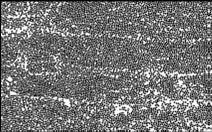
Figure 1: Fiber-reinforced composite.

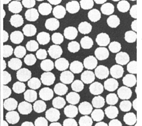
Figure 2: Microstructure.

In general it is impossible to record the relative location of every fiber for an entire structure made from a composite material. Hence some stochastic information needs to be extracted from the structure and used to describe the coefficient matrix. An investigation of the different stochastic data that can be obtained from composite samples is taken up in [2]. As mentioned earlier we will assume that the problem is deterministic with well defined coefficients. Future work will address the problem of determination of the approximation error for stochastically defined coefficients.

2 The generalized finite element method (GFEM)

The GFEM is based on the partition of unity method (PUM) and is introduced in [5] as a method for the numerical solution of elliptic PDE with rough coefficients. The method is further elaborated and extended to other application areas in the works of [3], [4], [24] and [25]. We briefly summarize the main ideas and results of GFEM. For more details see [3]. We recall the scalar Dirichlet and Neumann boundary value problems defined in section 1.1. For the Dirichlet problem define the hyperplane $H_{q}^{1}(\Omega)=\{u\in H^{1}(\Omega)\mid u=q(x)$ on $\partial\Omega\}$ and set $H_{0}^{1}(\Omega)=H_{q}^{1}(\Omega)$ for $q=0$. The weak solution of the Dirichlet problem $u_{0}\in H_{q}^{1}(\Omega)$ satisfies

$$B(u_{0},v)=F(v),$$ (2.1)

for all $v\in H_{0}^{1}(\Omega)$ where

$$B(u,v)=\int_{\Omega}A(x)\nabla u\cdot\nabla v\,dx, F(v)=\int_{\Omega}f\,vdx.$$ and (2.2)

For the Neumann boundary value problem the solution $u_{0}\in H^{1}(\Omega)$ satisfies (2.1) for all $v\in H^{1}(\Omega)$ and

$$F(v)=\int_{\Omega}fvdx+\int_{\partial\Omega}gvds$$

For future reference we note that the energy norm (1.6) is given by $\parallel u\parallel_{\mathcal{E}(\Omega)}=(B(u,u))^{1/2}$.

We now recall that for a $N$ dimensional space $S(\Omega)\subset H^{1}(\Omega)$ that the associated Galerkin solution of the Neumann problem  $u^{S}\in S(\Omega)\subset H^{1}(\Omega)$ satisfies $B(u^{S},v)=F(v)$ for all $v\in S(\Omega)$. For a fixed tolerance $\varepsilon>0$ if there is a $\psi\in S(\Omega)$ such that $\parallel u_{0}-\psi\parallel_{\scriptscriptstyle{\mathcal{E}(\Omega)}}\leq\varepsilon$ then it is clear that the Galerkin solution satisfies $\parallel u_{0}-u^{S}\parallel_{\scriptscriptstyle{\mathcal{E}(\Omega)}}\leq\varepsilon$. A similar conclusion holds for the Galerkin solution of the Dirichlet problem. Let $S_{0}(\Omega)$ be an $N$ dimensional subspace of $H_{0}^{1}(\Omega)$ and set $S_{q}(\Omega)=S_{0}(\Omega)\oplus\Phi_{0}$ where $\Phi_{0}$ is a particular function belonging to $H_{q}^{1}$($\Omega)$. Then the Galerkin solution of the Dirichlet problem $u^{S}\in S_{q}(\Omega)$ satisfies $B(u^{S},v)=F(v)$ for $\forall v\in S_{0}(\Omega).$ Again it is clear that if there exists a $\psi\in S_{q}(\Omega)$ such that $\parallel u_{0}-\psi\parallel_{\scriptscriptstyle{\mathcal{E}(\Omega)}}\leq\varepsilon$ then $\parallel u_{0}-u^{S}\parallel_{\scriptscriptstyle{\mathcal{E}(\Omega)}}\leq\varepsilon$. Hence the main task in constructing a Galerkin numerical solution is the selection of $S(\Omega)$ for the Neumann problem and the selection of the hyperplane $S_{q}(\Omega)$ for the Dirichlet problem.

We introduce the Galerkin approximation delivered by GFEM and discuss the associated approximation error. Since most physical situations are described by Neumann boundary conditions we address this case and note that the Dirichlet case follows identical lines. Let $\{\mathcal{O}_{i}\}_{i=1}^{m}$, be a collection of open sets that cover the computational domain, i.e., $\Omega\subset\cup_{i=1}^{m}\mathcal{O}_{i}$, and we introduce the partition of unity subordinate to the open cover denoted by $\phi_{i}\in C^{1}(\mathcal{O}_{i})$, $i=1,...m$. We relabel interior sets $\mathcal{O}_{i}\subset\Omega$ as $\omega_{i}=\mathcal{O}_{i}$ and for sets $\mathcal{O}_{i}$ that intersect the boundary of $\Omega$ we write $\omega_{i}=\mathcal{O}_{i}\cap\Omega$. Here $\cup_{i=1}^{m}\omega_{i}=\Omega$ and we assume that each point $x\in\Omega$ belongs to at most $\kappa$ subdomains $\omega_{i}$. The functions $\phi_{i}$, $i=1,\ldots,m$ have the following properties

$$0\leq\phi_{i}\leq 1, i=1,\ldots,m,$$ (2.3)

$$\phi_{i}(x)=0, x\in\Omega\backslash\omega_{i}, i=1,..m$$ for (2.4)

$$\sum_{i=1}^{m}\phi_{i}(x)=1, \hbox{ $\forall x\in\Omega$},$$ (2.5)

$$\max_{x\in\Omega}\mid\phi_{i}(x)\mid \leq C_{1},\,\,\,\,i=1,...m$$ (2.6)

$$\max_{x\in\Omega}\mid\nabla\phi_{i}(x)\mid \leq \frac{C_{2}}{diam(\omega_{i})},\,\,\,\,i=1,...m,$$ (2.7)

where the constants $C_{1}$ and $C_{2}$ are positive and bounded. Here $diam(\omega_{i})$ denotes the diameter of $\omega_{i}.$

Next we introduce local approximation spaces associated with each $\omega_{i}$. For this case let $\Psi_{i}$ be a finite dimensional subspace of $H^{1}(\omega_{i})$ of dimension $N_{i}$. The trial and test spaces for the GFEM are constructed from the local approximation spaces and are defined by

$$S(\Omega)=\left\{\psi;\,\psi=\sum_{i=1}^{m}\sum_{j=1}^{N_{i}}\phi_{i}\xi_{i}^{[j]},\hbox{ where }\xi_{i}^{[j]}\in\Psi_{i},\,\right\}.$$ (2.8)

Note that although $\xi_{i}^{[j]}$ only belongs to $H^{1}(\omega_{i})$ the PUM construction ensures that $S(\Omega)\subset H^{1}(\Omega)$. Here the dimension $N$ of $S(\Omega)$ is given by $N=\sum_{i=1}^{m}N_{i}$.

An analogous approach using local approximation spaces is used for the Dirichlet problem. Here the only difference is when $\overline{\omega}_{j}\cap\partial\Omega\neq 0$. For this case if $q=0$ then $\Psi_{j}\subset H^{1}(\omega_{j})\cap H_{0}^{1}(\Omega)$ and if $q\neq 0$ then $\Psi_{j}\subset(H^{1}(\omega_{j})\cap H_{0}^{1}(\Omega))\oplus\Phi_{j}$ where $\Phi_{j}$ is a particular function belonging to $H^{1}(\omega_{j})\cap H_{q}^{1}(\Omega)$.

It is now clear from the formulation that the approximation error of the Galerkin numerical solution for the GFEM is tied to the accuracy of the local approximation spaces. With this in mind we state the following approximation theorem [4] for the Neumann problem.

Theorem 2.1.

Suppose that there exists $\zeta_{i}\in\Psi_{i}$, $i=1,\ldots,m$ with

$$\parallel u_{0}-\zeta_{i}\parallel_{L^{2}_{\ast}(\omega_{i})} = (\int_{\omega_{i}}\beta^{\ast}(u_{0}-\zeta_{i})^{2}dx)^{1/2}\leq\varepsilon_{1}(i)$$ (2.9)

$$\parallel u_{0}-\zeta_{i}\parallel_{\mathcal{E}(\omega_{i})} \leq \varepsilon_{2}(i)$$ (2.10)

and let

$$\zeta(x)=\sum_{i=1}^{m}\zeta_{i}(x)\phi_{i}(x)$$

then $\zeta(x)\in H^{1}(\Omega)$ and

$$\parallel u_{0}-\zeta\parallel_{L^{2}_{\ast}(\Omega)} \leq C_{1}(\sum_{i=1}^{m}(\varepsilon_{1}(i))^{2})^{1/2}$$ (2.11)

$$\parallel u_{0}-\zeta\parallel_{\mathcal{E}(\Omega)} \leq (C_{2}^{2}\sum_{i=1}^{m}(\varepsilon_{1}^{2}(i)/diam^{2}(\omega_{i}))+C_{1}^{2}\sum_{i=1}^{m}\varepsilon_{2}^{2}(i))^{1/2},$$ (2.12)

where $C_{1}$ and $C_{2}$ are as in (2.6) and (2.7) respectively.

Moreover if all local spaces $\Psi_{i}$ contain the subspace of constant functions then, for an appropriate choice of constant, the first term on the right hand side of (2.12) can be omitted as it is majorized by the second term.

We remark that Theorem 2.1 also holds true for Dirichlet boundary conditions. For this case the only modifications are the ones previously discussed for the subdomains $\omega_{j}$ that intersect the boundary. Theorem 2.1 shows that the proper selection of the local approximation spaces $\Psi_{i}$ are essential for obtaining optimal accuracy. In the next section we identify local spaces $\Psi_{i}$ that deliver a nearly exponential rate of convergence with respect to the dimension of the trial space.

3 Optimal local approximation spaces and nearly exponential upper bounds on their accuracy

We identify the optimal local approximation spaces for GFEM and provide an upper bound on the accuracy of their approximation. We will consider the case when the exact solution $u_{0}$ solves the Neumann problem with $f=0$ in (1.1). During the course of the exposition we will indicate the modifications needed to treat the corresponding Dirichlet problem. The generalization to the case $f\neq 0$ will be addressed as part of the implementation given in section 4.

We recall the local approximation spaces introduced in section 2 denoted by $\Psi_{i}$ defined on the sets $\omega_{i}$. To fix ideas we will assume that $\omega_{i}$ are the cubes of a given side length surrounded by a larger cube $\omega_{i}^{\ast}$. We will distinguish two cases depending on if the set $\omega_{i},$ lies within the interior of $\Omega$ or if $\overline{\omega}_{i}\cap\partial\Omega\not=\emptyset$. It will be shown that the overall approach to constructing optimal local approximation spaces for these two cases is the same. We drop subscripts and consider concentric cubes $\omega\subset\omega^{\ast}$ with side lengths given by $\sigma$ and $\sigma^{*}=(1+\rho)\sigma$ respectively. In order to introduce the ideas we suppose first that $\omega$ lies in the interior of $\Omega$ so that $\omega\subset\omega^{*}\subset\Omega$. The energy inner products associated with these subsets are defined by

$$(u,v)_{\mathcal{E}(\omega)}=\int_{\omega}A\nabla u\cdot\nabla v\,dx (u,v)_{\mathcal{E}(\omega^{*})}=\int_{\omega^{*}}A\nabla u\cdot\nabla v\,dx.$$ (3.1)

We shall utilize $\omega^{*}$ to construct a finite dimensional approximation space over $\omega$. For any open subset $S$ of the computational domain $\Omega$ we introduce the space of functions $H_{A}(S)$ defined to be the functions in $H^{1}(S)$ that are $A$-harmonic on $S$, i.e., $v\in H^{1}(S)$ and

$$B(v,\varphi)=0,\,\,\,\,\forall\varphi\in C_{0}^{\infty}(S).$$

Here $H_{A}(\omega)$ and $H_{A}(\omega^{*})$ contain local information on the heterogeneities and will be used in the construction of the optimal local basis. We introduce the quotient of $H_{A}(\omega^{*})$ with respect to the constant functions denoted by $H_{A}(\omega^{*})/\mathbb{R}$. It is clear that the solution $u_{0}$ lies in this local space modulo a constant.

In this method we choose to approximate elements in the space of functions $H_{A}(\omega^{*})/\mathbb{R}$ restricted to $\omega$. This choice is motivated by the Caccioppoli inequality (3.11), proved in Appendex A, which is used to estimate the energy norm over $\omega$ in terms of the $L^{2}$ norm over $\omega^{*}$. Let $P:H_{A}(\omega^{*})/\mathbb{R}\rightarrow H_{A}(\omega)/\mathbb{R}$ be the restriction operator such that $P(u)(x)=u(x)$ for all $x\in\omega$ and $u\in H_{A}(\omega^{*})/\mathbb{R}$. The operator $P$ is compact, this follows from the Caccioppoli inequality, and the compactness proof is given in the Appendix, see Theorem A.1.

Now we approximate by “$n$” dimensional subspaces $S(n)\subset H_{A}^{1}(\omega)/\mathbb{R}$. The accuracy of a particular increasing sequence $\left\{S(n)\right\}_{n=1}^{\infty}$ of local approximation spaces is measured by

$$d(S(n),\omega)=\sup_{u\in H_{A}(\omega^{*})/\mathbb{R}}\inf_{\chi\in S(n)}\frac{\|Pu-\chi\|_{\mathcal{E}(\omega)}}{\|u\|_{\mathcal{E}(\omega^{*})}}.$$ (3.2)

A sequence of approximation spaces $\hat{S}(n)$ is said to be optimal if it has an accuracy $d(\hat{S}(n),\omega)$ that satisfies $d(\hat{S}(n),\omega)\leq d(S(n),\omega)$, $n=1,2,\ldots$, when compared to any other sequence of approximation spaces $S(n)$. The problem of finding the family of optimal local approximation spaces is formulated as follows. Let

$$d_{n}(\omega,\omega^{*})=\inf_{S(n)}\sup_{u\in H_{A}(\omega^{*})/\mathbb{R}}\inf_{\chi\in S(n)}\frac{\|Pu-\chi\|_{\mathcal{E}(\omega)}}{\|u\|_{\mathcal{E}(\omega^{*})}}.$$ (3.3)

Then the optimal family of approximation spaces $\{\Psi_{n}(\omega)\}_{n=1}^{\infty}$ satisfy

$$d_{n}(\omega,\omega^{*})=\sup_{u\in H_{A}(\omega^{*})/\mathbb{R}}\inf_{\chi\in\Psi_{n}(\omega)}\frac{\|Pu-\chi\|_{\mathcal{E}(\omega)}}{\|u\|_{\mathcal{E}(\omega^{*})}}.$$ (3.4)

The quantity $d_{n}(\omega,\omega^{*})$ is known as the Kolomogorov n-width of the compact operator $P$ see, [22].

The optimal local approximation space $\Psi_{n}(\omega)$ for GFEM follows from general considerations. We introduce the adjoint operator $P^{*}:H_{A}(\omega)/\mathbb{R}\rightarrow H_{A}(\omega^{*})/\mathbb{R}$ and the operator $P^{*}P$ is a compact, self adjoint, non-negative operator mapping $H_{A}(\omega^{*})/\mathbb{R}$ into itself. We denote the eigenfunctions and eigenvalues of the problem

$$P^{*}Pu=\lambda u$$ (3.5)

by $\{\varphi_{i}\}$ and $\{\lambda_{i}\}$ and apply Theorem 2.2, Chapter 4 of [22] to see that the optimal subspace $\Psi_{n}$ is given by the following theorem.

Theorem 3.1.

The optimal approximation space is given by $\Psi_{n}(\omega)=span\{\psi_{1},\ldots,\psi_{n}\}$, where $\psi_{i}=P\varphi_{i}$ and $d_{n}(\omega,\omega^{*})=\sqrt{\lambda_{n+1}}$.

For the case considered here the definitions of $P$ and $P^{*}$ show that the optimal subspace and eigenvalues are given by the following explicit eigenvalue problem.

Theorem 3.2.

The optimal approximation space is given by $\Psi_{n}(\omega)=span\{\psi_{1},\ldots,\psi_{n}\}$ where $\psi_{i}=P\varphi_{i}$ and $\varphi_{i}$ and $\lambda_{i}$ are the first $n$ eigenfunctions and eigenvalues that satisfy

$$(\varphi_{i},\delta)_{\scriptscriptstyle{\mathcal{E}(\omega)}} = \lambda_{i}(\varphi_{i},\delta)_{\scriptscriptstyle{\mathcal{E}(\omega^{*})}}\hbox{, $\forall\delta\in H_{A}(\omega^{*})/\mathbb{R}$}.$$ (3.6)

Proof. The eigenvalue problem (3.5) is given by

$$(P^{*}Pu,\delta)_{\scriptscriptstyle{\mathcal{E}(\omega^{*})}} = \lambda(u,\delta)_{\scriptscriptstyle{\mathcal{E}(\omega^{*})}}\hbox{, $\forall\delta\in H_{A}(\omega^{*})/\mathbb{R}$}.$$ (3.7)

The theorem follows from (3.7) noting that

$$(P^{*}Pu,\delta)_{\scriptscriptstyle{\mathcal{E}(\omega^{*})}}=(Pu,P\delta)_{\scriptscriptstyle{\mathcal{E}(\omega)}}=(u,\delta)_{\scriptscriptstyle{\mathcal{E}(\omega)}}.$$ (3.8)

The next theorem provides an upper bound on the rate of convergence for the optimal local approximation.

Theorem 3.3.

Exponential convergence for interior approximations.

For $\epsilon>0$ there is an $N_{\epsilon}>0$ such that for all $n>N_{\epsilon}$

$$d_{n}(\omega,\omega^{*})\leq e^{-n^{\left(\frac{1}{d+1}-\epsilon\right)}}.$$ (3.9)

The index $N_{\epsilon}$ is constructed explicitly in the proof of Theorem 3.3 given in the next section. Theorem 3.3 shows that the asymptotic convergence rate associated with the optimal approximation space is nearly exponential for the general class of $L^{\infty}(\Omega)$ coefficients belonging to $\mathfrak{C}$. In section 3.2 we identify the optimal local approximation space for the case when $\omega$ touches the boundary of the computational domain. In that section we show that the convergence rate is also nearly exponential with respect to the degrees of freedom of the optimal local approximation space. We collect our results in section 3.3 and recall Theorem 2.1 to obtain the nearly exponential convergence rate for GFEM stated in Theorem 3.10.

3.1 Local approximation on the interior

In this section we establish Theorem 3.3. To do this we construct a family of approximation spaces that exhibit nearly exponential convergence in the accuracy of approximation. The convergence rate for this family delivers an upper bound on the convergence rate for the optimal local approximation space described by Theorem 3.2.

For future reference we introduce the decomposition of $H^{1}(\omega^{*})$ given by

$$H^{1}(\omega^{*})=H_{A}^{0}(\omega^{*})+H_{0}^{1}(\omega^{*})+\mathbb{R}.$$

Here $H_{A}^{0}(\omega^{*})$ is the subspace of $H_{A}(\omega^{*})$ given by the functions with zero average over $\omega^{*}$. The spaces $H_{A}^{0}(\omega^{*})$ and $H_{0}^{1}(\omega^{*})$ are orthogonal with respect to the energy inner product $(\cdot,\cdot)_{\mathcal{E}(\omega^{*})}$. The orthogonal projection from $H^{1}(\omega^{*})$ onto $H_{A}^{0}(\omega^{*})$ is denoted by $\mathcal{P}^{A}$.

The construction of the local approximation space is done iteratively. We start by introducing the the first $n$ non-constant eigenfunctions $v_{i}\in H^{1}(\omega^{*})$ of the Neumann eigenvalue problem

$$(v_{i},w)_{\mathcal{E}(\omega^{*})}=\lambda_{i}\int_{\omega^{*}}v_{i}w\,dx,\hbox{ $\forall$ $w\in H^{1}(\omega^{*})$}$$

posed over $\omega^{\ast}$, $i=1,\ldots,n$. The subspace spanned by these functions is denoted by $S_{n}(\omega^{*})$. Next we introduce the span of $A$ harmonic functions given by

$$W_{n}(\omega^{\ast})=\hbox{span}\{w_{i}\in H_{A}^{0}(\omega^{\ast}):\,w_{i}=v_{i},\hbox{ on }\partial\omega^{\ast},\,i=1,\ldots n\}$$ (3.10)

One readily checks that $W_{n}(\omega^{*})=\mathcal{P}^{A}S_{n}(\omega^{*})$.

We define the family of approximation spaces $\mathcal{F}_{n}(\omega,\omega^{\ast})$ given by the restriction of the elements of $W_{n}(\omega^{\ast})$ to $\omega$. In what follows we first show that $\mathcal{F}_{n}(\omega,\omega^{\ast})$ is a family of local approximation spaces with a rate of convergence on the order of $n^{-1/d}$, for $d=2,3$. To show this we introduce a suitable version of the Cacciappoli inequality that bounds functions in the energy norm over any measurable subset $\mathcal{O}\subset\omega^{\ast}$ for which $dist(\partial\mathcal{O},\partial\omega^{\ast})>\delta>0$ in terms of the $L^{2}$ norm over $\omega^{\ast}$.

Lemma 3.1.

Let $u$ be $A$-harmonic in $\omega^{\ast}$ and belong to $L^{2}(\omega^{\ast})\cap H_{loc}^{1}(\omega^{\ast})$. Then

$$\parallel u\parallel_{\mathcal{E}(\mathcal{O})}\leq(2(\beta)^{1/2}/\delta)\parallel u\parallel_{L^{2}(\omega^{\ast})}.$$ (3.11)

where $\beta$ is defined in (1.5).

The proof of Lemma 3.1 is given in the Appendix. Next we introduce the approximation theorem associated with the space $W_{n}(\omega^{*})$ given by

Lemma 3.2.

Let $u\in H_{A}^{0}(\omega^{\ast})$ then there exists a $v_{u}\in W_{n}(\omega^{*})$ such that

$$\|u-v_{u}\|_{L^{2}(\omega^{*})}=\inf_{v\in W_{n}(\omega^{\ast})}\parallel u-v\parallel_{L^{2}(\omega^{\ast})}\leq C_{n}\sigma^{\ast}\frac{\gamma_{d}^{1/d}}{\sqrt{4\pi}}\alpha^{-1/2}\parallel u\parallel_{\mathcal{E}(\omega^{\ast})}$$ (3.12)

where $\sigma^{\ast}$   is the side length of the cube $\omega^{\ast},$ $\gamma_{d}$ is the volume of the unit ball in $\mathbb{R}^{d}$ and $C_{n}=n^{-1/d}(1+o(1))$, for $d=2,3$.

Proof. The lemma follows immediately from an upper bound on the quotient

$$R=\sup_{u\in H_{A}^{0}(\omega^{\ast})}\inf_{w\in W_{n}(\omega^{\ast})}\frac{\|u-w\|_{L^{2}(\omega^{\ast})}}{\|u\|_{\mathcal{E}(\omega^{\ast})}}.$$ (3.13)

Fix $u\in H_{A}(\omega^{\ast})^{0}$ and denote the projection of $u$ onto $W_{n}(\omega^{\ast})$ with respect to the energy norm $\|\cdot\|_{\mathcal{E}(\omega^{\ast})}$ by $\mathcal{P}^{\mathcal{E}}u$. Choosing $w=\mathcal{P}^{\mathcal{E}}u$ and noting that $\|(I-\mathcal{P}^{\mathcal{E}})u\|_{\mathcal{E}(\omega^{\ast})}\leq\|u\|_{\mathcal{E}(\omega^{\ast})}$ gives the upper bound

$$R\leq\sup_{u\in H_{A}^{0}(\omega^{\ast})\perp\,W_{n}(\omega^{\ast})}\frac{\|u\|_{L^{2}(\omega^{\ast})}}{\|u\|_{\mathcal{E}(\omega^{\ast})}}.$$ (3.14)

Since $W_{n}(\omega^{\ast})=\mathcal{P}^{A}S_{n}(\omega^{\ast})$ it follows that

$$\{u\in H_{A}^{0}(\omega^{*})\perp\mathcal{P}^{A}S_{n}(\omega^{*})\}=\{u\in H_{A}^{0}(\omega^{*})\perp S_{n}(\omega^{*})\},$$

$$\{u\in H_{A}^{0}(\omega^{*})\perp S_{n}(\omega^{*})\}\subset\{u\in H^{1}(\omega^{*})\perp(S_{n}(\omega^{*})+\mathbb{R})\},$$ (3.15)

where the $\perp$ in the second line of (3.15) is with respect to the $L^{2}(\omega^{*})$ inner product. Hence

$$R\leq\sup_{u\in H_{A}^{0}(\omega^{\ast})\perp\,S_{n}(\omega^{\ast})}\frac{\|u\|_{L^{2}(\omega^{\ast})}}{\|u\|_{\mathcal{E}(\omega^{\ast})}}\leq\sup_{u\in H^{1}(\omega^{\ast})\perp\,(S_{n}(\omega^{\ast})+\mathbb{R})}\frac{\|u\|_{L^{2}(\omega^{\ast})}}{\|u\|_{\mathcal{E}(\omega^{\ast})}}=\frac{1}{\sqrt{\mu_{n+1}}},$$ (3.16)

where $\mu_{n+1}$ is the largest Neumann eigenvalue associated with $S_{n+1}(\omega^{\ast})$. One has the elementary lower bound $\mu_{n+1}\geq\alpha\nu_{n+1}$ where $\nu_{n+1}=4\pi C_{n}^{-2}(\sigma^{*}\gamma_{d}^{1/d})^{-2}$ is the corresponding Neumann eigenvalue for the Laplacian with on squares ($d=2$) or cubes ($d=3$). The required upper bound on $R$ now follows and the theorem is proved.

Now we apply Theorem 3.1 to $u-v_{u}$ on $\omega\subset\omega^{\ast}$ and combine it with Theorem 3.2 to obtain the following convergence rate associated with the family of approximation spaces $\mathcal{F}_{n}(\omega,\omega^{\ast})$ given by

Theorem 3.4.

Let $u\in{H}_{A}^{0}(\omega^{\ast})$ then there exists an approximation $v_{u}\in\mathcal{F}_{n}(\omega,\omega^{\ast})$ for which

$$\parallel u-v_{u}\parallel_{\mathcal{E}(\omega)}\,=\inf_{v\in\mathcal{F}_{n}(\omega,\omega^{\ast})}\parallel u-v\parallel_{\mathcal{E}(\omega)}\,\leq I(\omega,\omega^{\ast})\,C_{n}\parallel u\parallel_{\mathcal{E}(\omega^{\ast})}$$ (3.17)

where

$$I(\omega,\omega^{\ast})=2\,\frac{\gamma_{d}^{1/d}}{\sqrt{\pi}}\,\frac{1+\rho}{\rho}(\beta/\alpha)^{1/2} C_{n}=n^{-1/d}(1+o(1)),\,\,d=2,3,$$ and (3.18)

where $\gamma_{d}$ is the volume of the unit ball in dimension $d$.

Next we proceed iteratively to construct a family of local approximation spaces with a rate of convergence that is nearly exponential. For any pair of two concentric cubes $Q\subset Q^{\ast}$ we define $\mathcal{F}_{n}(Q,Q^{\ast})$ to be the space given by the restriction of $W_{n}(Q^{\ast})$ on $Q$. We suppose that $\omega^{\ast}$ is of side length $\sigma^{*}$. Let $N>1$ be an integer and we suppose that $\omega$ is of side length $\sigma$ and $\sigma^{*}=\sigma(1+\rho)$. Choose $\omega_{j}$, $j=1,2,...N$ to be the nested family of concentric cubes with side length $\frac{\sigma}{2}(1+\rho(N+1-j)/N)$ for which $\omega=\omega_{N+1}\subset\omega_{N}\subset\omega_{N-1}\subset\cdots\subset\omega_{1}=\omega^{\ast}$. We introduce the local spaces, $\mathcal{F}_{n}(\omega,\omega_{N})$, $\mathcal{F}_{n}(\omega,\omega_{N-1})$,…,$\mathcal{F}_{n}(\omega,\omega_{1})$. Put $m=N\times n$ and we define the approximation space given by

$$\mathcal{T}(m,\omega,\omega^{\ast})=\mathcal{F}_{n}(\omega,\omega_{1})+\cdots+\mathcal{F}_{n}(\omega,\omega_{N}).$$ (3.19)

The convergence rate associated with the local approximation space $\mathcal{T}(m,\omega,\omega^{\ast})$ is given in the following theorem.

Theorem 3.5.

Let $u\in{H}_{A}^{0}(\omega^{\ast})$ and $N\geq 1$ be an integer. Then there exists $z_{u}\in\mathcal{T}(m,\omega,\omega^{\ast})$ such that

$$\parallel u-z_{u}\parallel_{\mathcal{E(\omega)}}\leq\varsigma^{N}\parallel u\parallel_{\mathcal{E}(\omega^{\ast})}$$ (3.20)

and $\varsigma=2\,\frac{\gamma_{d}^{1/d}}{\sqrt{\pi}}\,\frac{1+\rho}{\rho}\,N(\beta/\alpha)^{1/2}C_{n}$.

Proof. In what follows we make the identification $\omega_{0}=\omega^{*}$ and $\omega_{N+1}=\omega$. From Theorem 3.4 we have that there exists $v_{1}\in\mathcal{F}_{n}(\omega_{1},\omega^{\ast})$ such that

$$\|u-v_{1}\|_{\mathcal{E}(\omega_{1})}\leq\varsigma\parallel u\parallel_{\mathcal{E}(\omega^{\ast})}$$ (3.21)

Suppose next that for $m=1,\ldots,j$ there are functions $v_{m}\in\mathcal{F}_{n}(\omega_{m},\omega_{m-1})$ such that

$$\parallel u-\sum_{m=1}^{j}v_{m}\parallel_{\mathcal{E}(\omega_{j})}\leq\varsigma^{j}\parallel u\parallel_{\mathcal{E}(\omega^{\ast})}$$ (3.22)

Applying Theorem 3.4 we see that there exists a $v_{j+1}\in\mathcal{F}_{n}(\omega_{j+1},\omega_{j})$ for which

$$\|u-(\sum_{m=1}^{j}v_{m})-v_{j+1}\|_{\mathcal{E}(\omega_{j+1})}\leq\varsigma\parallel u-\sum_{m=1}^{j}v_{m}\parallel_{\mathcal{E}(\omega_{j})}$$ (3.23)

and the induction step goes through. Choosing $z_{u}=\sum_{m=1}^{N}v_{m}$ delivers

$$\parallel u-z_{u}\parallel_{\mathcal{E(\omega)}}\leq\varsigma^{N}\parallel u\parallel_{\mathcal{E(\omega}^{\ast})}$$ (3.24)

and the theorem follows noting that $z_{u}$ belongs to $\mathcal{T}(m,\omega,\omega^{\ast})$.

Next we make a choice for $N$. We choose $N$ to be the largest integer less than or equal to $n^{\gamma}$ for $0<\gamma$. Thus $m\leq n^{\gamma+1}$ and $m^{\frac{1}{\gamma+1}}\leq n$ and it follows that $n^{-\frac{1}{d}}\leq m^{-\frac{1}{d(\gamma+1)}}$, and $N\leq m^{\frac{\gamma}{\gamma+1}}$. On applying these inequalities we obtain

$$\varsigma^{N}\leq\exp{\left\{-m^{\frac{\gamma}{\gamma+1}}\left(-\ln{K}+\frac{1/d-\gamma}{\gamma+1}\ln{m}\right)\right\}}$$ (3.25)

where $K=2\,\frac{\gamma_{d}^{1/d}}{\sqrt{\pi}}(\frac{\beta}{\alpha})^{1/2}(\frac{1+\rho}{\rho})$. It is evident that decay occurs for the choice $0\leq\gamma<\frac{1}{d}$ and

$$\varsigma^{N}<e^{-m^{\frac{\gamma}{\gamma+1}}}$$ (3.26)

for $m>N=(Ke)^{(\gamma+1)/(1/d-\gamma)}$. We set $\ell={\rm dimension}\{\mathcal{T}(m,\omega,\omega^{\ast})\}$ and Theorem 3.5 together with (3.26) imply

$$d_{\ell}(\omega,\omega^{*})\leq\sup_{u\in H_{A}(\omega^{*})/\mathbb{R}}\inf_{\chi\in\mathcal{T}(m,\omega,\omega^{\ast})}\frac{\|u-\chi\|_{\mathcal{E}(\omega)}}{\|u\|_{\mathcal{E}(\omega^{*})}}\leq e^{-\ell^{\frac{\gamma}{\gamma+1}}}.$$ (3.27)

for $\ell>N$ and Theorem 3.3 is proved.

3.2 Local approximation at the boundary

Consider two concentric cubes $C\subset\omega^{*}$ of side lengths $\sigma$ and $\sigma^{*}=(1+\rho)\sigma$ respectively. We suppose that $\omega^{*}\cap\Omega\not=\emptyset$ and $\omega^{*}\cap\partial\Omega\not=\emptyset$. The truncated cube $\omega$ is defined to be $\omega=C\cap\Omega$, and $\partial\omega\cap\partial\Omega\not=\emptyset$, see Figure 3. For this case we will assume that $\partial\Omega$ is $C^{1}$, i.e., the boundary can be represented locally as the graph of a $C^{1}$ function. The method presented here applies to both Dirichlet and Neumann boundary value problems. We will illustrate the ideas for the Neumann problem and make references to the Dirichlet problem when appropriate. Given a function $u\in H_{A}(\Omega)$ the goal is to provide a local approximation to $u$ in $\omega$. To this end we form a local particular solution $u_{p}$ given by the $A$-harmonic function that satisfies $n\cdot A\nabla u_{p}=g$ on $\omega^{*}\cap\partial\Omega$ and $u_{p}=0$ on $\partial\omega^{*}\cap\Omega$. Writing $u=u_{p}+u_{0}$ we see that $n\cdot A\nabla u_{0}=0$ on $\omega^{*}\cap\partial\Omega$ and $u_{0}=u$ on $\partial\omega^{*}\cap\Omega$. If instead we have Dirichlet data then the particular solution $u_{p}$ satisfies $u_{p}=q=u$ on $\omega^{*}\cap\partial\Omega$ and $u_{p}=0$ on $\partial\omega^{*}\cap\Omega$. The objective of this section is to find the optimal family of local approximation spaces that give the best approximation to $u_{0}=u-u_{p}$ in the energy norm over the set $\omega$. To this end we introduce the the space of functions $H_{A,0}(\Omega\cap\omega^{\ast})$ given by all functions $v$ in $H^{1}(\Omega\cap\omega^{\ast})$ that are $A$-harmonic on $\Omega\cap\omega^{\ast}$ and for which

$$\partial_{\nu}v\equiv n\cdot A\nabla v=0$$

on $\partial\Omega\cap\omega^{\ast}$. The analogous space of functions defined on $\omega$ is denoted by $H_{A,0}(\omega)$. Since we approximate functions with respect to the energy norm we introduce the quotient space of $H_{A,0}(\Omega\cap\omega^{\ast})$ with respect to the constant functions denoted by $H_{A,0}(\Omega\cap\omega^{\ast})/\mathbb{R}$.

Now we introduce $P:H_{A,0}(\omega^{*}\cap\Omega)/\mathbb{R}\rightarrow H_{A,0}(\omega)/\mathbb{R}$ given by the restriction operator defined by $P(u)(x)=u(x)$ for all $x\in\omega$ and $u\in H_{A,0}(\omega^{*}\cap\Omega)/\mathbb{R}$. The operator $P$ is compact, this follows from Lemma A.2 given in the Appendix. Let $S(n)$ be any finite dimensional subspace of $H_{A,0}(\omega)/\mathbb{R}$ and the problem of finding the family of optimal local approximation spaces is formulated in terms of the n-width of $P$. Let

$$d_{n}(\omega,\omega^{*}\cap\Omega)=\inf_{S(n)}\sup_{u\in H_{A,0}(\omega^{*}\cap\Omega)/\mathbb{R}}\inf_{\chi\in S(n)}\frac{\|Pu-\chi\|_{\mathcal{E}(\omega)}}{\|u\|_{\mathcal{E}(\omega^{*}\cap\Omega)}}.$$ (3.28)

Then the optimal family of boundary approximation spaces $\{\Psi_{n}(\omega)\}_{n=1}^{\infty}$ for GFEM satisfy

$$d_{n}(\omega,\omega^{*}\cap\Omega)=\sup_{u\in H_{A,0}(\omega^{*}\cap\Omega)/\mathbb{R}}\inf_{\chi\in\Psi_{n}(\omega)}\frac{\|Pu-\chi\|_{\mathcal{E}(\omega)}}{\|u\|_{\mathcal{E}(\omega^{*}\cap\Omega)}}.$$ (3.29)

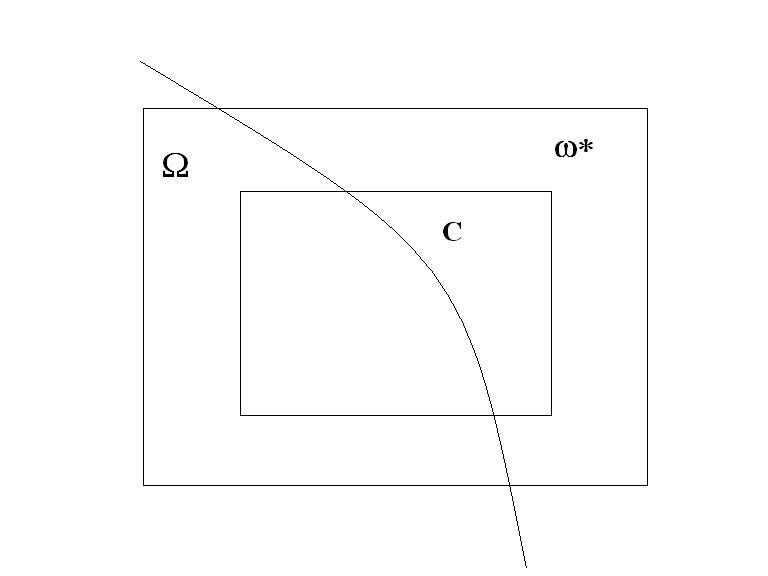
Figure 3: Truncated cube $\omega=C\cap\Omega$.

Proceeding as before we introduce the adjoint operator $P^{*}:H_{A}(\omega)/\mathbb{R}\rightarrow H_{A}(\omega^{*}\cap\Omega)/\mathbb{R}$ and the operator $P^{*}P$ is a compact operator mapping $H_{A,0}(\omega^{*}\cap\Omega)/\mathbb{R}$ into itself. Similar arguments show that the optimal approximating spaces are given by the following theorem.

Theorem 3.6.

The optimal approximation space is given by $\Psi_{n}(\omega)=span\{\psi_{1},\ldots,\psi_{n}\}$ where $\psi_{i}=P\varphi_{i}$ and $\varphi_{i}\in H_{A,0}(\omega^{*}\cap\Omega)/\mathbb{R}$ and $\lambda_{i}$ are the first $n$ eigenfunctions and eigenvalues that satisfy

$$(\varphi_{i},\delta)_{\scriptscriptstyle{\mathcal{E}(\omega)}} = \lambda_{i}(\varphi_{i},\delta)_{\scriptscriptstyle{\mathcal{E}(\omega^{*}\cap\Omega)}}\hbox{, $\forall\delta\in H_{A,0}(\omega^{*}\cap\Omega)/\mathbb{R}$}.$$ (3.30)

The next theorem provides an upper bound on the rate of convergence for the optimal local boundary approximation.

Theorem 3.7.

Exponential convergence at the boundary.

For $\epsilon>0$ there is an $N_{\epsilon}>0$ such that for all $n>N_{\epsilon}$

$$d_{n}(\omega,\omega^{*}\cap\Omega)\leq e^{-n^{\left(\frac{1}{d+1}-\epsilon\right)}}.$$ (3.31)

Theorem 3.7 shows that the asymptotic convergence rate associated with the optimal boundary approximation space is also nearly exponential for the general class of $L^{\infty}(\omega^{*})$ coefficients $\mathfrak{C}$.

We now give the prof of Theorem 3.7. The subspace of A-harmonic functions defined over $\Omega\cap\omega^{*}$ with zero mean is denoted by $H_{A}^{0}(\Omega\cap\omega^{*})$ and the subspace of elements belonging to $H_{A,0}(\Omega\cap\omega^{\ast})$ with zero mean over $\Omega\cap\omega^{*}$ is denoted by $H_{A,0}^{0}(\Omega\cap\omega^{\ast})$. We introduce the $L^{2}(\Omega\cap\omega^{\ast})$ norm closure of $H_{A,0}^{0}(\Omega\cap\omega^{\ast})$ denoted by $\overline{H}_{A,0}^{0}(\Omega\cap\omega^{\ast})$. Useful properties of functions in $\overline{H}_{A,0}^{0}(\Omega\cap\omega^{\ast})$ are listed below in Theorem 3.9 at the end of this section. It is shown there that $v\in\overline{H}_{A,0}^{0}(\Omega\cap\omega^{\ast})$ implies that $\partial_{\nu}v=0$ on $\partial\Omega\cap\omega^{\ast}$ and that $v$ is $A$-harmonic in $\Omega\cap\omega^{\ast}$.

Next we introduce the the first $n$ non-constant eigenfunctions of the Neumann eigenvalue problem $\mathrm{div}(A\,\nabla v_{i})=-\lambda_{i}v_{i}$ over $\Omega\cap\omega^{\ast}$, $i=1,\ldots,n$. The subspace spanned by these functions is denoted by $S_{n}(\Omega\cap\omega^{*})$. Next we introduce the span of $A$ harmonic functions given by

$$W_{n}(\Omega\cap\omega^{\ast})=\hbox{span}\{w_{i}\in H_{A}^{0}(\Omega\cap\omega^{\ast}):\,w_{i}=v_{i},\hbox{ on }\partial\omega^{\ast}\cap\Omega\cup\partial\Omega\cap\omega^{*},\,i=1,\ldots n\}.$$ (3.32)

For future reference we note the decomposition of $H^{1}(\Omega\cap\omega^{*})$ given by

$$H^{1}(\Omega\cap\omega^{*})=H_{A}^{0}(\Omega\cap\omega^{*})+H_{0}^{1}(\Omega\cap\omega^{*})+\mathbb{R}.$$

Here the first two subspaces are orthogonal with respect to the energy inner product $(\cdot,\cdot)_{\mathcal{E}(\Omega\cap\omega^{*})}$. The orthogonal projection from $H^{1}(\Omega\cap\omega^{*})$ onto $H_{A}^{0}(\Omega\cap\omega^{*})$ is denoted by $\mathcal{P}^{A}$. It is easily verified that $W_{n}(\Omega\cap\omega^{*})=\mathcal{P}^{A}S_{n}(\Omega\cap\omega^{*})$.

We now $L^{2}$ project this space onto $\overline{H}_{A,0}^{0}(\Omega\cap\omega^{\ast})$. The projection operator mapping $L^{2}(\Omega\cap\omega^{*})$ onto $\overline{H}_{A,0}^{0}(\Omega\cap\omega^{\ast})$ is denoted by $\mathcal{P}_{0}$ and

$$\|v-\mathcal{P}_{0}v\|_{L^{2}(\omega^{\ast}\cap\Omega)}=\inf_{w\in\overline{H}_{A,0}^{0}(\Omega\cap\omega^{\ast})}\|v-w\|_{L^{2}(\omega^{\ast}\cap\Omega)}\hbox{ and}$$

$$\|v\|^{2}_{L^{2}(\omega^{\ast}\cap\Omega)}=\|\mathcal{P}_{0}v\|^{2}_{L^{2}(\omega^{\ast}\cap\Omega)}+\|(I-\mathcal{P}_{0})v\|^{2}_{L^{2}(\omega^{\ast}\cap\Omega)}$$ (3.33)

In what follows the local approximations will be chosen from the local function space $\mathcal{P}_{0}W_{n}(\omega^{\ast}\cap\Omega)$ restricted to the set $\omega$.

As before we suppose that the side length of $\omega^{\ast}$ is given by $\sigma^{*}=\sigma(1+\rho)$ and $\omega=C\cap\Omega$ where $C$ is the concentric sub-cube of $\omega^{*}$ and the side length of $C$ is $\sigma$. We let $\omega^{\ast\ast}=\omega^{\ast}\cap\Omega$ and $\sigma\rho/2=dist(\partial\omega\cap\Omega,\partial\omega^{\ast\ast}\cap\Omega)>0$. From the smoothness assumption on $\partial\Omega$ there exists a dimorphism ${\mathbf{x}=\mathbf{\Psi}}(\mathbf{y})$ of class $C^{1}$ for which $\mathbf{\Psi}^{-1}$maps $\omega^{\ast\ast}$ onto $\widetilde{\omega^{\ast\ast}}$ with $\partial\widetilde{\omega^{\ast\ast}}\cap\partial\widetilde{\Omega}$ being a part of the plane $y_{n}=0$. We extend $\widetilde{\omega^{\ast\ast}}$ across $y_{n}=0$ by reflection. We denote the image of this extension under ${\mathbf{\Psi}}$ by $\omega_{E}^{\ast\ast}$ and define $\omega_{E}^{\ast}$ to be given by the union $\omega^{\ast\ast}\cup(\partial\omega^{\ast\ast}\cap\partial\Omega)\cup\omega_{E}^{\ast\ast}$.

In what follows we extend $u-\mathcal{P}_{0}v$ across the boundary $\partial\Omega$ as an $A$-Harmonic function over $\omega_{E}^{\ast}$ and apply the Caciappoli inequality to recover the following theorem.

Lemma 3.3.

$L^{2}$ projection of local fields at the boundary.
Suppose $\omega$ is a truncated cube with part of its boundary given by $\partial\Omega$ and suppose there exists a dimorphism $\mathbf{x}=\mathbf{\Psi}(\mathbf{y})$ of class $C^{1}$ for which $\mathbf{\Psi}^{-1}$ maps $\omega^{\ast\ast}$ onto $\widetilde{\omega^{\ast\ast}}$ with $\partial\widetilde{\omega^{\ast\ast}}\cap\partial\widetilde{\Omega}$ being a part of the plane $y_{n}=0$. Let $u\in H_{A,0}(\Omega\cap\omega^{\ast})$, then there is a constant $C>0$ depending only on $\partial\Omega$ such that given $v\in L^{2}(\omega^{\ast}\cap\Omega)$ the projection $\mathcal{P}_{0}v$ onto $\overline{H}_{A,0}^{0}(\Omega\cap\omega^{\ast})$ satisfies

$$\parallel u-\mathcal{P}_{0}v\parallel_{\mathcal{E}(\omega)}\leq 4C(\beta)^{1/2}\frac{1}{\sigma\rho}\parallel u-v\parallel_{L^{2}(\omega^{\ast}\cap\Omega)}.$$ (3.34)

Proof. We set $v^{\ast}=\mathcal{P}_{0}v$ and and observe from Theorem 3.9 that $\partial_{\nu}(u-v^{\ast})$ vanishes on $\partial\Omega\cap\omega^{\ast}$. Let $\widetilde{u}=u(\mathbf{\Psi}(\mathbf{y}))$ and $\widetilde{v^{\ast}}=v^{\ast}(\mathbf{\Psi}(\mathbf{y}))$ and note that $(\widetilde{u}-\widetilde{v^{\ast}})$ is an $\widetilde{A}-$ harmonic function in $\widetilde{\omega^{\ast\ast}}$ where $\widetilde{A}(\mathbf{y})=[\nabla\mathbf{\Psi}]^{-1}A(\mathbf{\Psi}(\mathbf{y}))[\nabla\mathbf{\Psi}]^{-1}$ and $\tilde{n}\cdot\tilde{A}(\tilde{u}-\widetilde{v^{\ast}})=0$. Here $\tilde{n}$ is the unit normal to $y_{n}=0$ pointing into $y_{n}<0$. Since $\tilde{n}\cdot\tilde{A}(\tilde{u}-\widetilde{v^{\ast}})=0$ we apply standard arguments to extend $\widetilde{A}$ across $y_{n}=0$ so that $(\widetilde{u}-\widetilde{v^{\ast}})$ is extended across $y_{n}=0$ outside $\widetilde{\Omega}$ as an $\widetilde{A}-$harmonic function. We set $y^{\prime}=(y_{1},\ldots,y_{n-1})$ and write $y=(y^{\prime},y_{n})$. For $y_{n}<0$ we extend $\widetilde{A}$ across $y_{n}=0$ into $y_{n}<0$ according to: 1) $\widetilde{A}_{ij}(y^{\prime},-y_{n})$, for all $i=j$, $j=1,\ldots,n$, 2) $\widetilde{A}_{ij}(y^{\prime},-y_{n})$ for all $j\not=n,i\not=n$, 3) $-\widetilde{A}_{ij}(y^{\prime},-y_{n})$ for $j=n$, $i<n$, and 4) $-\widetilde{A}_{ij}(y^{\prime},-y_{n})$ for $i=n$ and all $j<n$.

We map back to obtain an extension of $A$ across $\partial\Omega$ and recover an $A$-harmonic extension of the function $u-v^{\ast}$ on $\omega_{E}^{\ast}$. From Theorem 3.9 it follows that $u-v^{\ast}\in L^{2}(\omega_{E}^{\ast})\cap H^{1}_{loc}(\omega_{E}^{\ast})$ and we apply Theorem 3.1 to ${\omega}\subset\omega_{E}^{\ast}$, to find that

$$\parallel u-v^{\ast}\parallel_{\mathcal{E(\omega)}}\leq 4(\beta)^{1/2}\frac{1}{\sigma\rho}\parallel u-v^{\ast}\parallel_{L^{2}(\omega_{E}^{\ast})}$$

$$\leq 4C(\beta)^{1/2}\frac{1}{\sigma\rho}\parallel u-v^{\ast}\parallel_{L^{2}(\omega^{\ast}\cap\Omega)}$$

$$=4C(\beta)^{1/2}\frac{1}{\sigma\rho}\parallel\mathcal{P}_{0}(u-v)\parallel_{L^{2}(\omega^{\ast}\cap\Omega)}\leq 4C(\beta)^{1/2}\frac{1}{\sigma\rho}\parallel u-v\parallel_{L^{2}(\omega^{\ast}\cap\Omega)}$$ (3.35)

and the theorem is proved. We point out that the analogous theorem holds for the Dirichlet problem and can be proved using similar arguments.

In what follows it is always assumed that $\partial\Omega\cap\omega^{\ast}$ can be flattened according to the hypothesis of Lemma 3.3. Next we introduce the approximation theorem associated with the space $\mathcal{P}_{0}W_{n}(\Omega\cap\omega^{*})$ given by

Lemma 3.4.

Let $u\in H_{A,0}^{0}(\Omega\cap\omega^{\ast})$ then there exists a $v_{u}\in\mathcal{P}_{0}W_{n}(\Omega\cap\omega^{*})$ such that

$$\|u-v_{u}\|_{L^{2}(\Omega\cap\omega^{*})}=\inf_{v\in\mathcal{P}_{0}W_{n}(\Omega\cap\omega^{\ast})}\parallel u-v\parallel_{L^{2}(\Omega\cap\omega^{\ast})}\leq C_{n}\sigma^{\ast}\frac{\gamma_{d}^{1/d}}{\sqrt{4\pi}}\alpha^{-1/2}\parallel u\parallel_{\mathcal{E}(\Omega\cap\omega^{\ast})}$$ (3.36)

where $\sigma^{\ast}$is the side length of the cube $\omega^{\ast},$ $\gamma_{d}$ is the volume of the unit ball in $\mathbb{R}^{d}$ and $C_{n}=n^{-1/d}(1+o(1))$, for $d=2,3$.

Proof. The theorem follows immediately from an upper bound on the quotient

$$R=\sup_{u\in H_{A,0}^{0}(\Omega\cap\omega^{\ast})}\inf_{w\in\mathcal{P}_{0}W_{n}(\Omega\cap\omega^{\ast})}\frac{\|u-w\|_{L^{2}(\Omega\cap\omega^{\ast})}}{\|u\|_{\mathcal{E}(\Omega\cap\omega^{\ast})}}.$$ (3.37)

Fix $u\in H_{A,0}^{0}(\Omega\cap\omega^{\ast})$ and for every $w\in\mathcal{P}_{0}W_{n}(\Omega\cap\omega^{*})$ one has $g\in W_{n}(\Omega\cap\omega^{*})$ such that $w=\mathcal{P}_{0}g$ and

$$\inf_{w\in\mathcal{P}_{0}W_{n}(\Omega\cap\omega^{\ast})}\|u-w\|_{L^{2}(\Omega\cap\omega^{\ast})} = \inf_{g\in W_{n}(\Omega\cap\omega^{\ast})}\|\mathcal{P}_{0}(u-g)\|_{L^{2}(\Omega\cap\omega^{\ast})}$$ (3.38)

$$\leq \inf_{g\in W_{n}(\Omega\cap\omega^{\ast})}\|u-g\|_{L^{2}(\Omega\cap\omega^{\ast})}.$$

Thus

$$R\leq\sup_{u\in H_{A,0}^{0}(\Omega\cap\omega^{\ast})}\inf_{g\in W_{n}(\Omega\cap\omega^{\ast})}\frac{\|u-g\|_{L^{2}(\Omega\cap\omega^{\ast})}}{\|u\|_{\mathcal{E}(\Omega\cap\omega^{\ast})}}.$$ (3.39)

Denote the projection of $u$ onto $W_{n}(\omega^{\ast})$ with respect to the energy norm $\|\cdot\|_{\mathcal{E}(\Omega\cap\omega^{\ast})}$ by $\mathcal{P}^{\mathcal{E}}u$. Choosing $g=\mathcal{P}^{\mathcal{E}}u$ and noting that $\|(I-\mathcal{P}^{\mathcal{E}})u\|_{\mathcal{E}(\Omega\cap\omega^{\ast})}\leq\|u\|_{\mathcal{E}(\Omega\cap\omega^{\ast})}$ gives the upper bound

$$R\leq\sup_{u\in H_{A,0}^{0}(\Omega\cap\omega^{\ast})\perp\,W_{n}(\Omega\cap\omega^{\ast})}\frac{\|u\|_{L^{2}(\Omega\cap\omega^{\ast})}}{\|u\|_{\mathcal{E}(\Omega\cap\omega^{\ast})}}.$$ (3.40)

Now $H_{A,0}^{0}(\Omega\cap\omega^{\ast})\subset H_{A}^{0}(\Omega\cap\omega^{\ast})$ so

$$R\leq\sup_{u\in(H_{A}^{0}(\Omega\cap\omega^{\ast}))\perp\,W_{n}(\Omega\cap\omega^{\ast})}\frac{\|u\|_{L^{2}(\Omega\cap\omega^{\ast})}}{\|u\|_{\mathcal{E}(\Omega\cap\omega^{\ast})}}.$$ (3.41)

Since $W_{n}(\Omega\cap\omega^{\ast})=\mathcal{P}^{A}S_{n}(\Omega\cap\omega^{\ast})$ it follows that

$$\{u\in H_{A}^{0}(\Omega\cap\omega^{*})\perp\mathcal{P}^{A}S_{n}(\Omega\cap\omega^{*})\} = \{u\in H_{A}^{0}(\Omega\cap\omega^{*})\perp S_{n}(\Omega\cap\omega^{*})\}$$ (3.42)

$$\subset\{u\in H^{1}(\Omega\cap\omega^{*})\perp(S_{n}(\Omega\cap\omega^{*})+\mathbb{R})\}.$$

Here on the second line of (3.42) the $\perp$ is with respect to the $L^{2}(\Omega\cap\omega^{*})$ inner product. It now follows that

$$R \leq \sup_{u\in H_{A}^{0}(\Omega\cap\omega^{\ast})\perp\,S_{n}(\Omega\cap\omega^{\ast})}\frac{\|u\|_{L^{2}(\Omega\cap\omega^{\ast})}}{\|u\|_{\mathcal{E}(\Omega\cap\omega^{\ast})}}$$ (3.43)

$$\leq \sup_{u\in H^{1}(\Omega\cap\omega^{\ast})\perp\,(S_{n}(\Omega\cap\omega^{\ast})+\mathbb{R})}\frac{\|u\|_{L^{2}(\Omega\cap\omega^{\ast})}}{\|u\|_{\mathcal{E}(\Omega\cap\omega^{\ast})}}=\frac{1}{\sqrt{\mu_{n+1}}},$$

where $\mu_{n+1}$ is the largest Neumann eigenvalue associated with $S_{n+1}(\omega^{\ast})$. One has the elementary lower bound $\mu_{n+1}\geq\alpha\nu_{n+1}$, where $\nu_{n+1}$ is the associated Neumann eigenvalue for the Laplacian on $\omega^{*}\cap\Omega$. For this case Weyl’s theorem [28] gives

$$\nu_{n+1}=4\pi\left(\frac{n}{\gamma_{d}|\Omega\cap\omega^{*}|}\right)^{2/d}+o(n^{2/d}).$$ (3.44)

The upper bound on $R$ now follows from (3.44) together with the inequality $|\Omega\cap\omega^{*}|\leq(\sigma^{*})^{d}$ and the theorem is proved.

We introduce the local space near the boundary given by $\partial\mathcal{F}_{n}(\omega^{\ast}\cap\Omega)=\mathcal{P}_{0}W_{n}(\omega^{\ast}\cap\Omega)$ and define the local approximation space $\partial\mathcal{F}_{n}(\omega,\omega^{\ast}\cap\Omega)$ to be given by the restriction of $\partial\mathcal{F}_{m}(\omega^{\ast}\cap\Omega)$ on $\omega$.

Now we apply Lemma 3.3 to $u-v_{u}$ on $\omega\subset\Omega\cap\omega^{\ast}$ and combine it with Lemma 3.4 to obtain the following convergence rate associated with the family of approximation spaces $\partial\mathcal{F}_{n}(\omega,\omega^{\ast}\cap\Omega)$.

Lemma 3.5.

Let $u\in H_{A,0}^{0}(\omega^{\ast}\cap\Omega)$, then there exists an approximation $v_{u}\in\partial\mathcal{F}_{n}(\omega,\omega^{\ast}\cap\Omega)$ for which

$$\parallel u-v_{u}\parallel_{\mathcal{E}(\omega)}\,=\inf_{w\in\partial\mathcal{F}_{n}(\omega,\omega^{\ast}\cap\Omega)}\parallel u-w\parallel_{\mathcal{E}(\omega)}\,\leq I(\omega,\omega^{\ast}\cap\Omega)\,C_{n}\parallel u\parallel_{\mathcal{E}(\omega^{\ast}\cap\Omega)}$$ (3.45)

where

$$I(\omega,\omega^{\ast}\cap\Omega)=8C\,\frac{\gamma_{d}^{1/d}}{\sqrt{\pi}}\,\frac{1+\rho}{\rho}(\beta/\alpha)^{1/2} C_{n}=n^{-1/d}(1+o(1)),\,\,d=2,3,$$ and (3.46)

where $\gamma_{d}$ is the volume of the unit ball in dimension $d$ and $C$ depends only upon $\partial\Omega$.

Now we proceed iteratively to construct a family of local approximation spaces with a rate of convergence that is nearly exponential. For any pair of two concentric cubes $Q\subset\tilde{Q}$ such that their intersections $\omega=Q\cap\Omega$ and $\tilde{\omega}=\tilde{Q}\cap\Omega$ have nonzero volume we define $\partial\mathcal{F}_{n}(\omega,\tilde{\omega})$ to be the space given by the restriction of $\mathcal{P}_{0}W_{n}(\tilde{\omega})$ on $\omega$. We recall that the two concentric cubes $C\subset\omega^{\ast}$ are of side length $\sigma$ and $\sigma^{*}=\sigma(1+\rho)$ respectively and $\omega=C\cap\Omega$, see Figure 3. Let $N>1$ be an integer and consider the nested family of concentric cubes $Q_{j}$, $j=1,2,...N+1$ with $Q_{j+1}\subset Q_{j}$ and $Q_{1}=\omega^{*}$ and $Q_{N+1}=C$. The side lengths of $Q_{j}$ are given by $\sigma(1+\rho(N+1-j)/N))/2$. Set $\omega_{j}=Q_{j}\cap\Omega$ to obtain $\omega=\omega_{N+1}\subset\omega_{N}\subset\cdots\subset\omega_{1}=\omega^{\ast}\cap\Omega$. We introduce the local spaces, $\partial\mathcal{F}_{n}(\omega,\omega_{N})$, $\partial\mathcal{F}_{n}(\omega,\omega_{N-1})$,…,$\partial\mathcal{F}_{n}(\omega,\omega_{1})$. Put $m=N\times n$ and we define the approximation space

$$\Psi=\partial\mathcal{T}(m,\omega,\omega^{\ast}\cap\Omega)=\partial\mathcal{F}_{n}(\omega,\omega_{1})+\cdots+\partial\mathcal{F}_{n}(\omega,\omega_{N}).$$ (3.47)

The convergence rate associated with the local approximation space $\partial\mathcal{T}(m,\omega,\omega^{\ast}\cap\Omega)$ is given in the following theorem.

Theorem 3.8.

Let $u\in H_{A,0}^{0}(\omega^{\ast}\cap\Omega)$, then there exists $z_{u}\in\Psi=\partial\mathcal{T}(m,\omega,\omega^{\ast}\cap\Omega)$ such that

$$\parallel u-z_{u}\parallel_{\mathcal{E(\omega)}}\leq\varsigma^{N}\parallel u\parallel_{\mathcal{E}(\omega^{\ast}\cap\Omega)}$$ (3.48)

and $\varsigma=8\,C\,\frac{\gamma_{d}^{1/d}}{\sqrt{\pi}}\frac{1+\rho}{\rho}N(\beta/\alpha)^{1/2}C_{n}$.

Proof. The proof is by induction and is identical to the proof of Theorem 3.5.

Theorem 3.7 now follows on choosing the appropriate $N$ and using arguments identical to those used to establish Theorem 3.3.

We conclude by stating and proving the following theorem.

Theorem 3.9.

The set $\overline{H}_{A,0}^{0}(\omega^{\ast}\cap\Omega)$ is a subspace of the space of $A$-harmonic functions belonging to $L^{2}(\Omega\cap\omega^{\ast})$. Functions $v$ belonging to $\overline{H}_{A,0}(\omega^{\ast}\cap\Omega)$ have the following local properties. For any open subset $\mathcal{O}\subset\omega^{*}\cap\Omega$,

1. $v\in H^{1}(\mathcal{O})$ for any $\mathcal{O}\subset\omega^{*}\cap\Omega$, such that $dist(\partial\mathcal{O},\partial\omega^{*}\cap\Omega)>0$, and

2. if $\partial\mathcal{O}\cap(\partial\Omega\cap\omega^{*})\not=\emptyset$ then $\partial_{\nu}v=0$ on $\partial\mathcal{O}\cap(\partial\Omega\cap\omega^{*})$.

Proof. Given $u_{\infty}\in\overline{H}_{A,0}^{0}(\omega^{\ast}\cap\Omega)$ then there is a sequence $u_{n}\in H_{A,0}^{0}(\omega^{*}\cap\Omega)$ such that $u_{n}\rightarrow u_{\infty}$ in $L^{2}(\omega^{\ast}\cap\Omega)$. We show first that $u_{\infty}$ is $A$-harmonic on $\omega^{\ast}\cap\Omega$ and belongs to $H^{1}_{loc}(\omega^{\ast}\cap\Omega)$. To see this pick any ball $B(x_{0},r)\subset\subset\omega^{*}\cap\Omega$ centered at $x_{0}$ of radius $r$. We apply the Cacciappoli inequality (Theorem 3.1) together with the Rellich-Kondrachov compactness theorem to deduce that $u_{n}$ is Cauchy with respect to the energy norm in $B(x_{0},r/2)$. From the completeness of $H^{1}(B(x_{0},r/2)$ we see that $u_{n}\rightarrow u_{\infty}$ in $H^{1}(B(x_{0},r/2))$. From this we conclude that $u_{\infty}\in H^{1}_{loc}(\omega^{*}\cap\Omega)$. The weak formulation of the boundary value problem together with the strong convergence of the sequence easily shows that $u_{\infty}$ is $A$-harmonic.

Next consider any open subset $\mathcal{O}\subset\omega^{*}\cap\Omega$ such that $dist(\partial\mathcal{O},\partial\omega^{*}\cap\Omega)>0$ and $\partial\mathcal{O}\cap(\partial\Omega\cap\omega^{*})\not=\emptyset$. Consider any ball $B(x_{0},r)$ centered at $x_{0}\in\partial\Omega$ of radius $r$ with $B(x_{0},r)\cap\Omega$ contained inside $\mathcal{O}$. The dimorphism $\mathbf{x}=\mathbf{\Psi}^{-1}(\mathbf{y})$ maps $B(\mathbf{x}_{0},r)\cap\Omega$ onto $\widetilde{B}(\mathbf{x}_{0},r)\cap\widetilde{\Omega}$, with $\widetilde{B}(\mathbf{x}_{0},r)\cap\partial\widetilde{\Omega}$ being part of the plane $y_{n}=0$. Extend $\widetilde{B}(\mathbf{x}_{0},r)\cap\widetilde{\Omega}$ across $y_{n}=0$ by reflection. Denote the image of this extension under $\mathbf{\Psi}$ by $\mathcal{C}^{\ast}_{E}$ and define $\mathcal{C}^{\ast}=(B(x_{0},r)\cap\Omega)\cup\mathcal{C}^{\ast}_{E}$. Now consider $u_{n}\in{H}_{A,0}^{0}(\omega^{\ast}\cap\Omega)$ for which $u_{n}\rightarrow u_{\infty}$ in $L^{2}(\omega^{\ast}\cap\Omega)$. Now $u_{n}$ can be extended as an $A-$harmonic function over $\mathcal{C}^{\ast}$ with $\|u_{n}\|_{L^{2}(\mathcal{C}^{*})}\leq C\|u_{n}\|_{L^{2}(B(x_{0},r)\cap\Omega)}$ where $C$ depends only on $\partial\Omega$. Since $B(x_{0},r/2)\cap\Omega\subset\mathcal{C}^{\ast}$ we can apply a Cacciappoli inequality analogous to Theorem 3.1 to discover that $\{u_{n}\}_{n=1}^{\infty}$ is a Cauchy sequence in $H^{1}(B(x_{0},r/2)\cap\Omega)$ and we conclude that $u_{n}\rightarrow u_{\infty}$ in $H^{1}(B(x_{0},r/2)\cap\Omega)$. This establishes property (1) of the theorem.

Observe that since $\partial_{\nu}u_{n}\equiv n\cdot A\nabla u_{n}$ vanishes on $B(\mathbf{x}_{0},r)\cap\partial\Omega$ we can write

$$\|\partial_{\nu}u_{\infty}\|_{H^{-1/2}(B(x_{0},r/2)\cap\partial\Omega)}=\|\partial_{\nu}u_{n}-\partial_{\nu}u_{\infty}\|_{H^{-1/2}(B(x_{0},r/2)\cap\partial\Omega)}$$

$$\leq C\|u_{n}-u_{\infty}\|_{H^{1}(B(x_{0},r/2)\cap\Omega)}$$ (3.49)

where $C$ is independent of $n$. Property (2) now follows on noting that

$$\lim_{n\rightarrow\infty}\|u_{n}-u_{\infty}\|_{H^{1}(B(x_{0},r/2)\cap\Omega)}=0.$$ (3.50)

3.3 Nearly exponential convergence for GFEM applied to heterogeneous systems

Theorems 3.3 and 3.7 provide the local finite dimensional subspaces required for a global Galerkin approximation with error that converges nearly exponentially with the degrees of freedom. For a given partition $\omega_{i}$ , $i=1,\ldots,m$ we denote these subspaces by $\hat{\Psi}_{i}$, $i=1,\ldots,m$. We augment each of the subspaces $\hat{\Psi}_{i}$ with the subspace of constant functions denoted by $\mathbb{R}$ and write $\Psi_{i}=\hat{\Psi}_{i}\oplus\mathbb{R}$. For domains $\omega_{i}$ that touch the boundary of $\Omega$ the local approximations are taken from the hyperplane ${\Psi}_{i}\oplus u_{p}^{i}$. Here $u_{p}^{i}\in H_{A}(\omega^{\ast}_{i}\cap\Omega)$ is the local particular solution introduced in the previous section that satisfies $n\cdot A\nabla u_{p}=g$ on $\omega^{\ast}_{i}\cap\partial\Omega$. We denote the dimensions of ${\Psi}_{i}$ by $N_{i}$ and set $N=\sum_{i=1}^{m}N_{i}$. Recalling Theorem 2.1 and applying Theorems 3.3 and 3.7 we obtain the following approximation theorem.

Theorem 3.10.

Nearly exponential approximation for GFEM.
For $\varepsilon>0$ there is a $N_{\varepsilon}>0$ such that for all $N>N_{\varepsilon}$, there exist $\zeta_{i}\in{\Psi}_{i}$, for $\omega_{i}\cap\partial\Omega=\emptyset$, $\zeta_{i}\in{\Psi}_{i}\oplus u_{p}^{i}$, for $\omega_{i}\cap\partial\Omega\not=\emptyset$ and a constant $\mathcal{K}$ independent of $N$ such that the approximation $\zeta\in H^{1}(\Omega)$ given by

$$\zeta(x)=\sum_{i=1}^{m}\zeta_{i}(x)\phi_{i}(x)$$ (3.51)

satisfies

$$\parallel u_{0}-\zeta\parallel_{L^{2}(\Omega)} \leq \mathcal{K}e^{-N^{\left(\frac{1}{1+d}-\epsilon\right)}}$$ (3.52)

and

$$\parallel u_{0}-\zeta\parallel_{\mathcal{E}(\Omega)} \leq \mathcal{K}e^{-N^{\left(\frac{1}{1+d}-\epsilon\right)}}.$$ (3.53)

4 Implementation of the multiscale GFEM method

In this section we provide an overview of the main ideas noting that the specific challenges and details of the implementation are the focus of future work. The implementation consists of three parts:

• Multiple independent parallel computations for construction of the local bases and the subsequent assembly of the global stiffness matrix.

• A single global computation using the global stiffness matrix and load vector.

• Recovery of preselected local features of the solution through the multiplication of the local bases by solutions of the global problem, e.g., the recovery of stresses at fiber matrix interfaces.

We now give an outline of the primary issues involved in the computation of the local optimal approximation spaces $\Psi_{i}$, $i=1,\cdots,m$ provided by Theorems 3.3 and 3.7. The local bases are given by the eigenfunctions of the problems (3.6) and (3.30). In what follows we will assume that all the subdomains $\omega_{i}$ are roughly the same size and we will suppress the index $i$ and write $\omega$ and $\Psi$.

A suitable and effective numerical method for the construction of the local basis $\Psi$ is given by the subspace approach (see [21] chapter 11). This method is based on the Raleigh-Ritz approximation. Here the key ingredient for the success of this method is the selection of a suitable subspace with span that should approximate the span of the first $N_{i}$ eigenfunctions. We now briefly discuss the construction of the subspace and the discrete representation of the eigenfunctions used in the local basis $\Psi$ of dimension $N>1$. We start by introducing $M>N$ functions $\varsigma_{k}$ , $k=1,2,..$ defined on the boundary $\partial\omega^{\ast}.$ The example given at the end of this section shows that good candidates for $\varsigma_{k}$ are the normal derivatives of the harmonic polynomials of degree $k$. Other choices are also proposed in section 6. These functions are then used to construct the $M$ dimensional subspace $\mathfrak{S}$ of A-harmonic functions $u_{\varsigma_{k}}$ on $\omega^{\ast\text{ }}$ which satisfy the Neumann boundary condition $n\cdot A\nabla u=\varsigma_{k}$. This subspace $\mathfrak{S}$ is used within the subspace approach to construct the desired $N$ eigenfunctions and eigenvalues. These eigenfunctions will comprise the local approximation $\Psi$ used in the multiscale GFEM. The appropriate selection of $N$ and $M$ is determined by the rate of decay of the eigenvalues with respect to these parameters. The numerical construction of the local basis for each subdomain can be carried out in parallel.

Since we have established nearly exponential convergence it is expected that only a small number of eigenfunctions will need to be computed. Moreover the examples presented in subsequent sections show that the desired eigenfunctions can be smooth on $\partial\omega^{\ast}$ allowing for an accurate approximation for relatively small values of $M>N$.

The global basis is constructed by combining the local bases with the partition of unity functions. The partition of unity structure guarantees a sparse global stiffness matrix and the assembly of the global stiffness matrix is also local procedure that can be carried out in parallel.

We now provide a rough estimate for the computational work involved in the GFEM for heterogeneous systems for problems posed over a computational domain $\Omega\subset R^{2}$. To start we cover $\omega^{\ast}$ by a finite element mesh with elements of size $h$ and solve the Neumann problem for the differential equation $div(A\nabla u)=0$, subject to the boundary condition $\varsigma_{k}$. These solutions deliver the (approximate) A-harmonic functions $u_{\varsigma}^{h}$. For example using Gaussian elimination (LU decomposition) we require ($\mid\omega^{\ast}\mid h^{-2}$ )^-2 operations (due to the sparseness of the stiffness matrix). Since $M<<h^{-2}$ the cost of the computing $M$ functions does not change the order of operations. Furthermore computation of the $N$ eigenfunctions is relatively small and hence the cost of the creation of the space $\Psi$ is of order $\mid\omega_{i}\mid^{-2}h^{-4}$. The computation of the entries in the associated stiffness matrix will not change the order of operations. The major problem is the choice of mesh size $h$ that leads to an acceptable accuracy. If the boundary functions $\varsigma_{k}$ are smooth, for example the traces of harmonic polynomials as mentioned above, then we conjecture that the accuracy is on the order of $\varepsilon_{\varsigma_{k}}$=$\parallel u_{\varsigma_{k}}-u_{\varsigma_{k}}^{h}\parallel_{\mathcal{E(\omega)}}\leq Ch^{\gamma}M^{\delta}\parallel u\parallel_{\mathcal{E(\omega}^{\ast})}$. In future work we plan to analyze this conjecture. For the case of a proper mesh applied to the fiber material discussed in section 2, we expect $\gamma=2$ and the effect of $M$ is negligible. The span of the functions $u_{\varsigma_{k}}$ are then used to construct the approximate space $\Psi^{h}$ using the subspace method. These approximate spaces are then used within the GFEM scheme.

On applying Gaussian elimination to the global stiffness matrix we obtain the approximate solution over $\Omega$. The local error incurred by approximating the solution $u$ over a subdomain $\omega$ using the approximate local basis $\Psi^{h}$ will be of order $e^{-N^{\left(\frac{1}{1+d}-\epsilon\right)}}$. The size of the global stiffness matrix is $N\times\mid\Omega\mid/\mid\omega\mid$. Because the stiffness matrix is sparse, the work of solving the global system using Gaussian elimination is $(N\times\mid\Omega\mid/\mid\omega\mid)^{-4}$. The final implementation issue involves the “best choice” of the size of the local domains $\omega$ and $\omega^{*}$ for maximum computational efficiency within the context of parallel computation. This question is not addressed here however it is clear that it is a very important issue that needs to be addressed in the implementation.

We conclude with an example that illustrates the exponential convergence. In [26] the numerical solution for the deformation inside a shaft reinforced with long compliant fibers with zero rigidity is given. The material in between the fibers is referred to as the matrix. Here the shaft is subjected to anti-pane shear loading and the system of elasticity reduces to the single scalar equation for deformations $u$ perpendicular to the mid-plane of the shaft. When no fibers are in contact with each other the entire theory developed here also implies the exponential convergence of the GFEM for this problem. The computational domain is the shaft mid-plane $\Omega$ given by a subset of the $x-y$ plane portrayed in Figure 4. For this problem when one constructs the local basis over a generic $\omega^{*}$ the convention is to remove any fiber domains intersecting $\partial\omega^{*}$ and to replace with matrix material. For this kind of problem the local basis functions $u_{\varsigma_{k}}$ are taken to be harmonic in the matrix outside the fibers, taking zero Neumann data on the boundary of the fibers and taking Neumann data on the boundary of $\partial\omega^{*}$ given by the traces of harmonic polynomials of degree $k$. The Neumann condition $\partial u/\partial n=g$ posed on the boundary of the computational domain $\partial\Omega$ is given by $g=(2x-y).$ We now describe the $\omega_{i}$ comprising the partition of unity for this example. The computational domain $\Omega$ is covered by a $16\times 16$ mesh of square elements $\tau.$ The partition of unity functions are the standard ”hat” functions of the finite elements which are bilinear on the elements $\tau.$ The supports of these ”hat” functions create the set of local domains $\omega_{i}.$ Sets $\omega_{i}$ interior to $\Omega$ are composed of $2\times 2$ squares. The interior domains $\omega_{i}^{\ast}$ are composed of $6\times 6$ squares. The domains $\omega_{i}$ and $\omega_{i}^{\ast}$ close to the boundary of $\Omega$ are constructed as described above in section 3.2. The spaces $\Psi_{i}$ are the restrictions to $\omega_{i}\subset\omega_{i}^{*}$ of the solutions $u_{\varsigma_{k}}$ on $\omega_{i}^{\ast}$ with Neumann boundary condition given by the traces of the harmonic polynomials of degree $k$, hence the dimension of $\Psi_{i}$ is $2k+1.$ These local basis functions are computed using the finite element method on sufficiently fine mesh, so that the error is negligible.

The ”exact” solution $u$ is computed by ”overkill.” The relative energy norm of the error as function of the degree $k$ of the harmonic polynomials is presented in Table 1. Figure 5 shows the error in the log scale as function of $k$ in the linear scale. The straight line clearly shows an exponential rate of decay. From these numbers we see that the rate is given by $e^{-0.48n}$ while the estimate is given by $e^{-0.33n},$ where $n=2k+1.$

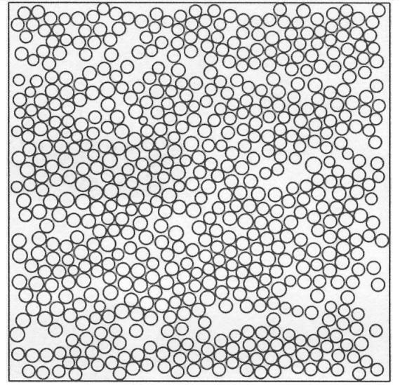
Figure 4: Mid-plane of shaft. Reprinted with permission from [26]. Copyright 2004, John Wiley and Sons.

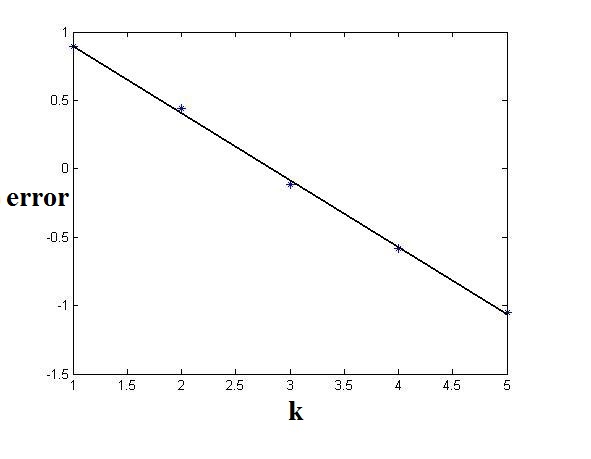
Figure 5: Decay of the error.

The simulations presented in [26] also numerically investigate the effect of the distance between the boundaries of $\omega$ and $\omega^{\ast}$. There it is found that the rate of convergence decreases as the distance is reduced and that the exponential convergence vanishes when $\omega$ and $\omega^{*}$ coincide.

$$\begin{array}[]{|l|l|l|l|l|l|}\hline\cr k&1&2&3&4&5\\ \hline\cr&$2.45\%$&$1.55\%$&$0.89\%$&$0.56\%$&$0.35\%$\\ \hline\cr\end{array}$$

Table 1. The error as function of the degree of harmonic polynomials charecterizing the boundary conditions $\varsigma_{\begin{subarray}{c}k\\ \end{subarray}}$.

So far we addressed only the case that the right hand side $f=0$ in the equation (1.1). The general case $f\neq 0$ can be easily reduced to the case $f=0.$ To this end we introduce the local particular solution of the differential equation (1.1) on each $\omega_{i}^{\ast}$ subject to a constant Neumann boundary condition over $\partial\omega_{i}^{*}$ determined according to the consistency condition. This is inexpensive to implement because the stiffness matrix has already been constructed together with its LU decomposition. We denote the local particular solution by $u_{\omega_{\scriptscriptstyle{i}}}$. Then the local approximation over $\omega_{i}$ used in the GFEM belongs to the hyperplane $\hat{\Psi}_{i}\oplus u_{\omega_{\scriptscriptstyle{i}}}$. Here the finite dimensional subspace $\hat{\Psi}_{i}$ is given by the optimal local bases constructed for the $A-$harmonic problem. As before this construction delivers a nearly exponential rate of convergence.

5 Homogenization of the $n$-width and exponential decay of approximation error in the pre-asymptotic regime

We identify the homogenization limit of the $n$-width and the corresponding optimal basis functions. These ideas are used to provide examples of exponential convergence of the approximation error when the characteristic length scale describing a heterogeneous medium is sufficiently small. In what follows we work in the general context and homogenization is described by $H$-convergence [17] or $G$-convergence [23]. We consider a sequence of coefficient matrices $A^{\epsilon}(x)$ in $\mathfrak{C}$ indexed by $\epsilon$, with $\epsilon=1/\ell$ for $\ell=1,2,\ldots$. Since we consider symmetric coefficient matrices the notions of $G$ convergence and $H$ convergence coincide and the class of coefficients $\mathfrak{C}$ is compact with respect to $H$-convergence see [17], [23]. In what follows we assume that the sequence $A^{\epsilon}$ $H$-converges to a homogenized coefficient matrix $A^{0}$ in $\mathfrak{C}$ and we write $A^{\epsilon}\overset{H}{\rightarrow}A^{0}$.

We describe the $n$-widths associated with the sequence $A^{\epsilon}$ and the $H$-limit $A^{0}$. For each $A^{\epsilon}$ we introduce the Hilbert space $\mathcal{H}_{\epsilon}$ defined to be all elements in $H_{A^{\epsilon}}(\omega^{*})/\mathbb{R}$ equipped with the energy inner product

$$(u,v)_{\mathcal{H}_{\epsilon}}=\int_{\omega^{*}}A^{\epsilon}\nabla u\cdot\nabla v\,dx$$ (5.1)

and norm $\|v\|_{\mathcal{H}_{\epsilon}}^{2}=(v,v)_{\mathcal{H}_{\epsilon}}$. The Hilbert space associated with $A^{0}$ is denoted by $\mathcal{H}_{0}$ and is defined to be all elements in $H_{A^{0}}(\omega^{*})/\mathbb{R}$ equipped with the energy inner product

$$(u,v)_{\mathcal{H}_{0}}=\int_{\omega^{*}}A^{0}\nabla u\cdot\nabla v\,dx$$ (5.2)

and norm $\|v\|_{\mathcal{H}_{0}}^{2}=(v,v)_{\mathcal{H}_{0}}$.

For each $A^{\epsilon}$ we introduce the restriction operator $P_{\epsilon}:\mathcal{H}_{\epsilon}\rightarrow H_{A^{\epsilon}}(\omega)/\mathbb{R}$ such that $P_{\epsilon}(u)(x)=u(x)$ for all $x\in\omega$ and $u\in\mathcal{H}_{\epsilon}$. As mentioned in the previous section the operator $P_{\epsilon}$ associated with $A^{\epsilon}$ is compact. For future reference the energy bilinear form defined on $H_{A^{\epsilon}}(\omega)/\mathbb{R}$ is given by

$$(u,v)_{\mathcal{E}_{\epsilon}(\omega)}=\int_{\omega}A^{\epsilon}\nabla u\cdot\nabla v\,dx$$ (5.3)

and we set $\|u\|_{\mathcal{E}_{\epsilon}(\omega)}^{2}=(u,u)_{\mathcal{E}_{\epsilon}(\omega)}$. Similarly, for the $H$-limit $A^{0}$ we introduce the compact operator given by the restriction $P_{0}:\mathcal{H}_{0}\rightarrow H_{A^{0}}(\omega)/\mathbb{R}$ such that $P_{0}(u)(x)=u(x)$ for all $x\in\omega$ and $u\in\mathcal{H}_{0}$. The energy bilinear form defined on $H_{A^{0}}(\omega)$ is given by

$$(u,v)_{\mathcal{E}_{0}(\omega)}=\int_{\omega}A^{0}\nabla u\cdot\nabla v\,dx$$ (5.4)

and we set $\|u\|_{\mathcal{E}_{0}(\omega)}^{2}=(u,u)_{\mathcal{E}_{0}(\omega)}$.

The $n$ width associated with the coefficients $A^{\epsilon}$ is given by

$$d_{n}^{\epsilon}(\omega,\omega^{*})=\inf_{S(n)\subset H_{A^{\epsilon}}(\omega)/\mathbb{R}}\sup_{u\in\mathcal{H}_{\epsilon}}\inf_{\chi\in S(n)}\frac{\|P_{\epsilon}u-\chi\|_{\mathcal{E_{\epsilon}}(\omega)}}{\|u\|_{\mathcal{H}_{\epsilon}}}.$$ (5.5)

The optimal local approximation space $\Psi^{\epsilon}_{n}(\omega)$ associated with $A^{\epsilon}$ is described in terms of the eigenfunctions associated with the following spectral problem. We introduce the adjoint operator $P_{\epsilon}^{*}:H_{A^{\epsilon}}(\omega)/\mathbb{R}\rightarrow\mathcal{H}_{\epsilon}$ and the operator $P_{\epsilon}^{*}P_{\epsilon}$ is a self adjoint non-negative compact map taking $\mathcal{H}_{\epsilon}$ into itself. The eigenfunctions and eigenvalues are denoted by $\{\varphi^{\epsilon}_{i}\}_{i=1}^{\infty}$ and $\{\lambda^{\epsilon}_{i}\}_{i=1}^{\infty}$ and satisfy the problem

$$(P_{\epsilon}^{*}P_{\epsilon}\varphi_{i}^{\epsilon},\delta)_{\scriptscriptstyle{\mathcal{H}_{\epsilon}}} = \lambda^{\epsilon}_{i}(\varphi_{i}^{\epsilon},\delta)_{\mathcal{H}_{\epsilon}}\hbox{, $\forall\delta\in\mathcal{H}_{\epsilon}$}.$$ (5.6)

The non-zero eigenvalues of $P_{\epsilon}^{*}P_{\epsilon}$ are listed according to decreasing order of magnitude

$$\lambda_{1}^{\epsilon}\geq\lambda_{2}^{\epsilon}\geq\ldots>0.$$ (5.7)

The optimal approximation space is given by $\Psi^{\epsilon}_{n}(\omega)=span\{\psi^{\epsilon}_{1},\ldots,\psi^{\epsilon}_{n}\}$, where $\psi^{\epsilon}_{i}=P_{\epsilon}\varphi^{\epsilon}_{i}$ and $d_{n}^{\epsilon}(\omega,\omega^{*})=\sqrt{\lambda_{n+1}^{\epsilon}}$. The $n$ width associated with the coefficient $A^{0}$ is given by

$$d_{n}^{0}(\omega,\omega^{*})=\inf_{S(n)\subset H_{A^{0}}(\omega)}\sup_{u\in\mathcal{H}_{0}}\inf_{\chi\in S(n)}\frac{\|P_{0}u-\chi\|_{\mathcal{E}_{0}(\omega)}}{\|u\|_{\mathcal{H}_{0}}}.$$ (5.8)

The optimal local approximation space $\Psi^{0}_{n}(\omega)$ associated with $A^{0}$ is described in terms of the eigenfunctions associated with the following spectral problem. We introduce the adjoint operator $P_{0}^{*}:H_{A^{\epsilon}}(\omega)/\mathbb{R}\rightarrow\mathcal{H}_{0}$ and the operator $P_{0}^{*}P_{0}$ is a self adjoint non-negative compact map taking $\mathcal{H}_{0}$ into itself. The eigenfunctions and eigenvalues are denoted by $\{\varphi^{0}_{i}\}_{i=1}^{\infty}$ and $\{\lambda^{0}_{i}\}_{i=1}^{\infty}$ and satisfy the problem

$$(P_{0}^{*}P_{0}\varphi^{0}_{i},\delta)_{\scriptscriptstyle{\mathcal{H}_{0}}} = \lambda^{0}_{i}(\varphi_{i}^{0},\delta)_{\mathcal{H}_{0}}\hbox{, $\forall\delta\in\mathcal{H}_{0}$}.$$ (5.9)

The non-zero eigenvalues of $P_{0}^{*}P_{0}$ are listed according to decreasing order of magnitude

$$\lambda_{1}^{0}\geq\lambda_{2}^{0}\geq\ldots>0.$$ (5.10)

The optimal approximation space is given by $\Psi^{0}_{n}(\omega)=span\{\psi^{0}_{1},\ldots,\psi^{0}_{n}\}$, where $\psi^{0}_{i}=P_{0}\varphi^{0}_{i}$ and $d_{n}^{0}(\omega,\omega^{*})=\sqrt{\lambda_{n+1}^{0}}$. The homogenization limit of $n$-widths and optimal approximations is given by the following theorem.

Theorem 5.1.

Suppose that the coefficient matrices $A^{\epsilon}(x)$ in $\mathfrak{C}$ $H$-converge to $A^{0}(x)$ in $\mathfrak{C}$ as $\epsilon\rightarrow 0$. Then there exists a subsequence of coefficients $A^{\epsilon}\overset{H}{\rightarrow}A^{0}$ such that

$$\lambda_{i}^{\epsilon}\rightarrow\lambda_{i}^{0} \varphi_{i}^{\epsilon}\rightharpoonup\varphi_{i}^{0},\hbox{ weakly in $H^{1}(\omega^{*})$, for $i=1,2\ldots$}$$ and (5.11)

Hence

$$\lim_{\epsilon\rightarrow 0}d_{n}^{\epsilon}(\omega,\omega^{*})=d_{n}^{0}(\omega,\omega^{*})$$ (5.12)

and each function in the optimal basis for $A^{\epsilon}$ given by $\Psi^{\epsilon}_{n}(\omega)=span\{\psi^{\epsilon}_{1},\ldots,\psi^{\epsilon}_{n}\}$ converges weakly in $H^{1}(\omega)$ to the corresponding function in the optimal basis for $A^{0}$ given by $\Psi^{0}_{n}(\omega)=span\{\psi^{0}_{1},\ldots,\psi^{0}_{n}\}$.

Proof. The proof proceeds in three steps.

Step 1. We start by fixing the index $i$ and state the following Lemma.

Lemma 5.1.

Suppose $A^{\epsilon}\overset{H}{\rightarrow}A^{0}$. For $i$ fixed, consider the associated eigenfunction and eigenvalue $(\varphi^{\epsilon}_{i},\lambda_{i}^{\epsilon})$ of $P_{\epsilon}^{*}P_{\epsilon}$. Sending $\epsilon\rightarrow 0$ and passing to subsequences as necessary there exists a positive number $\overline{\lambda}_{i}$ and function $\overline{\varphi}_{i}\in\mathcal{H}_{0}$ for which

$$\lambda_{i}^{\epsilon}\rightarrow\overline{\lambda}_{i} \varphi_{i}^{\epsilon}\rightharpoonup\overline{\varphi}_{i},\hbox{weakly in $H^{1}(\omega^{*})$},$$ and (5.13)

and

$$(P_{0}^{*}P_{0}\overline{\varphi}_{i},\delta)_{\scriptscriptstyle{\mathcal{H}_{0}}} = \overline{\lambda}_{i}(\overline{\varphi}_{i},\delta)_{\mathcal{H}_{0}}\hbox{, $\forall\delta\in\mathcal{H}_{0}$}.$$ (5.14)

Before proceeding with the proof of Lemma 5.1 we state the following two compensated compactness results presented in the work of Murat and Tartar [17] for later reference.

Lemma 5.2.

Let $\epsilon\rightarrow 0$, $D$ be any open subset of $\mathbb{R}^{d}$, and $\xi^{\epsilon}$, $v^{\epsilon}$, be sequences such that

$$\xi^{\epsilon}\in L^{2}(D)^{d},$$

$$\xi^{\epsilon}\rightharpoonup\xi^{0}\hbox{ weakly in $L^{2}(D)^{d}$},$$

$$div\xi^{\epsilon}\rightarrow div\xi^{0}\hbox{ strongly in $H^{-1}(D)$},$$ (5.15)

and

$$v^{\epsilon}\in H^{1}(D),$$

$$v^{\epsilon}\rightharpoonup v^{0}\hbox{ weakly in $H^{1}(D)$}.$$ (5.16)

Then

$$\int_{D}\xi^{\epsilon}\cdot\nabla v^{\epsilon}\eta\,dx\rightarrow\int_{D}\xi^{0}\cdot\nabla v^{0}\eta\,dx,\hbox{ $\forall\eta\in C_{0}^{\infty}(D)$}.$$ (5.17)

Lemma 5.3.

Suppose that $A^{\epsilon}(x)$ in $\mathfrak{C}$ $H$-converges to $A^{0}(x)$ in $\mathfrak{C}$ as $\epsilon\rightarrow 0$. Assume that $u^{\epsilon}\in H^{1}(D)$, $f^{\epsilon}\in H^{-1}(D)$ and

$$-div(A^{\epsilon}\nabla u^{\epsilon}) = f^{\epsilon},\hbox{ in $D$,}$$

$$u^{\epsilon} \rightharpoonup u^{0}\hbox{ weakly in $H^{1}(D)$},$$

$$f^{\epsilon} \rightarrow f^{0}\hbox{ strongly in $H^{-1}(D)$},$$ (5.18)

for $\epsilon\rightarrow 0$. Then

$$A^{\epsilon}\nabla u^{\epsilon} \rightharpoonup A^{0}\nabla u^{0}\hbox{ weakly in $L^{2}(D)^{d}$,}$$

$$\int_{D}(A^{\epsilon}\nabla u^{\epsilon}\cdot\nabla u^{\epsilon})\eta\,dx \rightarrow \int_{D}(A^{0}\nabla u^{0}\cdot\nabla u^{0})\eta\,dx,\hbox{ $\forall\eta\in C_{0}^{\infty}(D)$ and}$$

$$A^{\epsilon}\nabla u^{\epsilon}\cdot\nabla u^{\epsilon} \rightharpoonup A^{0}\nabla u^{0}\cdot\nabla u^{0}\hbox{ weakly in $L^{1}_{loc}(D)$}.$$ (5.19)

Proof of Lemma 5.1. Following section 3 the we write (5.6) as

$$\int_{\omega}A^{\epsilon}\nabla\varphi^{\epsilon}_{i}\cdot\nabla\delta\,dx=\lambda^{\epsilon}_{i}\int_{\omega^{*}}A^{\epsilon}\nabla\varphi^{\epsilon}_{i}\cdot\nabla\delta\,dx,\,\,\hbox{$\forall\delta\in\mathcal{H}_{\epsilon}$}.$$ (5.20)

Now consider the sequence of eigenfunctions $\{\varphi^{\epsilon}_{i}\}_{\epsilon>0}$ for (5.20) and with out loss of generality we normalize $\varphi_{i}^{\epsilon}$ so that

$$\int_{\omega^{*}}A^{\epsilon}\nabla\varphi_{i}^{\epsilon}\cdot\nabla\varphi_{i}^{\epsilon}\,dx=1 \lambda_{i}^{\epsilon}=\int_{\omega}A^{\epsilon}\nabla\varphi_{i}^{\epsilon}\cdot\nabla\varphi_{i}^{\epsilon}\,dx.$$ and (5.21)

From (5.21) we can extract a subsequence $\{\varphi_{i}^{\epsilon}\}_{\epsilon>0}$ and $\overline{\varphi}_{i}\in H^{1}(\omega^{*})$ such that $\varphi_{i}^{\epsilon}\rightharpoonup\overline{\varphi}_{i}$ weakly in $H^{1}(\omega^{*})$. Since $\varphi_{i}^{\epsilon}\in\mathcal{H}_{\epsilon}\subset H^{1}(\omega^{*})$ we apply Lemma 5.3 to deduce that for $\epsilon\rightarrow 0$,

$$A^{\epsilon}\nabla\varphi_{i}^{\epsilon} \rightharpoonup A^{0}\nabla\overline{\varphi}_{i}^{,}\hbox{ weakly in $L^{2}(\omega^{*})^{d},$}$$

$$\int_{\omega^{*}}(A^{\epsilon}\nabla\varphi_{i}^{\epsilon}\cdot\nabla\varphi_{i}^{\epsilon})\delta\,dx \rightharpoonup \int_{\omega^{*}}(A^{0}\nabla\overline{\varphi}_{i}\cdot\nabla\overline{\varphi}_{i})\delta\,dx,\hbox{$\forall\delta\in C_{0}^{\infty}(\omega^{*})$ and}$$

$$A^{\epsilon}\nabla\varphi_{i}^{\epsilon}\cdot\nabla\varphi_{i}^{\epsilon} \rightharpoonup A^{0}\nabla\overline{\varphi}_{i}\cdot\nabla\overline{\varphi}_{i},\hbox{ weakly in $L^{1}(\omega)$,}$$ (5.22)

and $\overline{\varphi}_{i}\in\mathcal{H}_{0}$, hence

$$\lambda_{i}^{\epsilon}\rightarrow\int_{\omega}A^{0}\nabla\overline{\varphi}_{i}\cdot\nabla\overline{\varphi}_{i}\,dx=\overline{\lambda}_{i}.$$ (5.23)

To finish the proof we show that $\overline{\varphi}_{i}$ and $\overline{\lambda}_{i}$ are solutions of (5.14). Consider any $g\in H^{1/2}(\partial\omega^{*})$ and $\delta^{\epsilon}\in\mathcal{H}_{\epsilon}$ such that $\delta^{\epsilon}=g$ on $\partial\omega^{*}$. We write $\delta^{\epsilon}=w^{\epsilon}+v$ where

$$v=g\hbox{ on }\partial\omega^{*} \Delta v=0\hbox{ in }\omega^{*},$$ and (5.24)

and $w^{\epsilon}\in H_{0}^{1}(\omega^{*})$, where

$$-\mathrm{div}(A^{\epsilon}\nabla w^{\epsilon})=\mathrm{div}(A^{\epsilon}\nabla v),$$ (5.25)

in $\omega^{*}$.

For any sequence of coefficients $A^{\epsilon}\in\mathfrak{C}$ Theorem 1 of [16] shows that the sequence $\nabla w^{\epsilon}$ enjoys the higher integrability given by the following Lemma.

Lemma 5.4.

There is an interval $Q>p>2$ such that for $v\in W^{1,p}(\omega^{*})$ then

$$\sup_{\varepsilon>0}\{\|\nabla w^{\epsilon}\|_{L^{p}(\omega^{*})}\}<\infty.$$ (5.26)

Here the interval is independent of $\epsilon$ and depends only on $\omega^{*}$, $\alpha$ and $\beta$.

Now consider a dense subset $S$ of $H^{1/2}(\partial\omega^{*})$ such that $g\in S$ implies that the solution $v$ of (5.24) belongs to $W^{1,p}(\omega^{*})$. Then $\|\nabla\delta^{\epsilon}\|_{L^{p}(\omega^{*})}\leq\|\nabla w^{\epsilon}\|_{L^{p}(\omega^{*})}+\|\nabla v\|_{L^{p}(\omega^{*})}$ and Lemma 5.4 implies that the associated sequence $\{\delta^{\epsilon}\}_{\epsilon>0}$ satisfies

$$\sup_{\varepsilon>0}\{\|\nabla\delta^{\epsilon}\|_{L^{p}(\omega^{*})}\}<\infty.$$ (5.27)

Additionally passing to a subsequence if necessary we see that there is an element $\delta\in H^{1}(\omega^{*})$ for which $\delta^{\epsilon}\rightharpoonup\delta$ weakly in $H^{1}(\omega^{*})$. Next an application of Lemma 5.3 shows that $\delta\in\mathcal{H}_{0}$ and an application of 5.2 to the sequences $\{A^{\epsilon}\nabla\varphi^{\epsilon}_{i}\}_{\epsilon>0}$ and $\{\delta^{\epsilon}\}_{\epsilon>0}$ gives

$$\int_{\omega^{*}}(A^{\epsilon}\nabla\varphi_{i}^{\epsilon}\cdot\nabla\delta^{\epsilon})\eta\,dx \rightarrow \int_{\omega^{*}}(A^{0}\nabla\overline{\varphi}_{i}\cdot\nabla\delta)\eta\,dx\hbox{ $\forall\eta\in C_{0}^{\infty}(\omega^{*})$}.$$ (5.28)

From (5.27) we deduce that $\{A^{\epsilon}\nabla\varphi_{i}^{\epsilon}\cdot\nabla\delta^{\epsilon}\}_{\epsilon>0}$ is equiintegrable on $\omega^{*}$ and it follows that

$$\int_{\omega}A^{\epsilon}\nabla\varphi_{i}^{\epsilon}\cdot\nabla\delta^{\epsilon} \rightarrow \int_{\omega}A^{0}\nabla\overline{\varphi}_{i}\cdot\nabla\delta\,dx,$$ (5.29)

$$\int_{\omega^{*}}A^{\epsilon}\nabla\varphi_{i}^{\epsilon}\cdot\nabla\delta^{\epsilon} \rightarrow \int_{\omega^{*}}A^{0}\nabla\overline{\varphi}_{i}\cdot\nabla\delta\,dx.$$ (5.30)

From (5.23), (5.29), (5.30), we deduce that

$$\int_{\omega}A^{0}\nabla\overline{\varphi}_{i}\cdot\nabla\delta\,dx=\overline{\lambda}_{i}\int_{\omega^{*}}A^{0}\nabla\overline{\varphi}_{i}\cdot\nabla\delta\,dx,$$ (5.31)

or equivalently

$$(P_{0}^{*}P_{0}\overline{\varphi}_{i},\delta)_{\scriptscriptstyle{\mathcal{H}_{0}}} = \overline{\lambda}_{i}(\overline{\varphi}_{i},\delta)_{\mathcal{H}_{0}}$$ (5.32)

for all test functions $\delta$ belonging to $\mathcal{H}_{0}$ with traces in $S$, i.e., $\delta=g$ on $\partial\omega^{*}$, for $g\in S$. Lemma 5.1 now follows from the density of $S$ in $H^{1/2}(\partial\omega^{*})$.

Step 2. We apply Lemma 5.1 together with a diagonalization argument to extract a subsequence still denoted by $(\lambda^{\epsilon}_{i},\varphi^{\epsilon}_{i})$, such that for every $i=1,2\ldots$

$$\lambda^{\epsilon}_{i}\rightarrow\overline{\lambda}_{i}\hbox{ and }\varphi^{\epsilon}_{i}\rightharpoonup\overline{\varphi}_{i}\hbox{ weakly in $H^{1}(\omega^{*})$}$$ (5.33)

where $(\overline{\lambda}_{i},\overline{\varphi}_{i})$ are solutions of (5.14) and

$$\overline{\lambda}_{1}\geq\overline{\lambda}_{2}\geq\ldots>0.$$ (5.34)

Step 3. The final step is to show that all the eigenfunctions and eigenvalues of the operator $P_{0}^{*}P_{0}$ are given by $(\overline{\lambda}_{i},\overline{\varphi}_{i})$ obtained in step 2. We argue by contradiction and assume that there is an eigenvalue $\lambda$ of $P_{0}^{*}P_{0}$ for which $\lambda\not=\overline{\lambda}_{i}$ for every $i=1,2,\ldots$. Let $\varphi$ be a corresponding normalized eigenvector i.e., $(P_{0}^{*}P_{0}\varphi,\delta)_{\mathcal{H}_{0}}=\lambda(\varphi,\delta)_{\mathcal{H}_{0}}$, for every $\delta\in\mathcal{H}_{0}$ and $\|\varphi\|_{\mathcal{H}_{0}}=1$. Then there is an integer $m$ such that

$$\lambda>\overline{\lambda}_{m+1}.$$ (5.35)

To proceed we introduce the Rayleigh quotient for $v\in\mathcal{H}_{\epsilon}$ given by

$$R_{\epsilon}(v)=\frac{(P_{\epsilon}^{*}P_{\epsilon}v,v)_{\mathcal{H}_{\epsilon}}}{\|v\|^{2}_{\mathcal{H}_{\epsilon}}}$$ (5.36)

and the eigenvalues of $P_{\epsilon}^{*}P_{\epsilon}$ listed in decreasing order are given by

$$\lambda^{\epsilon}_{i}=\max_{v\in\mathcal{H}_{\epsilon}\perp\varphi_{1}^{\epsilon},\ldots\varphi_{i-1}^{\epsilon}}R_{\epsilon}(v).$$ (5.37)

We establish the contradiction first under the extra assumption that the gradient of $\varphi\in\mathcal{H}_{0}$ enjoys higher integrability and belongs to $W^{1,p}(\omega^{*})$ for $p>2$. We then indicate how to proceed without this assumption.

Introduce $u^{\epsilon}\in\mathcal{H}_{\epsilon}$ such that $u^{\epsilon}=\varphi$ on $\partial\omega^{*}$. On passing to a further subsequence if needed we apply Theorem 5.3 to see that

$$u^{\epsilon}\rightharpoonup\varphi\hbox{ weakly in $H^{1}(\omega^{*})$ and}$$

$$(P_{\epsilon}^{*}P_{\epsilon}u^{\epsilon},u^{\epsilon})_{\mathcal{H}_{\epsilon}}=\int_{\omega}A^{\epsilon}\nabla u^{\epsilon}\cdot\nabla u^{\epsilon}\,dx\rightarrow\int_{\omega}A^{0}\nabla\varphi\cdot\nabla\varphi\,dx=\lambda.$$ (5.38)

Noting from that $\varphi\in W^{1,p}(\omega^{*})$ we observe from the arguments preceding (5.27) that

$$\sup_{\varepsilon>0}\{\|\nabla u^{\epsilon}\|_{L^{p}(\omega^{*})}\}<\infty.$$ (5.39)

Thus the sequence $\{A^{\epsilon}\nabla u^{\epsilon}\cdot\nabla u^{\epsilon}\}_{\epsilon>0}$ is equiintegrable on $\omega^{*}$ and we conclude that

$$(u^{\epsilon},u^{\epsilon})_{\mathcal{H}_{\epsilon}}=\int_{\omega^{*}}A^{\epsilon}\nabla u^{\epsilon}\cdot\nabla u^{\epsilon}\,dx\rightarrow\int_{\omega^{*}}A^{0}\nabla\varphi\cdot\nabla\varphi\,dx=1$$ (5.40)

so

$$\lim_{\epsilon\rightarrow 0}R_{\epsilon}(u^{\epsilon})=\lambda.$$ (5.41)

Now introduce $v^{\epsilon}\in\mathcal{H}_{\epsilon}$ given by

$$v^{\epsilon}=u^{\epsilon}-\sum_{i=1}^{m}(u^{\epsilon},\varphi^{\epsilon}_{i})_{\scriptscriptstyle{\mathcal{H}_{\epsilon}}}\varphi^{\epsilon}_{i}$$ (5.42)

As before we make use of the equiintegrability of $\{A^{\epsilon}\nabla u^{\epsilon}\cdot\nabla\varphi_{i}^{\epsilon}\}_{\epsilon>0}$ on $\omega^{*}$ together with Lemma 5.3 to find that

$$(u^{\epsilon},\varphi^{\epsilon}_{i})_{\mathcal{H}_{\epsilon}}=\int_{\omega^{*}}A^{\epsilon}\nabla u^{\epsilon}\cdot\nabla\varphi_{i}^{\epsilon}\,dx\rightarrow\int_{\omega^{*}}A^{0}\nabla\varphi\cdot\nabla\overline{\varphi}_{i}\,dx=(\varphi,\overline{\varphi}_{i})_{\mathcal{H}_{0}}.$$ (5.43)

Since $\lambda\not=\overline{\lambda}_{i}$ for all $i$, it follows from the orthogonality of eigenvectors of $P_{0}^{*}P_{0}$ that $(\varphi,\overline{\varphi}_{i})_{\mathcal{H}_{0}}=0$ for $i=1,2,\ldots,m$ and we deduce that

$$(u^{\epsilon},\varphi^{\epsilon}_{i})_{\mathcal{H}_{\epsilon}}\rightarrow 0.$$ (5.44)

Writing

$$\|v^{\epsilon}\|_{\mathcal{H}_{\epsilon}}^{2}=\|u^{\epsilon}\|_{\mathcal{H}_{\epsilon}}-\sum_{i=1}^{m}(u^{\epsilon},\varphi^{\epsilon}_{i})_{\scriptscriptstyle{\mathcal{H}_{\epsilon}}}^{2},$$

$$(P_{\epsilon}^{*}P_{\epsilon}v^{\epsilon},v^{\epsilon})_{\mathcal{H}_{\epsilon}}=(P_{\epsilon}^{*}P_{\epsilon}u^{\epsilon},u^{\epsilon})_{\mathcal{H}_{\epsilon}}-\sum_{i=1}^{m}\lambda_{i}^{\epsilon}(u^{\epsilon},\varphi^{\epsilon}_{i})_{\scriptscriptstyle{\mathcal{H}_{\epsilon}}}^{2}$$ (5.45)

and sending $\epsilon$ to zero using (5.38), (5.40), and (5.44) we conclude that

$$\lim_{\epsilon\rightarrow 0}R_{\epsilon}(v^{\epsilon})=\lambda.$$ (5.46)

On the other hand

$$(v^{\epsilon},\varphi^{\epsilon}_{i})_{\mathcal{H}_{\epsilon}}=0,\hbox{ for $i=1,2,\ldots,m$}$$ (5.47)

so from (5.37) we get $\lambda^{\epsilon}_{m+1}\geq\lambda$ and taking limits gives $\overline{\lambda}_{m+1}\geq\lambda$ which is a contradiction to the original assumption $\lambda>\overline{\lambda}_{m+1}$.

We now remove the higher integrability assumption on the gradient of $\varphi\in\mathcal{H}_{0}$. For this case consider a sequence $s=1/\ell,\ell=1,2,\ldots$ and functions $\delta_{s}\in W^{1,p}(\omega^{*})$ that converge to $\varphi$ in $W^{1,2}(\omega^{*})$ as $s$ goes to zero. Choose $u_{s}^{\epsilon}\in\mathcal{H}_{\epsilon}$ such that $u^{\epsilon}_{s}=\delta_{s}$ on $\partial\omega^{*}$. Then construct $v_{s}^{\epsilon}$ according to

$$v_{s}^{\epsilon}=u_{s}^{\epsilon}-\sum_{i=1}^{m}(u_{s}^{\epsilon},\varphi_{i}^{\epsilon})_{\mathcal{H}_{\epsilon}}\varphi^{\epsilon}_{i}.$$ (5.48)

As before $(v_{s}^{\epsilon},\varphi_{i}^{\epsilon})_{\mathcal{H}_{\epsilon}}=0$, for $i=1,\ldots,m$ and $\lambda_{m+1}^{\epsilon}\geq R_{\epsilon}(v_{s}^{\epsilon})$. Following previous arguments one deduces that the sequence $u_{s}^{\epsilon}$ is bounded in $W^{1,p}(\omega^{*})$ and on passing to subsequences as necessary

$$u_{s}^{\epsilon}\rightharpoonup u_{s}\hbox{ weakly in $H^{1}(\omega^{*})$ where $u_{s}\in\mathcal{H}_{0}$},$$

$$(P_{\epsilon}^{*}P_{\epsilon}u_{s}^{\epsilon},u_{s}^{\epsilon})_{\mathcal{H}_{\epsilon}}\rightarrow\int_{\omega}A^{0}\nabla u_{s}\cdot\nabla u_{s}\,dx,$$

$$(u_{s}^{\epsilon},u_{s}^{\epsilon})_{\mathcal{H}_{\epsilon}}\rightarrow(u_{s},u_{s})_{\mathcal{H}_{0}},\hbox{ and}$$

$$(u_{s}^{\epsilon},\varphi_{i}^{\epsilon})_{\mathcal{H}_{\epsilon}}\rightarrow(u_{s},\overline{\varphi}_{i})_{\mathcal{H}_{0}},\hbox{ for $i=1,\ldots,m$}$$ (5.49)

and

$$\lim_{\varepsilon\rightarrow 0}R_{\epsilon}(v_{s}^{\epsilon})=\frac{\int_{\omega}\,A^{0}\nabla u_{s}\cdot\nabla u_{s}dx-\sum_{i=1}^{m}\overline{\lambda}_{i}(u_{s},\overline{\varphi}_{i})_{\mathcal{H}_{0}}^{2}}{(u_{s},u_{s})_{\mathcal{H}_{0}}^{2}-\sum_{i=1}^{m}(u_{s},\overline{\varphi}_{i})_{\mathcal{H}_{0}}^{2}}.$$ (5.50)

Since $\delta_{s}$ converges strongly in $H^{1}(\omega^{*})$ to $\varphi$ it follows from the uniqueness of solution of the Dirichlet boundary value problem for $A^{0}$ harmonic functions that $u_{s}$ converges strongly to $\varphi$ in $\mathcal{H}_{0}$ thus

$$\overline{\lambda}_{m+1}\geq\lim_{s\rightarrow 0}\lim_{\varepsilon\rightarrow 0}R_{\epsilon}(v_{s}^{\epsilon})=\lambda$$ (5.51)

and we arrive at a contradiction and Theorem 5.1 is proved.

We conclude by applying the homogenization of $n$-width theorem to construct an example that shows exponential decay of the approximation error in the pre-asymptotic regime. We consider a heterogeneous medium with characteristic length scale $\epsilon>0$. To fix ideas we work in two dimensions and suppose that the associated sequence of coefficients $A^{\epsilon}$ is such that it $H$-converges to a constant effective conductivity $A^{0}$ matrix as $\epsilon\rightarrow 0$. In the coordinate system corresponding to the eigenvectors $e^{1}$, $e^{2}$ of $A^{0}$ we have $A^{0}=a_{1}e^{1}\otimes e^{1}+a_{2}e^{2}\otimes e^{2}$ and we set $b=a_{2}/a_{1}$. To fix ideas we suppose that $\omega^{*}$ is the ellipsoid $E_{r^{*}}=\{(x_{1},x_{2});x_{1}^{2}+x_{2}^{2}/b=r^{*}\}$ and $\omega\subset\omega^{*}$ is the concentric ellipsoid $E_{r}=\{(x_{1},x_{2});x_{1}^{2}+x_{2}^{2}/b=r\}$ with $r<r^{*}$. For $z=x+iy$ recall the harmonic polynomials $w_{j}(x_{1},x_{2})=\Re{z^{j}}=r^{j}\cos{(j\theta)}$, $\hat{w}_{j}(x_{1},x_{2})=\Im{z^{j}}=r^{j}\sin{(j\theta)}$, for $j=1,\ldots,n$. Calculation shows that the optimal basis associated with the $n$ width for $A^{0}$ is given by the $A^{0}$ harmonic polynomials $v_{j}=w_{j}(x_{1},x_{2}/\sqrt{b})$, $\hat{v}_{j}=\hat{w}_{j}(x_{1},x_{2}/\sqrt{b})$ and eigenvalues $\lambda_{j}=e^{-2|\ln{\frac{r}{r^{*}}}|j}$, $j=1,\ldots,n$ of

$$\int_{E_{r}}A^{0}\nabla\varphi_{j}\cdot\nabla\delta\,dx=\lambda_{j}\int_{E_{r^{*}}}A^{0}\nabla\varphi_{j}\cdot\nabla\delta\,dx,$$ (5.52)

for all $\delta\in H_{A^{0}}(\omega^{*})$. It follows from Theorem 3.1 that the decay of approximation error for the optimal basis associated with the homogenized coefficient $A^{0}$ is

$$e^{-|\ln{\frac{r}{r^{*}}}|(n+1)}.$$ (5.53)

Now we denote the $n$ width associated with the optimal basis for $A^{\epsilon}$ by $d_{n}^{\epsilon}(E_{r},E_{r^{*}})$. Direct application of Theorem 5.1 together with (5.53) gives the the following bound on the pre-asymptotic rate of approximation error.

Theorem 5.2.

Given $N>0$ and tolerance $\tau>0$ there exist an $\epsilon>0$ such that for $1\leq n\leq N$, that

$$e^{-|\ln{\frac{r}{r^{*}}}|(n+1)}-\tau\leq d_{n}^{\epsilon}(E_{r},E_{r^{*}})\leq e^{-|\ln{\frac{r}{r^{*}}}|(n+1)}+\tau.$$ (5.54)

6 Implementation in the pre-asymptotic regime and more examples of exponential convergence

In this section we discuss a method for computational approximation that employs the optimal basis for the homogenized problem to construct approximation spaces for composites with heterogeneities on the length scale $\epsilon>0$ relative to the size of $\omega^{*}$. We work in the general context and consider a sequence of coefficient matrices $\{A^{\epsilon}\}_{\epsilon>0}\in\mathfrak{C}$ that $H$-converge to a homogenized coefficient matrix $A^{0}\in\mathfrak{C}$. For this case we recall the eigenfunctions $\varphi^{\epsilon}_{i}$ of (5.6) and $\varphi^{0}_{i}$ of (5.9) associated with $A^{\epsilon}$ and $A^{0}$ respectively. For $\epsilon>0$ fixed the optimal approximation space is given by the span of the restriction of the functions $\varphi^{\epsilon}_{i}$, $i=1,\ldots,n$ to $\omega$. However in general it is known that the direct numerical computation of eigenfunctions is computationally expensive. Instead we introduce the functions $\phi_{i}^{\epsilon}\in H_{A^{\epsilon}}(\omega^{*})/\mathbf{R}$ such that $\phi_{i}^{\epsilon}=\varphi_{i}^{0}$ on $\partial\omega^{*}$, for $i=1,\ldots,n$. We then define the approximation space $V_{\epsilon}^{n}(\omega)$ by

$$V_{\epsilon}^{n}(\omega)=span\left\{u^{\epsilon}_{i}=P\phi_{i}^{\epsilon},\,\,\,i=1,\ldots,n\right\}$$ (6.1)

and state the following approximation theorem

Theorem 6.1.

Given a tolerance $\tau>0$ there exists an $\overline{\varepsilon}>0$ such that $\forall\epsilon<\overline{\epsilon}$

$$\|u_{i}^{\epsilon}-\varphi_{i}^{\epsilon}\|_{\mathcal{E}(\omega)}<\tau$$ (6.2)

We point out that this theorem remains the same if we choose $\phi_{i}^{\epsilon}\in H_{A^{\epsilon}}(\omega^{*})/\mathbb{R}$ such that $n\cdot A^{\varepsilon}\nabla\phi_{i}^{\epsilon}=n\cdot A^{0}\nabla\varphi_{i}^{0}$ on $\partial\omega^{*}$, for $i=1,\ldots,n$. When the homogenized coefficient $A^{0}$ is sufficiently simple e.g., $A^{0}$ is a constant, and $\omega$ and $\omega^{*}$ are concentric ellipsoids, the optimal approximation space for the homogenized problem is given by explicit transcendental functions. And it follows that the associated approximation space $V^{n}(\omega)$ is far less expensive to compute than the eigenvalue problem associated with the optimal approximation space. For these situations Theorem 6.1 shows that $V_{\epsilon}^{n}(\omega)$ can be used provided that $\epsilon$ is sufficiently small. We point out that the traces of the approximations $\phi_{i}^{\varepsilon}$ are indeed smooth on $\partial\omega^{*}$ noting that this is exactly the assumption made in section when considering the accuracy of the approximate local basis given in section 4. For fiber reinforced composite materials it is clear that the size of $\omega$ needs to be chosen sufficiently large so that the relative length scale of the fiber cross sections as characterized by $\varepsilon$ is sufficiently small.

We now give the proof of Theorem 6.1. Recall from Theorem 5.1 that $\varphi_{i}^{\epsilon}\rightharpoonup\varphi_{i}^{0}$ in $H^{1}(\omega^{*})$, hence $\varphi_{i}^{\epsilon}\rightarrow\varphi_{i}^{0}$ in $L^{2}(\omega^{*})$. On the other hand since $A^{\epsilon}$ $H$-converges to $A^{0}$ it follows from Theorem 5.3 that $\phi_{i}^{\epsilon}\rightharpoonup\varphi_{i}^{0}$ in $H^{1}(\omega^{*})$, hence $\phi_{i}^{\epsilon}\rightarrow\varphi_{i}^{0}$ in $L^{2}(\omega^{*})$. Application of the Caccioppoli inequality delivers

$$\|u_{i}^{\epsilon}-\varphi_{i}^{\epsilon}\|_{\mathcal{E}(\omega)}<(4(\beta)^{1/2}/\sigma\rho)\|\phi_{i}^{\epsilon}-\varphi_{i}^{\epsilon}\|_{L^{2}(\omega^{*})}$$

$$\leq(4(\beta)^{1/2}/\sigma\rho)\left(\|\phi_{i}^{\epsilon}-\varphi_{i}^{0}\|_{L^{2}(\omega^{*})}+\|\varphi_{i}^{\epsilon}-\varphi_{i}^{0}\|_{L^{2}(\omega^{*})}\right)$$ (6.3)

and Theorem 6.1 is proved.

In the numerical example presented at the end of section 4 we have assumed that the homogenized equation is given by the Laplace equation, i.e., $A^{0}=I$ and that the functions $\varphi_{i}^{0}=\varsigma_{i}$ are the traces of harmonic polynomials.

Consider a family of heterogeneous media with characteristic length scale $\epsilon>0$. We suppose as before $A^{\epsilon}$ is $H$-convergent and converges to a constant effective conductivity $A^{0}$ matrix as $\epsilon\rightarrow 0$. We take $\omega^{*}$ to be the unit square and $\omega$ to be a concentric square of side length $\sigma<1$ contained inside $\omega^{*}$. We suppose that $\sigma$ is such that we can fit concentric ellipsoids $E_{r}\subset E_{r^{*}}$, with $r<r^{*}$ inside $\omega^{*}$ such that $\omega$ is contained inside the smaller ellipsoid $E_{r}$. We consider even dimensional approximation spaces and take our approximation space $V_{\epsilon}^{n}(\omega^{*})$ to be given by the span of the $A^{\epsilon}$-harmonic functions $\phi_{j}$ on $\omega^{*}$ taking the Neumann data given by $\underline{n}\cdot A^{0}\nabla v_{j}$, for $j=1,\ldots n/2$ and $\hat{\phi}_{j}$ taking the Neumann data given by $\underline{n}\cdot A^{0}\nabla\hat{v}_{j}$, for $j=1,\ldots,n/2$. Here $v_{j}$ and $\hat{v}_{j}$ are the $A^{0}$ harmonic polynomials introduced in the previous section and $\underline{n}$ is the outward directed unit normal on the boundary of $\omega^{*}$. For this case we have the following theorem.

Theorem 6.2.

For any sequence $\{u_{\epsilon}\}_{\epsilon>0}\subset H_{A^{\epsilon}}(\omega^{*})/\mathbb{R}$ such that $\sup_{\epsilon>0}\{\|u_{\epsilon}\|_{\mathcal{E}_{\epsilon}(\omega^{*})}\}<\infty$, then given $n>0$ and tolerance $\tau>0$ and on passing to a subsequence if necessary there exist an $\epsilon_{0}>0$ such that for $\epsilon<\epsilon_{0}$

$$\inf_{\chi\in V_{\epsilon}^{n}(\omega^{*})}\|\chi-u_{\epsilon}\|_{\mathcal{E_{\epsilon}}(\omega)}\leq(e^{-|\ln{\frac{r}{r^{*}}}|(n+1)}+\tau)\|u_{\epsilon}\|_{\mathcal{E_{\epsilon}}(\omega^{*})}.$$ (6.4)

Proof. Let $\{\psi_{1}^{\epsilon},\ldots,\psi_{n/2}^{\epsilon},\hat{\psi}_{1}^{\epsilon},\ldots,\hat{\psi}_{n/2}^{\epsilon}\}$ be the optimal basis for the concentric ellipsoids $E_{r}\subset E_{r^{*}}$ for the coefficient $A^{\epsilon}$. The subspace spanned by these functions is denoted by $W_{\epsilon}^{n}(E_{r^{*}})$. The optimal basis for the concentric ellipsoids $E_{r}\subset E_{r^{*}}$ for the homogenized coefficient $A^{0}$, denoted by $W_{0}^{n}(E_{r^{*}})$, is precisely the span of the $A^{0}$ harmonic polynomials $v_{j}=w_{j}(x_{1},x_{2}/\sqrt{b})$, $\hat{v}_{j}=\hat{w}_{j}(x_{1},x_{2}/\sqrt{b})$, $j=0,\ldots,n/2$. Then there is a sequence of constant vectors $\{c_{1}^{\epsilon},\ldots,c_{n/2}^{\epsilon},\hat{c}_{1}^{\epsilon},\ldots,\hat{c}_{n/2}^{\epsilon}\}$ bounded in $\mathbb{R}^{n}$ such that $\psi_{\epsilon}\in W_{\epsilon}^{n}(E_{r^{*}})$ is given by $\psi_{\epsilon}=\sum_{j=1}^{n/2}(c^{\epsilon}_{j}\psi_{j}^{\epsilon}+\hat{c}^{\epsilon}_{j}\hat{\psi}_{j}^{\epsilon})$ and for $\chi_{\epsilon}=\sum_{j=1}^{n/2}(c_{j}^{\epsilon}\phi^{\epsilon}_{j}+\hat{c}_{j}^{\epsilon}\hat{\phi}^{\epsilon}_{j})$ we deduce that

$$\inf_{\chi\in V_{\epsilon}^{n}(\omega^{*})}\|\chi-u_{\epsilon}\|_{\mathcal{E_{\epsilon}}(\omega)}\leq\|\chi_{\epsilon}-u_{\epsilon}\|_{\mathcal{E_{\epsilon}}(E_{r})}$$

$$\leq\|u_{\epsilon}-\psi_{\epsilon}\|_{\mathcal{E_{\epsilon}}(E_{r})}+\|\chi_{\epsilon}-\psi_{\epsilon}\|_{\mathcal{E_{\epsilon}}(E_{r})}$$

$$\leq d^{n}_{\epsilon}(E_{r},E_{r^{*}})\|u_{\epsilon}\|_{\mathcal{E_{\epsilon}}(E_{r^{*}})}+\|\chi_{\epsilon}-\psi_{\epsilon}\|_{\mathcal{E_{\epsilon}}(E_{r})}$$

$$\leq d^{n}_{\epsilon}(E_{r},E_{r^{*}})\|u_{\epsilon}\|_{\mathcal{E_{\epsilon}}(E_{r^{*}})}+\frac{2(\beta)^{1/2}}{\delta}\|\chi_{\epsilon}-\psi_{\epsilon}\|_{L^{2}(E_{r^{*}})}.$$ (6.5)

Here the last inequality in (6.5) follows from Theorem 3.1 and $\delta=dist(\partial E_{r^{*}},\partial E_{r})$. Moreover since $\{(c_{1}^{\epsilon},\ldots,c_{n}^{\epsilon},\hat{c}_{1}^{\epsilon},\ldots,\hat{c}_{n/2}^{\epsilon}\}$ is bounded in $\mathbb{R}^{n}$ we can extract a convergent subsequence and from our previous observations on $H$ convergence we have that there is a $\psi_{0}\in W_{0}^{n}(E_{r^{*}})$ such that $\chi_{\epsilon}\rightarrow\psi_{0}$ and $\psi_{\epsilon}\rightarrow\psi_{0}$ strongly in $L^{2}(E_{r^{*}})$. It now follows that

$$\|\chi_{\epsilon}-u_{\epsilon}\|_{\mathcal{E_{\epsilon}}(\omega)}\leq d^{n}_{\epsilon}(E_{r},E_{r^{*}})\|u_{\epsilon}\|_{\mathcal{E_{\epsilon}}(E_{r^{*}})}$$

$$+\frac{2(\beta)^{1/2}}{\delta}\left(\|\psi_{\epsilon}-\psi_{0}\|_{L^{2}(E_{r^{*}})}+\|\chi_{\epsilon}-\psi_{0}\|_{L^{2}(E_{r^{*}})}\right),$$ (6.6)

and the theorem is proved.

Theorem 6.2 shows that the use of $V_{\epsilon}^{n}(\omega^{*})$ delivers exponential convergence in the pre-asymptotic regime when the size and separation of the disks is sufficiently small.

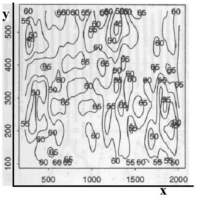
Figure 6: Level lines of fiber volume fraction.

These examples demonstrate how homogenized coefficients can be used in the construction of the optimal shape functions. Of course the question of the “best” choice of homogenized coefficients which lead to a reasonable approximation for general situations is not clear. Nevertheless one can formally proceed by selecting appropriately sized $\omega^{\ast}$ such that it is large with respect to the features of the heterogeneity but such that the heterogeneity is statistically uniform within it. With this in mind we return to the fiber composite portrayed in Figure 1. Figure 6 is a map of the level lines of the volume fraction taken over a moving window given by the square of side length 116 $\mu m$, [2]. It provides a characterization of the spatial variability of the material. The volume fraction varies between 45% and 65% across the sample and clearly demonstrates the statistical inhomogeneity of the material. The correlation between volume fraction and effective elastic properties for this sample is illustrated in Figures 34 and 35 of [2]. These Figures shows that the spatial variation in effective properties correlates well with the variation in volume fraction. With this in mind it appears that we should likely choose $\omega^{*}$ to be of the size 200 $\mu m$.

We conclude this section by considering a periodic heterogeneous medium of fixed period length given by $\epsilon=1/\ell>0$ where $\ell$ is a fixed positive integer. Here we introduce a method for approximation that is derived from the optimal basis associated with the homogenized coefficient obtained from periodic homogenization. In what follows we will denote any constant that is independent of $\epsilon$ and $n$ by $C$. We write the coefficient describing the periodic medium $A^{\epsilon}(x)$ as a rescaling of the coefficient of a unit periodic medium, i.e., $A^{\epsilon}(x)=A(x/\epsilon)$ where $A(y)$ is a coefficient of period one for $y\in\mathbb{R}^{3}$. We denote the unit period cell by $Q$ and the homogenized coefficient $A^{0}$ is given in terms of the periodic corrector matrix $P(y)$, $P_{ij}(y)=\partial_{j}w(y)^{i}+\delta_{ij}$ where $\chi(y)=(w^{1},w^{2},w^{3})$ is the $Q$ periodic solution of

$$divA(y)(\nabla\chi(y)+I)=0,\hbox{for y in Q},$$ (6.7)

and

$$A^{0}=\int_{Q}P(y)dy.$$ (6.8)

The optimal basis for $A^{\epsilon}$ is given in terms of the eigenfunctions $\varphi^{\epsilon}_{i}$ of (5.6). The optimal basis for the homogenized coefficient with $A^{0}$ is given in terms of the eigenfunctions $\varphi^{0}_{i}$ of (5.9). We fix $\epsilon=1/\ell>0$ and the optimal approximation space is given by the span of the restriction of the functions $\varphi^{\epsilon}_{i}$, $i=1,\ldots,n$ to $\omega$. In this implementation we introduce the functions $\phi_{i}^{\epsilon}\in H_{A^{\epsilon}}(\omega^{*})/\mathbb{R}$ such that $\phi_{i}^{\epsilon}=\varphi_{i}^{0}$ on $\partial\omega^{*}$, for $i=1,\ldots,n$. As before we define the approximation space $V_{\epsilon}^{n}(\omega)$ by

$$V_{\epsilon}^{n}(\omega)=span\left\{u^{\epsilon}_{i}=P\phi_{i}^{\epsilon},\,\,\,i=1,\ldots,n\right\}$$ (6.9)

and state the following approximation theorem.

Theorem 6.3.

Given any function $u\in H_{A^{\epsilon}}(\omega^{*})/\mathbf{R}$ then

$$\min_{w\in V_{\epsilon}^{n}(\omega)}\left\{\|u-w\|_{\mathcal{E_{\epsilon}}(\omega)}\right\}\leq(d_{n-1}^{\epsilon}+C\,\epsilon)\|u\|_{\mathcal{E_{\epsilon}}(\omega^{*})},$$ (6.10)

where $d_{n-1}^{\epsilon}$ is the $n$-width associated with $A^{\epsilon}$. Moreover $d_{n-1}^{\epsilon}$ is estimated in terms of an easily computable quantity

$$Q_{\epsilon}^{n}=\sqrt{\int_{\omega}A^{\epsilon}\nabla u^{\epsilon}_{n}\cdot\nabla u^{\epsilon}_{n}\,dx}$$ (6.11)

and the estimate is given by

$$|Q_{\epsilon}^{n}-d_{n-1}^{\epsilon}|\leq\,C\epsilon^{1/2}.$$ (6.12)

Proof. The theorem is proved by constructing upper bounds on the quantity

$$R_{\ell}=\sup_{\{u\in H_{A^{\epsilon}};\,\|u\|_{\mathcal{E}_{\epsilon}(\omega^{*})}=1\}}\left\{\inf_{w\in V^{n}(\omega)}\|u-w\|_{\mathcal{E}_{\epsilon}(\omega)}\right\}.$$ (6.13)

From the corrector theory of periodic homogenization it follows from [27] that there exists a constant $C$ depending only on $\|D^{2}\varphi_{i}^{0}\|_{L^{2}(\omega^{*})}$ and $\alpha<\beta$ for which

$$\|\varphi^{\epsilon}_{i}-\varphi^{0}_{i}\|_{L^{2}(\omega^{*})}\leq\,C\epsilon,$$ (6.14)

and since $\phi_{i}^{\epsilon}\in H_{A^{\epsilon}}(\omega^{*})/\mathbb{R}$ with $A^{\epsilon}$ G-converging to $A^{H}$ and $\phi_{i}^{\epsilon}\rightharpoonup\varphi^{0}_{i}$ it follows again from [27] that

$$\|\phi^{\epsilon}_{i}-\varphi^{0}_{i}\|_{L^{2}(\omega^{*})}\leq\,C\epsilon.$$ (6.15)

Hence

$$\|\varphi^{\epsilon}_{i}-\phi^{\epsilon}_{i}\|_{L^{2}(\omega^{*})}\leq\,C\epsilon.$$ (6.16)

Now consider $u\in H_{A^{\epsilon}}(\omega^{*})/\mathbb{R}$ with $\|u\|_{\mathcal{E}_{\epsilon}(\omega^{*})}=1$. For $w\in V_{\epsilon}^{n}(\omega)$ there are constants $c_{1},c_{2},\ldots,c_{n}$ such that we can write $w=\sum_{i=1}^{n}c_{i}u_{i}^{\epsilon}$ and we choose these constants $c_{1},c_{2},\ldots,c_{n}$ such that $\varphi^{\epsilon}=\sum_{i=1}^{n}c_{i}\varphi_{i}^{\epsilon}$ gives the optimal approximation to $u$ in the $\mathcal{E}_{\epsilon}(\omega)$ norm. For this choice one has

$$\|u-w\|_{\mathcal{E}_{\epsilon}(\omega)} \leq \|u-\sum_{i=1}^{n}c_{i}\varphi_{i}^{\epsilon}\|_{\mathcal{E}_{\epsilon}(\omega)}$$ (6.17)

$$+ \|\sum_{i=1}^{n}c_{i}(\varphi_{i}^{\epsilon}-\phi^{\epsilon})\|_{\mathcal{E}_{\epsilon}(\omega)}$$

$$\leq d_{n-1}^{\epsilon}+\,C\epsilon,$$

where the first term on the last line of the inequality follows from the definition of $n$-width and optimal basis and the second term follows from (6.16) and it follows that $R_{\ell}\leq d_{n-1}^{\epsilon}+C\epsilon$.

We conclude the proof by establishing (6.12). From Theorem 3.1

$$(d_{n-1}^{\epsilon})^{2}=\int_{\omega}A^{\epsilon}\nabla\varphi_{n}^{\epsilon}\cdot\nabla\varphi_{n}^{\epsilon}\,dx,$$ (6.18)

where we have taken the normalization

$$\int_{\omega^{*}}A^{\epsilon}\nabla\varphi_{n}^{\epsilon}\cdot\nabla\varphi_{n}^{\epsilon}\,dx=1.$$ (6.19)

On choosing $u_{n}^{\epsilon}\in V_{\epsilon}^{n}(\omega)$ we write

$$(Q_{\epsilon}^{n})^{2}=\int_{\omega}A^{\epsilon}\nabla u_{n}^{\epsilon}\cdot\nabla u_{n}^{\epsilon}\,dx$$ (6.20)

and

$$(Q_{\epsilon}^{n})^{2}-(d_{n-1}^{\epsilon})^{2}=\int_{\omega}A^{\epsilon}(\nabla u_{n}^{\epsilon}+\nabla\varphi_{n}^{\epsilon})\cdot(\nabla u_{n}^{\epsilon}-\nabla\varphi_{n}^{\epsilon})\,dx.$$ (6.21)

Apriori elliptic estimates show that $C=\sup_{\epsilon>0}\{\|u_{n}^{\epsilon}+\varphi_{n}^{\epsilon}\|_{\mathcal{E}_{\epsilon}(\omega^{*})}\}<\infty$ and

$$|(Q_{\epsilon}^{n})^{2}-(d_{n-1}^{\epsilon})^{2}| \leq C\sqrt{\int_{\omega}A^{\epsilon}(\nabla u_{n}^{\epsilon}-\nabla\varphi_{n}^{\epsilon})\cdot(\nabla u_{n}^{\epsilon}-\nabla\varphi_{n}^{\epsilon})\,dx}$$ (6.22)

$$\leq C\,\|\phi_{n}^{\epsilon}-\varphi_{n}^{\epsilon}\|_{L^{2}(\omega^{*})}\leq\,C\epsilon$$

where the second to last inequality follows from Theorem 3.1 and the last inequality follows from (6.16). Inequality (6.12) follows noting that

$$|Q_{\epsilon}^{n}-d_{n-1}^{\epsilon}|\leq|(Q_{\epsilon}^{n})^{2}-(d_{n-1}^{\epsilon})^{2}|^{1/2}.$$ (6.23)

Appendix A Appendix

We provide a proof of the Cacciappoli inquality given in Lemma 3.1. We introduce the cut off function $\eta\in C_{0}^{1}(\omega^{\ast})$ such that $0\leq\eta\leq 1$ and $\eta=1$ for points inside $\mathcal{O}$ and $|\nabla\eta(x)|\leq 1/\delta$ for points in $\omega^{\ast}$. Given the function $u\in\mathcal{H}(\omega^{\ast})$ and since $u$ is A – harmonic we have

$$\int_{\omega^{\ast}}\,A\nabla u\cdot\nabla(\eta^{2}u)\,dx=0.$$ (A.1)

Expanding (A.1) gives

$$\int_{\omega^{\ast}}\,(A\nabla u\cdot\nabla u)\eta^{2}\,dx=-2\int_{\omega^{\ast}}\,(\eta A^{1/2}\nabla u)\cdot(uA^{1/2}\nabla\eta)\,dx$$

$$\leq 2\left(\int_{\omega^{\ast}}\,(A\nabla u\cdot\nabla u)\eta^{2}\,dx\right)^{1/2}\left(\int_{\omega^{\ast}}\,(A\nabla\eta\cdot\nabla\eta)u^{2}\,dx\right)^{1/2}$$ (A.2)

so

$$\|u\|_{\mathcal{E}(\mathcal{O})}\leq\left(\int_{\omega^{\ast}}\,(A\nabla u\cdot\nabla u)\eta^{2}\,dx\right)^{1/2}\leq 2\left(\int_{\omega^{\ast}}\,(A\nabla\eta\cdot\nabla\eta)u^{2}\,dx\right)^{1/2}$$

$$\leq 2\gamma_{2}\left(\int_{\omega^{\ast}}\,|\nabla\eta|^{2}u^{2}\,dx\right)^{1/2}\leq\frac{2\gamma_{2}^{1/2}}{\delta}\|u\|_{L^{2}(\omega^{\ast})}.$$ (A.3)

and Lemma 3.1 is proved.

We now show that the restriction operators introduced in section three are compact. We first consider two concentric cubes $\omega\subset\omega^{\ast}$. The restriction operator $P:H_{A}(\omega^{*})/\mathbb{R}\rightarrow H_{A}(\omega)/\mathbb{R}$ is defined by $Pu(x)=u(x)$ for all $x\in\omega$ and all $u\in H_{A}(\omega^{*})$.

Lemma A.1.

Given any sequence $\{u_{n}\}_{n=1}^{\infty}\in H_{A}(\omega^{*})/\mathbb{R}$ that is bounded in the energy norm over $(\omega^{*})$ then one can extract a subsequence that converges in $H^{1}(\omega)$ to an element of $H_{A}(\omega)/\mathbb{R}$.

Proof. We apply the Poincare inequality together with the Rellich compactness theorem to extract a convergent subsequence in $L^{2}(\omega^{*})$. From Lemma 3.1 it now follows that this subsequence is Cauchy with respect to the energy norm over $\omega$ and the convergence in $H^{1}(\omega)$ follows. The weak formulation of the boundary value problem together with the strong convergence of the subsequence easily shows that the limit function is $A$-harmonic and the theorem is proved.

Next we consider two concentric cubes $C\subset\omega^{*}$ such that $\omega=C\cap\Omega$ and $\omega^{*}\cap\Omega$ have non zero volume. Here the side length of $C$ is $\sigma$ and that of $\omega^{*}$ is $\sigma^{*}=(1+\rho)\sigma$. The restriction operator $P:H_{A,0}(\omega^{*}\cap\Omega)/\mathbb{R}\rightarrow H_{A,0}(\omega)/\mathbb{R}$ is defined by $Pu(x)=u(x)$ for all $x\in\omega$ and all $u\in H_{A,0}(\omega^{*}\cap\Omega)$. Here we suppose the boundary of $\Omega$ is $C^{1}$.

Lemma A.2.

Given any sequence $\{u_{n}\}_{n=1}^{\infty}\in H_{A,0}(\omega^{*}\cap\Omega)/\mathbb{R}$ that is bounded with respect to the energy norm $(\omega^{*}\cap\Omega)$ then one can extract a subsequence that converges in $H^{1}(\omega)$ to an element of $H_{A,0}(\omega)/\mathbb{R}$.

Proof. Following section 3 we extend each $u_{n}\in H^{1}_{A,0}(\omega^{*}\cap\Omega)/\mathbb{R}$ as an $A$-harmonic function across $\partial\Omega$ onto the set $\omega_{E}^{*}$ such that

$$\|u_{n}\|_{H^{1}(\omega_{E}^{*})}\leq C\|u_{n}\|_{H^{1}(\omega^{*}\cap\Omega)}$$ (A.4)

where $C$ depends only on $\partial\Omega$. Application of Theorem 3.1 gives

$$\|u_{n}\|_{\mathcal{E}(\omega)}\leq\frac{4\beta^{1/2}}{\sigma\rho}\|u_{n}\|_{L^{2}(\omega_{E}^{*})}$$ (A.5)

and we deduce that

$$\|u_{n}\|_{\mathcal{E}(\omega)}\leq C\frac{4\beta^{1/2}}{\sigma\rho}\|u_{n}\|_{L^{2}(\omega^{*}\cap\Omega)}.$$ (A.6)

With (A.6) in hand we can now proceed as in the proof of Lemma A.1 to establish compactness.

References

[1] T. Arbogast and K. J. Boyd. Subgrid upscaling and mixed
multiscale finite elements. SIAM J. Numer. Anal., 44, (2006), 1150–1171.
[2] I. Babuska, B. Anderson, P. Smith and K. Levin, Damage
analysis of fiber composites, Part I Statistical analysis on fiber scale,
Comp. Methods in Appl. Mech and Engrg. 172, (1999), 27-77.
[3] I. Babuska, U. Banerjee and J. Osborn, Generalized Finite
Element Methods–Main Ideas, Results and Perspective, Internat. Journal on
Computational Methods, 1, (2004), 67-103.
[4] I. Babuska and J. Melenk, The Partition of Unity Finite
Element Method, Internat. J. Numerical Methods in Engineering, 40, (1997),
727-758.
[5] I. Babuska, G. Caloz and J. E. Osborn, Special finite element
methods for a class of second order elliptic problems with rough
coefficients, SIAM J. Numer. Anal. 31, (1994), 945–981.
[6] L. Berlyand and H. Owhadi. Flux norm approach to finite dimensional homogenization
approximations with nonseparated length scales and high contrast. Arch. Rat. Mech. Anal., 198, (2010), 177–221.
[7] A. Besounssan, J. L. Lions and G. C. Papanicolau, Asymptotic
Analysis for Periodic Structures, North Holland Pub., Amsterdam 1978.
[8] Weinan E, B. Engquist, X. Li, W. Ren, and E.
Vanden-Eijnden. Heterogeneous multiscale methods: a review. Commun. Comput.
Phys., 2, (2007), 367– 450.
[9] Weinan E, P. Ming, and P. Zhang. Analysis of the
heterogeneous multiscale method for elliptic homogenization problems. J.
Amer. Math. Soc., 18, (2005), 121–156.
[10] Y. Efendiev, V. Ginting, T. Hou, and R. Ewing. Accurate
multiscale finite element methods for two-phase flow simulations. J. Comput.
Phys., 220, (2006), 155–174.
[11] Y. Efendiev and T. Hou. Multiscale finite element
methods for porous media flows and their applications. Appl. Numer. Math.,
57, (2007), 577–596.
[12] B. Engquist and P. E. Souganidis. Asymptotic and numerical
homogenization. Acta Numerica, 17, (2008), 147–190.
[13] T. Y. Hou and Xiao-Hui Wu. A multiscale finite element
method for elliptic problems in composite materials and porous media. J.
Comput. Phys., 134 (1997), 169– 189.
[14] T. Y. Hou, Xiao-Hui Wu, and Yu Zhang. Removing the cell
resonance error in the multiscale finite element method via a
Petrov-Galerkin formulation. Commun. Math. Sci., 2 (2004), 185–205.
[15] J. M. Melenk, On –widths for elliptic problems. Journal
of Mathematical Analysis and Applications 247, (2000), 272–289.
[16] N. Meyers, An –Estimate for the gradient of solutions
of second order elliptic divergence equations. Annali della Scuola Norm.
Sup. Pisa 17 (1963), 189–206.
[17] F. Murat, H-convergence, Séminaire d’Analyse Fonctionelle et Numérique de l’Université d’Alger, mimeographed notes (1978). L.
Tartar Cours Peccot, College de France (1977). Translated into English as F.
Murat L. Tartar, H- convergence, in Topics in the Mathematical Modeling of
Composite Materials (ed. A. V. Cherkaev R. V. Kohn), pp. 21–43,
Progress in Nonlinear Differential Equations and their Applications, Vol. 31, Birkhäuser, Boston.
[18] J. Nolen, G. Papanicolaou, and O. Pironneau. A framework for
adaptive multiscale methods for elliptic problems. Multiscale Model. Simul.,
7, (2008), 171–196.
[19] H. Owhadi and L. Zhang. Metric-based upscaling. Comm.
Pure Appl. Math., 60, (2007), 675–723.
[20] H. Owhadi and L. Zhang. Homogenization of parabolic
equations with a continuum of space and time scales. SIAM J. Numer. Anal.,
46, (2007), 1–36.
[21] B. N. Parlett, The Symmetric Eigenvalue Problem, SIAM, 1998.
[22] A. Pinkus, –Widths in Approximation Theory.
Springer–Verlag, Berlin, Heidelberg, New York, 1985.
[23] S. Spagnolo, Convergence in Energy for Elliptic Operators, in :
B. Hubbard ( Ed.) Numerical Solutions of Partial Differential Equations III,
( Synspade 1975, College Park, Maryland,1975), Academic Press, New
York,(1975).
[24] T. Strouboulis, L. Zhang and I Babuska, Assessment of the cost
and accuracy of Generalized FEM. Internat. J. Numerical Methods in
Engineering, 69, (2007), 250-283.
[25] T. Strouboulis, I. Babuska, and K. Copps, The design and
analysis of the generalized finite element method , Comp. Methods in Appl.
Mech. and Engrg., 181, (2001), 43-69.
[26] T. Strouboulis, L. Zhang, and I. Babuska, p-version of
generalized FEM using mesh based handbooks with applications to multiscale
problems Int. J. Num. Meth. Engrg., 60, (2004), 1639-1672.
[27] V. V. Zhikov, S. M. Kozlov, and O. A. Oleinik, Homogenization
of Differential Operators and Integral Functionals. Springer-Verlag, Berlin,
New York, 1994.
[28] Hermann Weyl. Über gewöhnliche Differentialgleichungen mit Singularitäten und die zugehörigen Entwicklungen
willkürlicher Funktionen. Math. Ann., 68, (1910), 220– 269.