UT-10-05

IPMU10-0067

NSF-KITP-10-041

More on Dimension-4 Proton Decay Problem in F-theory

— Spectral Surface, Discriminant Locus and Monodromy —

Hirotaka Hayashi¹, Teruhiko Kawano¹, Yoichi Tsuchiya¹ and Taizan Watari²

¹Department of Physics, University of Tokyo, Tokyo 113-0033, Japan

²Institute for the Physics and Mathematics of the Universe, University of Tokyo, Kashiwano-ha 5-1-5, 277-8583, Japan

1 Introduction

Considerable progress has been made in the last two years in understanding flavor structure in F-theory compactifications. Supersymmetric compactifications of F-theory to 3+1 dimensional space-time is described primarily by a set of data $(X_{4},G^{(4)})$, where $X_{4}$ is an elliptic fibered Calabi–Yau 4-fold and $G^{(4)}$ a 4-form flux on it. Non-Abelian gauge theories like SU(5)_GUT unified theories can arise from singular geometry of $X_{4}$. It is difficult to extract physics directly from singular geometry, but low-energy effective theory associated with the singular local geometry of $X_{4}$ can be described by using non-Abelian gauge theory in 7+1 dimensions [1] to some level of approximation. It has been the key in the progress in the understanding of flavor structure in F-theory to use this gauge-theory effective description [2, 3]. See also [4, 5, 6, 7, 8, 9].

In supersymmetric compactification for realistic models, dimension-4 proton decay operators

$$\Delta W\ni\bar{\bf 5}_{M}\cdot{\bf 10}\cdot\bar{\bf 5}_{M}$$ (1)

have to be brought under control. An obvious solution is

• to consider a compactification with $(X_{4},G^{(4)})$ that has a $\mathbb{Z}_{2}$ symmetry [6].

The $\mathbb{Z}_{2}$ symmetry will become an $R$-parity (or equivalently a matter parity) in the low-energy effective theory below the Kaluza–Klein scale. Other solutions to the problem include

• rank-5 GUT scenario, that is, to consider $\mathop{\rm SU}(6)$ or $\mathop{\rm SO}(10)$ GUT models [10],

• factorized spectral surface scenario [6, 11] (see also [12, 13, 14, 15]), and

• spontaneous $R$-parity violation scenario [10, 6] (see also [16]).

The scenario (ii) is a special case of (iii), and is also a special case of (iv).

The factorized spectral surface scenario (iii), however, is not without a theoretical concern [6]. The dimension-4 proton decay problem is so severe that the coupling (1) should be extremely small even if they are present. The question is whether we have a theoretical framework in which the scenario can be formulated rigorously and even an extremely small contribution to (1) can be studied. At least so far, the answer is no. It is, thus, important to study to what extent this scenario works, and that is what we do in this article.

Heart of the idea of the factorized spectral surface scenario is to consider a factorization limit of the spectral surface so that

• matter fields $\bar{\bf 5}_{M}$ and Higgs fields $\bar{\bf 5}_{H}$ are associated with irreducible components of the spectral surface for fields in the $\bar{\bf 5}$ representation of $\mathop{\rm SU}(5)_{\rm GUT}$, and

• an unbroken U(1) symmetry remains in the low-energy effective theory below the Kaluza–Klein scale, and the operator (1) is ruled out because of the symmetry.

This scenario has been formulated by using the gauge theory description in 7+1 dimensions. Because of the approximate nature of the gauge theory description, factorization is not rigorously well-defined; there are also some corrections that have not been captured in the gauge theory description on 7+1 dimensions [6]. We will explain these limitations of the gauge theory description on 7+1 dimensions more in detail in section 2, although these materials have almost been spelled out in [6, 11] (see also [5]).

In section 3, we study monodromy of 2-cycles in $X_{4}$ instead of a gauge theory on 7+1 dimensions, in order to find out whether an unbroken U(1) symmetry remains in the low-energy effective theory. We conclude in section 4 that the proton decay operators (1) are expected to be generated in the factorized spectral surface scenario, but we also list some loopholes in the argument. The appendix A explains calculation of the monodromy of 2-cycles using language of string junction in detail; all the necessary techniques in the appendix A, however, are already available in the literature (e.g., [17]). The monodromy matrices obtained in this way in F-theory language can be understood much more transparently in dual Heterotic language; this is the subject of the appendix B.

2 Effects Beyond Gauge Theory in 7+1 Dimension

The gauge theory description on 7+1 dimensions in F-theory captures geometry of a local neighbourhood of a discriminant locus of an elliptic fibration [1]. When a geometry of an elliptically fibered Calabi–Yau 4-fold $\pi_{X}:X_{4}\rightarrow B_{3}$ is locally approximately an ALE space of A–D–E type in the direction transverse to the discriminant locus, gauge theory of the same A–D–E type describes the physics associated with this local geometry. Thus, by construction, the gauge theory description has limited power in capturing the physics of geometry in the transverse direction; only physics associated with non-compact (local) geometry that is approximately ALE fibration can be captured approximately. When it comes to the dimension-4 proton decay problem, this approximate nature of the gauge theory description of F-theory can be a problem.

To see this more explicitly, let us consider a local geometry given by the generalized Weierstrass form

$$y^{2} = x^{3}-A_{1}yx+A_{2}x^{2}-A_{3}y+A_{4}x+A_{6},$$ (2)

where $(x,y)$ are coordinates of the elliptic fiber of $X_{4}$, and $A_{1,\cdots,4,6}$ are regarded as functions locally on $B_{3}$. For an ${\rm SU}(5)_{\rm GUT}$ GUT model [18], we need to consider a case where $A_{1,\cdots,4,6}$ are in the form of

$$A_{k}=(-)^{k}\left[z^{k-1}a_{6-k}+z^{k}a^{\prime}_{6-k}+z^{k+1}a^{\prime\prime}_{6-k}+\cdots\right],$$ (3)

where $z$ is a local coordinate of a base manifold $B_{3}$; the $z=0$ locus becomes an irreducible component $S_{GUT}$ of the discriminant locus $\Delta$. $a_{0,2,3,4,5}$ and $a^{\prime}_{0,2,3,4,5}$ are coefficients that depend on two local coordinates on $S_{GUT}$. Consider, for example, a case, when all of $a_{2,3,4,5}$ are small in a way indicated by

$$a_{5}=\epsilon_{K}^{5}a_{5,*},\;\;a_{4}=\epsilon_{K}^{4}a_{4,*},\;\;a_{3}=\epsilon_{K}^{3}a_{3,*},\;\;a_{2}=\epsilon_{K}^{2}a_{2,*}$$ (5)

for $a_{5,*}$, $a_{4,*}$, $a_{3,*}$, $a_{2,*}$ of all $\sim{\cal O}(1)$. $\epsilon_{K}$ is a small parameter that is different from zero. We know that this geometry nearly has an $E_{8}$ singularity around $z=0$; to be more precise, there are four vanishing 2-cycles right at $z=0$, and there are four small 2-cycles near $z=0$. One can focus on the geometry of these small 2-cycles by choosing a new set of coordinates $(x^{\prime},y^{\prime},z^{\prime})$:

$$x=\epsilon_{K}^{10}x^{\prime},\;\;y=\epsilon_{K}^{15}y^{\prime},\;\;z=\epsilon_{K}^{6}z^{\prime}.$$ (6)

With these new coordinates and coefficients $a_{r,*}\sim{\cal O}(1)$ ($r=0,2,3,4,5$), the local defining equation (2) becomes exactly the $E_{8}$ singularity with relevant deformation parameters [19], with correction terms whose coefficients are suppressed by positive power of the small number $\epsilon_{K}$. The gauge theory description focuses on the geometry of these small 2-cycles (i.e., forgets about the rest of the geometry), and further make an approximation of ignoring the correction terms that are small but present [4] (see also [5, 11]). Even when the $\epsilon_{K}$ scaling of the coefficients is assumed as above to maximize the number of small 2-cycles captured in a gauge theory description, the gauge theory description is only an approximate description of the compact geometry $X_{4}$ by construction [6]. Let us call this Problem A.

We may have another difficulty in justifying the factorized spectral surface scenario in the gauge theory description. To see this, let us remind ourselves of the following. Since $\bar{\bf 5}_{M}$ and $\bar{\bf 5}_{H}$ multiplets are zero modes appearing in the low-energy effective theory below the Kaluza–Klein scale, the factorization of the spectral surface should be defined globally on the GUT divisor $S_{GUT}$. Field theory local model in an open patch $U_{a}\subset S_{GUT}$, on the other hand, captures very small 2-cycles in the ALE fiber in addition to the four vanishing 2-cycles in $A_{4}$ singularity, and hence the rank of gauge group in $U_{a}$ may be different from the rank in another open patch $U_{b}\subset S_{GUT}$ [1, 3, 13, 4]; these local descriptions with gauge groups of varying rank are glued together approximately in overlapping regions of open patches $\{U_{a}\}_{a\in A}$ to cover the entire ALE-fibered geometry over $S_{GUT}$. The global factorization of the spectral surface, however, cannot be well-defined, when the rank of the spectral surface varies from one patch to another. This problem can be avoided if we consider a Higgs bundle that has a fixed rank over the entire $S_{GUT}$.

Fixed rank Higgs bundle description over the entire $S_{GUT}$, however, often breaks down somewhere in $S_{GUT}$. For example, a rank-$k$ spectral surface $C$ is defined globally in $K_{S}$ by

$$a_{5-k}\xi^{k}+\cdots+a_{4}\xi+a_{5}=0,$$ (7)

where $\xi$ is the fiber coordinate of the canonical bundle $\pi_{K_{S}}:K_{S}\rightarrow S$, if $a_{r}$’s ($5-k\leq r\leq 5$) are global holomorphic sections of line bundles ${\cal O}(rK_{S}+\eta)$ for some divisor $\eta$ in $S_{GUT}$. $\pi_{K_{S}}|_{C}:C\rightarrow S$ is an $k$-fold cover at generic points of $S_{GUT}$, but when the coefficient of the highest degree term $a_{5-k}$ vanishes, one of the $k$ solutions of (7) shoots off to infinity in the fiber direction of $\pi_{K_{S}}:K_{S}\rightarrow S_{GUT}$. This behavior of the spectral surface indicates that one of (very) small 2-cycles becomes relatively large there. It is not a sensible approximation to keep the physics associated with all the 2-cycles in (7) while ignoring all others in a local neighbourhood around the zero locus of $a_{5-k}$ . As long as the divisor $(5-k)K_{S}+\eta$ is effective, this does happen somewhere in $S_{GUT}$. The problem in this neighbourhood can be fixed (c.f. [3]) by adopting a Higgs bundle that is one-rank higher, a rank-$(k+1)$ Higgs bundle, as long as $a_{4-k}$ is not identically zero. We still encounter the same problem around the zero locus of $a_{4-k}$. One could still crank the rank of gauge group up, once again. But $E_{8}$ gauge group is maximal in the E series of the A–D–E classification, and we come to a dead end.

We could consider a Calabi–Yau 4-fold $X_{4}$ for F-theory compactification which is approximately an ALE fibration of $E_{8}$ type over $S_{GUT}$ in the neighbourhood along $S_{GUT}$. This is done by choosing the coefficients indicated as in (5) [5]. When we take GUT gauge group as SU(5)_GUT, we have a 5-fold spectral cover,

$$a_{0}\xi^{5}+a_{2}\xi^{3}+a_{3}\xi^{2}+a_{4}\xi+a_{5}=0.$$ (8)

Factorization conditions can be imposed on (8) in an $E_{8}$ gauge theory defined globally on $S_{GUT}$ [11]. That is the best we hope to do within gauge theories on 7+1 dimensions. In a region of $S_{GUT}$ around a point where $a_{0}$ vanishes, however, two roots of (8) become large, as

$$\xi\sim\pm i\sqrt{(a_{2}/a_{0})}.$$ (9)

The $E_{8}$ gauge theory is not a sensible approximation in the local neighbourhood of the $a_{0}=0$ locus, because the corresponding two 2-cycles are no longer relatively small. In a region slightly away from the $a_{0}=0$ locus, one can see that the two roots (and hence the Higgs field vevs $\varphi$ in two diagonal entries) are exchanged when the phase of $a_{0}$ changes by $2\pi$. This phenomenon indicates that the two 2-cycles not just become large, but also are twisted by a monodromy around the $a_{0}=0$ locus. 2-cycles that are not captured by the $E_{8}$ gauge theory may also be involved in this monodromy, because there is no clear separation between the 2-cycles within $E_{8}$ and those that are not around the $a_{0}=0$ locus. In order to study geometry and physical consequences associated with this behavior, one has to go beyond $E_{8}$ gauge theory on 7+1 dimensions. We call this Problem B.

Clearly we need a theoretical idea how to study whether the operator (1) is generated or not; a new idea should keep the successful aspects of the factorized spectral surface scenario, while it should not rely on the gauge theory descriptions in 7+1 dimensions. While spectral surfaces can be defined only within the gauge theory descriptions, the essence of the scenario is to keep an unbroken U(1) symmetry in the low-energy effective theory below the Kaluza–Klein scale. We can thus focus on a question whether an unbroken U(1) symmetry is maintained (or how to find one) in F-theory compactifications. Noting that topological 2-forms of certain type in $X_{4}$ yield U(1) vector fields in 3+1 dimensions [20, 21], and that the vector fields are always accompanied by U(1) symmetries, we see that a solution is to focus on geometry of $X_{4}$, instead of gauge theory associated with the canonical bundle $K_{S}$ on $S_{GUT}$.

Since we are interested in U(1) symmetries under which $\mathop{\rm SU}(5)_{\rm GUT}$-charged matter fields on $S_{GUT}$ are charged, we are interested in 2-forms of $X_{4}$ which have components dual to 2-cycles in the local ALE fiber approximation along $S_{GUT}$ in $X_{4}$. It is a topological problem whether or not an extra U(1) symmetry remains unbroken. We keep tracks of topological 2-forms / 2-cycles to address this problem; it is not necessary to restrict our attention only to 2-cycles contained in one of the $A$–$D$–$E$ types, or to 2-cycles that are relatively small. All the 2-cycles in $X_{4}$ can be treated in an equal footing, and hence, we are free from all the problems in the gauge theory description on 7+1 dimensions. The factorization condition of the spectral surface for an unbroken U(1) symmetry is replaced by a condition that there is at least one monodromy-invariant 2-cycle over $S_{GUT}$.

3 Monodromy of 2-Cycles

In this section, we study monodromy of 2-cycles in a Calabi–Yau 4-fold $X_{4}$ and discuss whether an unbroken U(1) symmetry remains or not when the spectral surface satisfies a factorization condition. In section 3.2, we show that certain subgroup of the monodromy corresponds to what we expect from the gauge theory descriptions on 7+1 dimensions. This subgroup reduces to a smaller one when the spectral surface is in the factorization limit, and there is a monodromy invariant 2-cycle [and hence an unbroken U(1)] at this level of analysis. This guarantees that we can keep the heart of the idea of the factorized spectral surface scenario without relying on the gauge theory description. Section 3.3 explains the structure of the full monodromy group; the subgroup in section 3.2 is a proper subgroup of the full monodromy group. We study monodromy of 2-cycles for some other generators in section 3.4, and find that there is no monodromy-invariant 2-cycles when the full monodromy group is taken into consideration. This means that there is no unbroken U(1) symmetry in the effective theory in the factorized limit of the spectral surface.

3.1 The model and the notation

In the study of monodromy of 2-cycles in sections 3.2–3.4, we only consider a special case where a Calabi–Yau 4-fold $X_{4}$ is a K3 fibration over $S_{GUT}$: $\pi^{\prime}_{X}:X_{4}\rightarrow S_{GUT}$. One of the advantages of this $X_{4}$ as a global fibration on $S_{GUT}$ is that the U(1) vector fields in 3+1 dimensions, and hence the non-$H^{2}(B_{3})$ non-$H^{0}(B_{3};R^{2}\pi_{X*}\mathbb{Z})$ components of $H^{2}(X_{4};\mathbb{Z})$ can be studied by $H^{0}(S_{GUT};R^{2}\pi^{\prime}_{X*}\mathbb{Z})$ [23, 2, 24]. Global sections of the local system $R^{2}\pi^{\prime}_{X*}\mathbb{Z}$ correspond precisely to the monodromy invariant 2-cycles in the fiber of $\pi^{\prime}_{X}:X_{4}\rightarrow S_{GUT}$, and hence the problem can be formulated as a local theory on 7+1 dimensions (if not as a local gauge theory on 7+1 dimensions). Although this advantage may appear to be available only for a special case, global fibration of $X_{4}$ over $S_{GUT}$, we consider otherwise. Topological 2-cycles in a neighbourhood of $S_{GUT}$ can be captured by a local system like $R^{2}\pi^{\prime}_{X*}\mathbb{Z}$ at least locally, if not globally. Since the monodromy among 2-cycles is about a non-trivial local behavior of such a local system at special points (which we call monodromy locus later in this article), one only has to examine local behavior of such local systems to find out whether a U(1) symmetry is projected out or not. Thus, although the following presentation in this section may appear to rely exclusively on a $X_{4}$ that is a global fibration on $S_{GUT}$, we do not loose generality as a study of F-theory compactifications. Discussion on non-K3 fibered cases is found in section 3.5.

The other advantage is that we know a lot about 2-cycles of K3 manifold, so that we can make our presentation very concrete. Since the monodromy around $a_{0}=0$ locus might involve not just 2-cycles within $E_{8}$ but also other 2-cycles in the direction transverse to the GUT divisor $S_{GUT}$, we certainly need a geometry for analysis where such an “other 2-cycle” is identified. With a compact K3 manifold in the transverse direction, we have all the necessary techniques. On the other hand, we do not loose generality by this specific choice, because we are interested only in the local behavior of monodromy among 2-cycles in $E_{8}$ and those that are “adjacent” to them.

In principle, we could study monodromy of 2-cycles in a configuration of real interest, where the $A_{4}$ singularity is along $S_{GUT}$, and a factorization condition is imposed on the 5-fold spectral cover (8). Instead of this realistic $E_{8}\rightarrow\mathop{\rm SU}(5)_{\rm GUT}$ symmetry breaking model, however, we study monodromy of 2-cycles in an $E_{8}\rightarrow E_{6}$ symmetry breaking model. 2+1 factorization condition can be imposed on the 3-fold spectral cover

$$a_{0}\xi^{3}+a_{2}\xi+a_{3}=0.$$ (10)

Moreover, since the 2-cycles associated with the hidden sector is not essential in our problem, we consider a configuration with an unbroken hidden $E_{8}$ symmetry. Namely, we study monodromy of 2-cycles in $X_{4}$ whose K3 fibration structure is given by

$$y^{2}=x^{3}+(a_{2}z^{3}+f_{0}z^{4})x+\left(\frac{1}{4}a_{3}^{2}z^{4}+a_{0}z^{5}+g_{0}z^{6}+a^{\prime\prime}_{0}z^{7}\right)\,.$$ (11)

Here, $(x,y)$ are coordinates of the elliptic fiber of $X_{4}$, $z$ an inhomogeneous coordinate of the base $\mathbb{P}^{1}$ of K3 and $a_{0,2,3},a^{\prime\prime}_{0},f_{0},g_{0}$ are sections of some line bundles on $S_{GUT}$.

When F-theory is compactified on a K3 manifold that is an elliptic fibration $\pi_{K3}:K3\rightarrow\mathbb{P}^{1}$ with a section, then there are 20 2-cycles dual to $H^{1}(\mathbb{P}^{1};R^{1}\pi_{K3*}\mathbb{Z})$ and corresponding U(1) symmetries in 7+1 dimensions. Such topological 2-cycles can be described by string junctions on the base $\mathbb{P}^{1}$. All the necessary details in how to find independent 20 configuration of such junctions [17] are reviewed in the appendix A.

In order to calculate monodromy of 2-cycles, or equivalently to see how the local system $R^{2}\pi^{\prime}_{X*}\mathbb{Z}$ is twisted, one first has to take a base point $b\in S_{GUT}$, and set a basis in the (co)homology group of $H_{2}(\pi^{{}^{\prime}-1}_{X}(b);\mathbb{Z})\simeq H_{2}({\rm K3};\mathbb{Z})$. For a loop $\gamma$ on $S_{GUT}$ that starts and ends on the base point $b$, we can trace the basis elements $H_{2}(\pi^{{}^{\prime}-1}_{X}(p);\mathbb{Z})$ for points $p$ on the loop $\gamma$, starting from the base point $b$ until we come back to the base point again. The calculation of monodromy is practically carried out by tracing string junction configuration that correspond to the basis elements of $H_{2}(\pi^{{}^{\prime}-1}_{X}(b);\mathbb{Z})$. We only have to trace along the loop $\gamma$ the motion of discriminant locus points—$[p,q]$ 7-branes—in the complex $z$ plane. All the necessary techniques in this monodromy analysis is quite standard in Type IIB string theory. We thus present detailed procedure of practical calculation of monodromy for only three loops in the appendix A; for all other loops, only the results are presented in this article.

It is convenient to introduce a notation for a set of independent 2-cycles of the K3 fiber and also to assign names to individual $[p,q]$ 7-branes at a base point $b$. To the 24 discriminant points, we assign the following names: $A8$–$A1$, $B$, $C1$, $C2$, $D$, $A8^{\prime}$–$A1^{\prime}$, $B^{\prime}$, $C1^{\prime}$, $C2^{\prime}$ and $D^{\prime}$. The appendix A explains the choice of the base point $b$, location of the the 24 7-branes in the $z$ plane, as well as their $[p,q]$ charges for the base point. We assign names (notation) such as $C_{A76}$, $C_{A65}$ etc. to string junction configurations and corresponding 2-cycles of ${\rm K3}=\pi^{{}^{\prime}-1}(b)$. All the details are written in the appendix A, but the most relevant part of the information is summarized in Figure 1.

Figure 1: The independent 2-cycles of a K3 surface. Dotted lines represent the branch cuts of 7-branes. Black blobs represent $A$-branes, open circles are B-branes, open boxes correspond to C-branes and open triangles are “D”-branes whose $[p,q]$ charge is [3, 1]. $A8^{\prime}\sim D^{\prime}$ 7-branes have the same $[p,q]$ charges as those without a ^′, and are ordered from left to right as in the same way as $A8\sim D$ 7-branes. 7-branes from $A7$ to $C2$ and those from $A7^{\prime}$ to $C2^{\prime}$ constitute separate sets of $[A^{7}BC^{2}]$ 7-brane configuration of $E_{8}$.

There is no unique choice of a basis of $H_{2}({\rm K3};\mathbb{Z})$, but one of the most convenient choices is to use the 2-cycles listed in Table 1.

2-cycles inside $E_{8}$	$C_{A76},C_{A65},C_{A54},C_{A43},C_{A32},C_{A21},C_{ABC},C_{C12}$
2-cycles outside $E_{8}$	$C_{\alpha}^{1}$, $C_{\alpha}^{2}$, $C_{\beta}^{1}$, $C_{\beta}^{2}$
those for hidden $E_{8}$	$C^{\prime}_{A76},C^{\prime}_{A65},C^{\prime}_{A54},C^{\prime}_{A43},C^{\prime}_{A32},C^{\prime}_{A21},C^{\prime}_{ABC},C^{\prime}_{C12}$

Table 1: A convenient choice of a basis of $H_{2}(\pi^{{}^{\prime}-1}(b);\mathbb{Z})$.

Among them, $C_{\alpha}^{1,2}$, $C_{\beta}^{2}$ need to be defined by linear combinations of string junction configurations like those in Figure 1; see (99, 100). The intersection form becomes (98). The intersection form within the eight 2-cycles in the first row of Table 1 is described by the Dynkin diagram of $E_{8}$ shown in Figure 2.

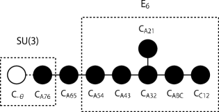
Figure 2: 2-cycles inside $E_{8}$ and their intersection. Note that $C_{-\theta}$ is not the same as $C_{A87}$; see footnote 24 for more.

As we study monodromy of 2-cycles in (11) that has unbroken $E_{6}$ symmetry (split form $E_{6}$ singularity) [18], monodromy matrices must be trivial on a subspace generated purely by $C_{A54},C_{A43},C_{A32},C_{A21},C_{ABC},C_{C12}$, the simple roots of $E_{6}$. Thus, we can choose $C_{-\theta}$ as a basis element instead of $C_{A65}$ as in Table 1, where $C_{-\theta}$ is a linear combination purely of the 2-cycles in the first row of Table 1,

$$C_{-\theta}=-(2C_{A76}+3C_{A65}+4C_{A54}+5C_{A43}+6C_{A32}+4C_{ABC}+3C_{A21}+2C_{C12})\,.$$ (12)

The six 2-cycles of $E_{6}$ and the two 2-cycles $C_{A76}$ and $C_{-\theta}$ for the “structure group” $\mathop{\rm SU}(3)_{\rm str}$ are orthogonal in the intersection form. Since we restrict ourselves in a region of moduli space where the hidden $E_{8}$ 2-cycles do not participate in the monodromy, the monodromy can be represented by $6\times 6$ matrices acting on a vector space generated by $C_{A76},C_{-\theta},C_{\alpha}^{1},C_{\alpha}^{2},C_{\beta}^{1}$ and $C_{\beta}^{2}$.

The calculation of monodromy boils down to following the trace of the $[p,q]$ 7-branes along paths in $S_{GUT}$. Thus, an explicit expressions for the discriminant of (11) is very useful:

$$\Delta=z^{8}\Delta^{\prime}$$ (13)

where $\Delta^{\prime}$ is given by

$$\begin{split}\Delta^{\prime}&=\frac{27}{16}a_{3}^{4}+\left(\frac{27}{2}a_{0}a_{3}^{2}+4a_{2}^{3}\right)z+\left(\frac{27}{2}a_{3}^{2}g_{0}+27a_{0}^{2}+12a_{2}^{2}f_{0}\right)z^{2}\\ &\quad+\left(54a_{0}g_{0}+12a_{2}f_{0}^{2}+\frac{27}{2}a_{3}^{2}a^{\prime\prime}_{0}\right)z^{3}+(4f_{0}^{3}+27g_{0}^{2}+54a_{0}a^{\prime\prime}_{0})z^{4}\\ &\quad+54a^{\prime\prime}_{0}g_{0}z^{5}+27a^{{}^{\prime\prime}2}_{0}z^{6}\,.\end{split}$$ (14)

In this model, eight 7-branes $A5$–$A1$ and $B$, $C1$, $C2$ are at an $E_{6}$ singularity at $z=0$ [25, 26], and ten 7-branes $A7^{\prime}$–$A1^{\prime}$, $B^{\prime}$, $C1^{\prime}$and $C2^{\prime}$ form an $E_{8}$ singularity at $z=\infty$. The six other 7-branes, $A6$, $A7$, $A8$, $D$, $A8^{\prime}$ and $D^{\prime}$, are the zero points of $\Delta^{\prime}$ above. Along a path $\gamma$ in $S_{GUT}$, values of all the coefficients $a_{0,2,3}$, $f_{0}$, $g_{0}$ and $a^{\prime\prime}_{0}$ change, and hence the six 7-branes change their locations in the $z$-plane. We can thus determine the monodromy matrix by following the 7-branes and string junctions.

In sections 3.2–3.4, we present monodromy matrices obtained as a result of such a calculation. Although the monodromy for a loop $\gamma$ in $S_{GUT}$ is ultimately what we are interested in, it is a better idea to study monodromy of 2-cycles in a little more abstract level; we will study monodromy of 2-cycles for loops in a moduli space of an elliptic K3 manifold. Since any loops in $S_{GUT}$ are mapped by the choice of sections $a_{0,2,3}$, $f_{0}$ etc. to loops in the moduli space of the elliptic K3 manifold, the monodromy group for the loops on $S_{GUT}$ is obtained by a pull-back of the monodromy group for the loops on the elliptic K3 moduli space by the sections. Such questions as whether an unbroken U(1) symmetry exists can be answered at the level of monodromy on the elliptic K3 moduli space, independent of specific details of $S_{GUT}$ or sections $a_{0,2,3}$ etc. on it.

3.2 The monodromy in 8D gauge theory region

In the factorization limit of the spectral surface, the monodromy group of 2-cycles captured in the gauge theory description on 7+1 dimensions is reduced; there is no question about this statement in the deformation of $A_{N+M}$ singularity to $A_{M}$. This statement is believed to be true also in deformation of $E_{6,7,8}$ type singularity to $A_{4}$ [4, 6] (see also [2]), for example, but it has not been confirmed directly so far by looking at 2-cycles in $X_{4}$. In this section 3.2, we study explicitly the geometry of 2-cycles in $X_{4}$ when the spectral surface is at the factorization limit, and confirm that the statement above is correct. This justifies our strategy to replace the factorization limit of spectral surfaces by existence of monodromy invariant 2-cycles.

At the same time, we will see that the monodromy of 2-cycles that appear in the gauge theory description on 7+1 dimensions is only a proper subgroup of the entire monodromy group of the whole theory. Thus, it will be clear what one overlooks in the gauge theory description on 7+1 dimensions.

The family of elliptic K3 manifold (11) is parametrized by $(a_{0},a_{2},a_{3},f_{0},g_{0},a^{\prime\prime}_{0})$, among which two are redundant because of the freedom to rescale the coordinates $(x,y,z)$. Instead of using a set of “gauge invariant” parameters of this moduli space such as $(a_{0}a^{\prime\prime}_{0}/g_{0}^{2})$ and $(a_{2}/a_{0})(4f_{0}^{3}+27g_{0}^{2})^{1/6}$, we fix a gauge by fixing the values of $f_{0}$ (or $g_{0}$) and $a^{\prime\prime}_{0}$.

The full scope of the problem is to consider all possible loops in the moduli space of (11) and determine the monodromy of 2-cycles of the K3 for the loops. We restrict our attention in this section, however, to a subset of the moduli space

$$a_{0}=a_{0,*}\epsilon_{\eta},\quad a_{2}=a_{2,*}\epsilon_{K}^{2}\epsilon_{\eta},\quad a_{3}=a_{3,*}\epsilon_{K}^{3}\epsilon_{\eta},$$ (15)

where parameters $a_{r,*}\in\mathbb{C}$ and $g_{0}\in\mathbb{C}$ are at most ${\cal O}(1)$; $0\neq|\epsilon_{K}|\ll 1$ and $0\neq|\epsilon_{\eta}|\ll 1$ are fixed numbers, and we fix the “gauge” by setting $f_{0}=-1$ and $a^{\prime\prime}_{0}=\epsilon_{\eta}$. Because $|\epsilon_{\eta}|\ll 1$, the elliptic K3 manifold is always close to the stable degeneration limit [20, 27] within the subset specified above. We call this subset scaling region. It helps in ensuring the validity of the gauge theory description in 7+1 dimensions, but not quite, to set $\epsilon_{K}$ as a small number. We will see this in detail in the rest of this section in F-theory language. The appendix B will provide a very clear explanation of this in the dual Heterotic language. The base point of the moduli space is chosen within this subset, and only loops that stay within this subset are considered in this section. Although this is only to find part of the monodromy group, we will see that this partial result is interesting enough from mathematical and physical points of view, and is also sufficient in drawing conclusions for practical purposes.

We will call a subset of the scaling region characterized by

$$|\epsilon_{K}|^{2}\ll|a_{0,*}|\sim{\cal O}(1)$$ (16)

as an 8D gauge theory region. We will see in this section 3.2 that all the loops (except the one mentioned at the end of section 3.4) that stay within this “ 8D gauge theory region” yield monodromies of 2-cycles that are expected from the gauge theory descriptions on 7+1 dimensions.

For any points in the 8D gauge theory region of the moduli space, the six 7-branes specified by $\Delta^{\prime}=0$ are distributed in the complex $z$ plane as follows; there are two 7-branes in the region $z\sim{\cal O}(\epsilon_{K}^{6}\epsilon_{\eta})$, two in the region $z\sim{\cal O}(\epsilon_{\eta})$, and two in $z\sim{\cal O}(\epsilon_{\eta}^{-1})$. These three groups of 7-branes remain distinct along any loops that stay within the 8D gauge theory region of the moduli space. It is, thus, appropriate to identify that the two 7-branes in the ${\cal O}(\epsilon_{\eta}^{-1})$ region as the 7-branes $A8^{\prime}$ and $D^{\prime}$, those in the ${\cal O}(\epsilon_{\eta})$ region as $A8$ and $D$, and those in the ${\cal O}(\epsilon_{K}^{6}\epsilon_{\eta})$ region as $A6$ and $A7$, respectively. Over the entire 8D gauge theory region, the positions of the 7-branes A6, A7 are effectively given by the zero points of

$$\Delta^{\prime}_{\mathrm{lower-quadr}}=\frac{27}{16}a_{3}^{4}+\left(\frac{27}{2}a_{0}a_{3}^{2}+4a_{2}^{3}\right)z+27a_{0}^{2}z^{2}\,,$$ (17)

which is approximately the first three terms of the right hand side of (14).

The string junction configuration (and the corresponding 2-cycles) $C_{A76}$ and $C_{-\theta}$ correspond to the two roots of $\mathop{\rm SU}(3)_{\rm str}$, the commutant of $E_{6}$ within $E_{8}$. As a point moves along a loop in (the 8D gauge theory region of) the moduli space, the coefficients $a_{0,2,3}$ in (17) change, and the positions of the $A7$ and $A6$ 7-branes move in the complex $z$-plane. Consequently the branch cuts and the string junction configurations also have to change continuously. Monodromy of the two 2-cycles $C_{A76}$ and $C_{-\theta}$ should reproduce what we expect from the 8D gauge theory descriptions.

Such loops in the moduli space should avoid a locus where more than one 7-branes come on top of one another, because the elliptic K3 “manifold” becomes singular and it is subtle to talk of “topological 2-cycles” there. The degeneration of the A6 and A7 7-brane positions are characterized by the discriminant locus of the quadratic equation $\Delta^{\prime}_{\mathrm{lower-quadr}}=0$:

$$\tilde{\Delta}_{\mathrm{lower-quadr}}=4a_{2}^{3}(27a_{0}a_{3}^{2}+4a_{2}^{3})=0.$$ (18)

As one moves on a loop around such a locus of degeneration of the 7-brane positions, $\tilde{\Delta}=0$, more than one 7-branes may exchange their positions at the end of the loop. Moreover, branch cuts may have to be rearranged in case of degeneration of mutually non-local $[p,q]$ 7-branes. Thus, the locus of 7-brane degeneration is where monodromy of 2-cycles could be generated, and hence we call $\tilde{\Delta}=0$ locus as the monodromy locus.

The monodromy locus in the 8D gauge theory region is given by (18) [see also section 3.3]. Interestingly the second factor of (18) is the same as the ramification locus of the spectral surface (10). Since we expect a monodromy among 2-cycles along the ramification locus of the spectral surface in the gauge theory description on 7+1 dimensions, it is more than natural that the same factor appears in the monodromy locus that we introduced in the language of $X_{4}$. The first factor of the monodromy locus, $a_{2}=0$ with a multiplicity 3, on the other hand, does not appear in the gauge theory description. We thus move on to calculate the monodromy matrices explicitly to clarify the relation between the two descriptions.

3.2.1 Monodromy without factorization

We begin with a general choice of complex structure without a factorization of (10) in section 3.2.1. From the gauge theory description on 7+1 dimensions, we expect that the monodromy of the 2-cycles $C_{A76}$ and $C_{-\theta}$ is the full Weyl group of $\mathop{\rm SU}(3)_{\rm str}$, $S_{3}$, and there is no mixing between the 2-cycles in the visible $E_{8}$ and others in $H_{2}({\rm K3};\mathbb{Z})$. Moreover, we expect that the monodromy is generated along the ramification locus $(27a_{0}a_{3}^{2}+4a_{2}^{3})=0$, but nowhere else. These expectations are indeed confirmed by explicit calculations of the monodromy, as we explain in the following.

Let us pick a base point in the moduli space, and fix it once and for all. All the loops start and end at the base point. We choose it in the 8D gauge theory region:

$$(a_{0},a_{2},a_{3})=(a_{0,0},a_{2,0},a_{3,0})\equiv(1,\epsilon_{K}^{2},i\delta\epsilon_{K}^{3})\epsilon_{\eta},$$ (19)

with real positive small numbers $\epsilon_{K}$ and $\epsilon_{\eta}$. $\delta$ is also a small real positive number, which does not play an important role in this article. We set $g_{0}=g_{0,0}\equiv 1$ at the base point. Arrangement of the branch cuts and the $[p,q]$ charges of the 7-branes are described explicitly in the appendix A for this choice of the base point.

Although we could study monodromy of all the loops in the 8D gauge theory region of the moduli space parametrized by $(a_{0},a_{2},a_{3},g_{0})$, it just introduces a mess that is not essential to the problem. Instead, let us take a slice of constant $a_{0}=a_{0,0}$, $a_{3}=a_{3,0}$ and $g_{0}=g_{0,0}$ of the moduli space, and consider loops in the complex $a_{2}$-plane.

On the $a_{2}$-plane, the monodromy locus $\tilde{\Delta}_{\mathrm{lower-quadr}}=0$ consists of one point $a_{2-A}$ with a multiplicity 3, and three points $a_{2-1}$, $a_{2-2}$ and $a_{2-3}$ with multiplicity 1.

Figure 3: The monodromy locus $\tilde{\Delta}_{\mathrm{lower-quadr}}=0$ in (18) on the $a_{2}$-plane and independent loops around these points. $a_{2}=a_{2-A}$ is a triple point and correspond to the first factor $a_{2}=0$ of $\tilde{\Delta}_{\mathrm{lower-quadr}}$. $a_{2}=a_{2-1,2,3}$ are single points, correspond to the second factor of $\tilde{\Delta}_{\mathrm{lower-quadr}}$. The base point is denoted by a cross mark.

Figure 3 shows four independent non-trivial loops in the $a_{2}$-plane. We calculate the monodromy for these four loops. The calculation itself is straightforward, and we just quote the results in this article; calculations for $\gamma_{2-A}$ and $\gamma_{2-2}$ here and $\gamma_{0-4}$ that appears later, however, are explained explicitly in the appendix A in detail as samples.

It turns out that the monodromy associated with $\gamma_{2-A}$ is trivial. This is consistent with the expectation that the monodromy is generated only at the second factor of the monodromy locus (18), not at the $a_{2}=0$ factor.

Next we consider the loops $\gamma_{2-1},\gamma_{2-2}$ and $\gamma_{2-3}$. The monodromy associated with $\gamma_{2-2}$ is explicitly computed in the appendix A to give the result

$$\begin{split}\tilde{C}_{A65}&=C_{-\theta}+C_{A65}+C_{A76}\,,\\ \tilde{C}_{A76}&=-C_{-\theta}\,,\\ \tilde{C}_{-\theta}&=-C_{A76},\end{split}$$ (20)

while $C_{\alpha}^{1,2}$ and $C_{\beta}^{1,2}$ are left invariant. Here $\tilde{C}_{i}$ denotes the transformed 2-cycle of $C_{i}$ after going along $\gamma_{2-2}$. Similarly, the monodromies associated with $\gamma_{2-1}$ and $\gamma_{2-3}$ can be computed. The result for $\gamma_{2-1}$ is

$$\begin{split}\tilde{C}_{A65}&=C_{A76}+C_{A65}\,,\\ \tilde{C}_{A76}&=-C_{A76}\,,\\ \tilde{C}_{-\theta}&=C_{A76}+C_{-\theta}\end{split}$$ (21)

and, for $\gamma_{2-3}$, the same monodromy as (20) is obtained. Thus, the monodromy for these three loops act only on the 2-dimensional subspace of $H_{2}({\rm K3}\;;\mathbb{Z})$ generated by $C_{A76}$ and $C_{-\theta}$, and are trivial on all the six generators of the visible $E_{6}$, all the eight generators of the hidden $E_{8}$ and all the four 2-cycles $C_{\alpha,\beta}^{1,2}$ in the middle. These monodromies were generated essentially around the $(27a_{0}a_{3}^{2}+4a_{2}^{3})=0$ locus. This is also consistent with the expectation.

It is not difficult to see that these monodromy transformation on the visible $E_{8}$ 2-cycles are regarded as Weyl reflections of $\mathop{\rm SU}(3)_{\rm str}\subset E_{8}$. The monodromy $\rho(\gamma_{2-1})$ is a Weyl reflection generated by a root $C_{A76}$, $W_{C_{A76}}$, and $\rho(\gamma_{2-2})$ and $\rho(\gamma_{2-3})$ are $W_{C_{A76}+C_{-\theta}}$. When they are represented on a three-element basis, $(C_{A65},C_{A65}+C_{A76},C_{A65}+C_{A76}+C_{-\theta})$, they become

$$\rho_{\mathbf{3}}(\gamma_{2-1})=\begin{pmatrix}0&1&0\\ 1&0&0\\ 0&0&1\end{pmatrix}$$ (22)

$$\rho_{\mathbf{3}}(\gamma_{2-2})=\rho_{\mathbf{3}}(\gamma_{2-3})=\begin{pmatrix}0&0&1\\ 0&1&0\\ 1&0&0\end{pmatrix}.$$ (23)

Thus, they generate the permutation group $S_{3}$, the full Weyl group of $\mathop{\rm SU}(3)_{\rm str}$, just as expected in the gauge theory description without a factorization of the spectral surface.

3.2.2 Monodromy with factorization

It is known that in the gauge theory description on 7+1 dimensions, if we impose a factorization condition on a spectral surface, then the structure group is reduced and an unbroken U(1) symmetry appears. In the remainder of this subsection, we will see that this fact can be described in terms of the monodromies of 2-cycles as well.

On the spectral surface (10), let us impose the 2+1 factorization condition [10, 11]

$$0=a_{0}\xi^{3}+a_{2}\xi+a_{3}=(c_{0}\xi^{2}+c_{1}\xi+c_{2})(d_{0}\xi+d_{1})$$ (24)

for some sections $c_{0,1,2}$ and $d_{0,1}$ on $S_{GUT}$. These sections have to satisfy a condition [11]

$$c_{0}d_{1}+c_{1}d_{0}=0,$$ (25)

and we adopt a solution to this condition, $d_{0}=c_{0}$ and $d_{1}=-c_{1}$. Thus,

$$a_{0} =c_{0}^{2}\,,$$ (26)

$$a_{2} =c_{0}c_{2}-c_{1}^{2}\,,$$ (27)

$$a_{3} =-c_{1}c_{2}\,.$$ (28)

We now consider a family of elliptic K3 manifold parametrized by $(c_{0},c_{1},c_{2},g_{0})$, and study monodromy of 2-cycles for loops in this moduli space.

The 8D gauge theory region in the $(c_{0},c_{1},c_{2},g_{0})$ space is characterized by

$$c_{0}=c_{0,*}\epsilon^{1/2}_{\eta},\quad c_{1}=c_{1,*}\epsilon_{K}\epsilon^{1/2}_{\eta},\quad c_{2}=c_{2,*}\epsilon_{K}^{2}\epsilon^{1/2}_{\eta},$$ (29)

where parameters $c_{r,*}\in\mathbb{C}$ ($r=0,1,2$) and $g_{0}\in\mathbb{C}$ are at most ${\cal O}(1)$. $\epsilon_{K}$ and $\epsilon_{\eta}$ are small but non-zero parameters as before. We further require that

$$\epsilon_{K}\ll|c_{0,*}|\sim{\cal O}(1).$$ (30)

We will take a base point as

$$(c_{0},c_{1},c_{2})=(c_{0,0},c_{1,0},c_{2,0})\equiv(1,-i\epsilon_{K},\delta^{\prime}\epsilon_{K}^{2})\epsilon_{\eta}^{1/2},$$ (31)

and $g_{0}=g_{0,0}=1$; real positive values are used for small numbers $\epsilon_{K}$, $\epsilon_{\eta}$ and $\delta^{\prime}$, so that this base point is mapped to the base point in the $(a_{0},a_{2},a_{3},g_{0})$ parameter space through (26–28).

The monodromy locus in the 8D gauge theory region in the $(c_{0},c_{1},c_{2},g_{0})$ parameter space is given by simply rewriting (18) by (26–28). It factorizes as

$$\tilde{\Delta}_{\mathrm{lower-quad}}=4(c_{0}c_{2}-c_{1}^{2})^{3}(4c_{0}c_{2}-c_{1}^{2})(c_{0}c_{2}+2c_{1}^{2})^{2}\,.$$ (32)

If we focus on a constant $c_{0}$, $c_{1}$, $g_{0}$ slice (complex $c_{2}$-plane) of the moduli space that contains the base point, then the monodromy locus $\tilde{\Delta}_{\mathrm{lower-quar}}=0$ consists of three points; see Figure 4.

Figure 4: The monodromy locus $\tilde{\Delta}_{\mathrm{lower-quad}}=0$ on the $c_{2}$-plane and independent loops around these points. The cross mark is the base point $c_{2}=c_{2,0}$.

One of them $c_{2-TR}$ is a triple point, another $c_{2-SG}$ a single point, and the other $c_{2-DB}$ a double point; they correspond to the zero locus of the first, second and the last factor of (32), respectively. Three independent non-trivial loops are contained in this slice (Figure 4), and we study the monodromy of 2-cycles for these loops.

Since the loops $\gamma_{2-TR},\gamma_{2-SG}$ and $\gamma_{2-DB}$ are mapped, respectively, to $\gamma_{2-A},\gamma_{2-3}$ and $(\gamma_{2-1})^{2}$ by (26–28) topologically, the monodromies are given by $\rho(\gamma_{2-TR})=\rho(\gamma_{2-A})={\rm id}.$, $\rho(\gamma_{2-SG})=\rho(\gamma_{2-3})$ and $\rho(\gamma_{2-DB})=(\rho(\gamma_{2-1}))^{2}={\rm id}.$. Therefore, the full monodromy group of the 2-cycles for these loops is generated only by

$$\rho(\gamma_{2-SG})=W_{C_{A76}+C_{-\theta}}\simeq\mathbb{Z}_{2}.$$ (33)

The monodromy group is reduced from the full Weyl group $S_{3}$ of $\mathop{\rm SU}(3)_{\rm str}$ to its $\mathbb{Z}_{2}$ subgroup, and the 2-cycle $C_{A76}$ is monodromy invariant.

The reduction of the monodromy group is a direct consequence of the factorization limit (24); the $(27a_{0}a_{3}^{2}+4a_{2}^{3})=0$ component of the monodromy locus factorized as in (32), and one of the irreducible pieces become multiplicity two. That is essential in making the monodromy $\rho(\gamma_{c_{2-DB}})$ trivial. The remaining monodromy is generated essentially around $(c_{1}^{2}-4c_{0}c_{2})=0$, which is precisely the ramification locus of the 2-fold spectral cover in the 2+1 factorization limit. All these results obtained in terms of monodromy of 2-cycles in elliptic K3 manifold agree with the expectation from the gauge theory description on 7+1 dimensions.

3.3 The “Full” Monodromy Group

In the previous subsection, we focused on the $a_{2}$-plane in the 8D gauge theory region and reproduced the expected monodromy group by looking directly at the monodromy of 2-cycles. Thus, we can use the monodromy of the 2-cycles to study physics/geometry that cannot be described precisely in the gauge theory description on 7+1 dimensions.

As discussed in section 2, the gauge theory description on 7+1 dimensions have two independent difficulties. The problem A was that one has no choice but to drop terms that either are higher order in the $z^{\prime}$ coordinate expansion, or have coefficients suppressed by $\epsilon_{K}$, in order to fit the geometry into an $E_{8}$ gauge theory. This approximation corresponds to using (17) instead of (14) by dropping higher order terms. Thus, this problem of the gauge theory description can be overcome by simply repeating the same monodromy analysis for (14) by keeping higher order terms.

The other difficulty of the gauge theory description, the problem B, was how to formulate a region near the $a_{0}=0$ locus in $S_{GUT}$. In order to study the geometry of an elliptic K3 manifold near the $a_{0}=0$ region of the moduli space, we only have to follow loops that step into the $a_{0}\simeq 0$ region and calculate the monodromy, just like we did for loops that stay within the 8D gauge theory region.

In order to study the full monodromy in the scaling region (15) without staying strictly in the 8D gauge theory region (16), it is no longer possible to maintain only the lower quadratic terms from (14). As $|a_{0,*}|$ becomes much smaller than 1 and comes closer to $|\epsilon_{K}^{2}|$, one of the two 7-branes in the $z\sim{\cal O}(\epsilon_{K}^{6}\epsilon_{\eta})$ region behaves as

$$z_{i}\simeq-\frac{4}{27}\frac{a_{2}^{3}}{a_{0}^{2}}\sim{\cal O}\left(\epsilon_{\eta}\epsilon_{K}^{6}\right)\times\frac{1}{a_{0,*}^{2}}.$$ (34)

This behavior in terms of the discriminant locus corresponds to (9) in terms of the spectral surface. At the same time, the two 7-branes in the $z\sim{\cal O}(\epsilon_{\eta})$ region move as $z_{i}\sim a_{0}=\epsilon_{\eta}a_{0,*}$. Thus, the three 7-branes come close to one another when $a_{0,*}$ is as small as $\epsilon_{K}^{2}$. Those 7-branes are no longer clearly separated into the groups of [A6 + A7] and [A8 + D]. We should use at least quartic polynomial part of (14).

Monodromy of 2-cycles are (potentially) generated only around a locus in the moduli space where more than one 7-branes come on top of the other(s). Thus, the monodromy locus on the moduli space is characterized by the discriminant locus $\tilde{\Delta}=0$ of a polynomial $\Delta^{\prime}(z)=0$ in (14) that determines the positions of the 7-branes. $\tilde{\Delta}=0$ defines a divisor in the moduli space. Monodromy of 2-cycles should be calculated for loops on the moduli space that stay away from the monodromy locus. Therefore, the full monodromy group is a representation of the fundamental group of the moduli space without the monodromy divisor. There is no essential difficulty in approaching the $a_{0}\simeq 0$ region, or incorporating higher order terms of the $\Delta^{\prime}(z)$ polynomial.

As long as we stay within the scaling region (15) with an $a^{\prime\prime}_{0}=\epsilon_{\eta}\neq 0$ gauge, however, the problem becomes a little easier. The two 7-branes [A8^′ + D^′] stay within the $z\sim{\cal O}(\epsilon_{\eta}^{-1})$ region, and are frozen out there; we thus only need to follow the behavior of the four other 7-branes. We can now use

$$\begin{split}\Delta^{\prime}_{\eta}&=\frac{27}{16}a_{3}^{4}+\left(\frac{27}{2}a_{0}a_{3}^{2}+4a_{2}^{3}\right)z+\left(\frac{27}{2}a_{3}^{2}g_{0}+27a_{0}^{2}+12a_{2}^{2}f_{0}\right)z^{2}\\ &\quad+(54a_{0}g_{0}+12a_{2}f_{0}^{2})z^{3}+(4f_{0}^{3}+27g_{0}^{2})z^{4}\,\end{split}$$ (35)

instead of (14) or (17).

The monodromy divisor in the moduli space is the discriminant locus of $\Delta^{\prime}_{\eta}(z)=0$:

$$\tilde{\Delta}_{\eta}=-19683A^{3}B=0,$$ (36)

where $A$ and $B$ are given by

$$A =4a_{0}a_{2}f_{0}-a_{3}^{2}f_{0}^{2}-4a_{2}^{2}g_{0}\>,$$ (37)

$$B =4a_{0}^{3}a_{2}^{3}+27a_{0}^{4}a_{3}^{2}+4a_{0}a_{2}^{5}f_{0}+30a_{0}^{2}a_{2}^{2}a_{3}^{2}f_{0}-a_{2}^{4}a_{3}^{2}f_{0}^{2}-24a_{0}a_{2}a_{3}^{4}f_{0}^{2}$$

$$\quad+4a_{3}^{6}f_{0}^{3}-4a_{2}^{6}g_{0}-36a_{0}a_{2}^{3}a_{3}^{2}g_{0}-54a_{0}^{2}a_{3}^{4}g_{0}+18a_{2}^{2}a_{3}^{4}f_{0}g_{0}+27a_{3}^{6}g_{0}^{2}\>.$$ (38)

$\tilde{\Delta}_{\mathrm{lower-quadr}}$ in (18) is reproduced by keeping only the leading order terms in $\epsilon_{K}$ in (37) and (38):

$$A_{\mathrm{leading}} =4a_{0}a_{2}f_{0}\,,$$ (39)

$$B_{\mathrm{leading}} =a_{0}^{3}(4a_{2}^{3}+27a_{0}a_{3}^{2})\,.$$ (40)

In order to see study the monodromy associated with the $a_{0}\simeq 0$ region, it is useful to take a slice of the moduli space at constant $a_{2}$, $a_{3}$ and $g_{0}$ with a free $a_{0}$, and look at the distribution of the monodromy divisor in the complex $a_{0}$ plane. We take a slice that contains the base point (19). The $B=0$ component of the monodromy locus appears in the $a_{0}$ plane as in Figure  5.

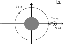
(a)	(b)

Figure 5: The $B=0$ component of the monodromy locus consists of four points on the $a_{0}$-plane containing the base point (cross mark). Among them, only $a_{0-out}$ lies in the 8D gauge theory region $|\epsilon_{K}^{2}\epsilon_{\eta}|\ll|a_{0}|$, and all others $a_{0-4,5,6}\sim{\cal O}(\epsilon_{K}^{2}\epsilon_{\eta})$ are located outside of the 8D gauge theory region (in a shaded region in (a)).

There is only one monodromy locus $a_{0-out}$ in the 8D gauge theory region $|\epsilon_{K}^{2}\epsilon_{\eta}|\ll|a_{0}|$, but three new types of monodromy loci appear in the $a_{0}\sim{\cal O}(\epsilon_{K}^{2}\epsilon_{\eta})$ region. We can think of various loops drawn in Figure 5; it is clearly a question of interest what the monodromy of 2-cycles will be for those loops.

Note that we do not have to consider the $A=0$ component of the monodromy locus any more. In section 3.2, we see that the monodromy of the loop $\gamma_{2-A}$ is trivial. For any loops $\gamma_{A}$ in the moduli space (except $A=0$ and $B=0$) that are homotopic to a loop of the form

$$\gamma_{A}=\gamma_{B}^{-1}\circ\gamma_{2-A}\circ\gamma_{B}$$ (41)

for some loop $\gamma_{B}$, $\rho(\gamma_{A})={\rm id}.$, because $\rho(\gamma_{2-A})={\rm id}.$. Thus, we focus only on the monodromy of the loops which go around the $B=0$ component (38) in the following.

Among the loops in the $a_{0}$ plane in Figure 5, $\gamma_{0-out}$ and $\gamma_{0-\theta}$ stay within the 8D gauge theory region of the moduli space. Direct computation of the monodromy $\rho(\gamma_{0-out})$ shows that

$$\rho(\gamma_{0-out})=W_{C_{A76}}=\rho(\gamma_{2-1}).$$ (42)

This is actually expected, because the loop $\gamma_{0-out}$ is homotopic to $\gamma_{2-1}$ in the $(a_{0},a_{2},a_{3},g_{0})$ moduli space without the $B=0$ monodromy locus. One can also see that $\gamma_{2-2}\sim\gamma_{0-\theta}\circ\gamma_{0-out}\circ\gamma_{0-\theta}^{-1}$ and $\gamma_{2-3}\sim\gamma_{0-\theta}^{-1}\circ\gamma_{0-out}\circ\gamma_{0-\theta}$, and hence the following relations

$$\rho(\gamma_{0-\theta})\rho(\gamma_{0-out})\rho(\gamma_{0-\theta})^{-1} = \rho(\gamma_{2-2})=W_{C_{A76}+C_{-\theta}},$$ (43)

$$\rho(\gamma_{0-\theta})^{-1}\rho(\gamma_{0-out})\rho(\gamma_{0-\theta}) = \rho(\gamma_{2-3})=W_{C_{A76}+C_{-\theta}}$$ (44)

should hold true. We confirmed these relations by explicit computation of the monodromy $\rho(\gamma_{0-\theta})$. Other loops in Figure 5 in the $a_{0}$ plane, which go away from the 8D gauge theory region of the moduli space, are not homotopic at least apparently to the loops whose monodromy we have already calculated.

The full monodromy group of the 2-cycles is a representation of the fundamental group of the $(a_{0},a_{2},a_{3},g_{0})$ moduli space from which the $B=0$ monodromy locus is deleted, and this is what we are interested in. The monodromy group observed in the gauge theory description on 7+1 dimensions, however, correspond to the representation of a subgroup generated only by loops that stay within the 8D gauge theory region of the moduli space. The monodromy group on the 2-cycles split into direct product of the one on ${\rm Span}_{\mathbb{Z}}\{C_{A76},C_{-\theta}\}$ and the one on ${\rm Span}_{\mathbb{Z}}\{C_{\alpha,\beta}^{1,2}\}$ at this level of analysis. The loops such as $\gamma_{0-4,5,6}$ in Figure 5, however, may not be contained in this subgroup, and in general, the full monodromy group is larger than the expectation from the gauge theory description on 7+1 dimensions. Exactly the same thing can be said about the monodromy group of 2-cycles of a family of elliptic K3 manifold parametrized by $(c_{0},c_{1},c_{2},g_{0})$.

3.4 The monodromy beyond the 8D gauge theory region

We first show that the full monodromy group of the family (11) with $(a_{0},a_{2},a_{3},g_{0})$ moduli space is indeed larger than the monodromy group expected from the gauge theory description on 7+1 dimensions. This is done by calculating the monodromy of the loops $\gamma_{0-4,5,6}$ in Figure 5; this is to probe physics and geometry of a region of small $a_{0}$, where the $E_{8}$ gauge theory description on 7+1 dimensions breaks down. We then move on to study the monodromy group of the family for the factorization limit parametrized by $(c_{0},c_{1},c_{2},g_{0})$.

The monodromy for the loops $\gamma_{0,4,5,6}$ can be computed by the same method as in the preceding sections; the calculation for the loop $\gamma_{0-4}$ is demonstrated explicitly in the appendix A. It turns out that the monodromy of $\gamma_{0-4}$ is

$$\tilde{C}_{A65} = C_{A65},\;\;\;\;\;\;\tilde{C}_{A76}=C_{A76}+C_{-\theta}-C_{\alpha}^{1},$$

$$\tilde{C}_{\alpha}^{1} = C_{\alpha}^{1},\;\;\;\;\;\;\tilde{C}_{\alpha}^{2}=C_{\alpha}^{2}+C_{\alpha}^{1}-C_{-\theta},$$

$$\tilde{C}_{\beta}^{1} = C_{\beta}^{1},\;\;\;\;\;\;\tilde{C}_{\beta}^{2}=C_{\beta}^{2},$$ (45)

or equivalently,

$$\rho(\gamma_{0-4})=\left(\begin{array}[]{cc|cc|c}1&&&&\\ 1&-1&&-1&\\ \hline\cr-1&2&1&1&\\ &&&1&\\ \hline\cr&&&&{\bf 1}_{2\times 2}\end{array}\right)$$ (46)

when we choose the basis as $(C_{A76},C_{-\theta},C_{\alpha}^{1},C_{\alpha}^{2},C_{\beta}^{1},C_{\beta}^{2})$. The monodromy matrix $\rho(\gamma_{0-4})$ is trivial on the 2-cycles in the visible $E_{6}$ and hidden $E_{8}$. Similarly, the monodromy for $\gamma_{0-5}$ is given by

$$\tilde{C}_{A65} = C_{A65},\;\;\;\;\;\;\tilde{C}_{A76}=C_{A76}+C_{-\theta}-C_{\alpha}^{1}+C_{\beta}^{1},$$

$$\tilde{C}_{\alpha}^{1} = C_{\alpha}^{1},\;\;\;\;\;\;\tilde{C}_{\alpha}^{2}=C_{\alpha}^{2}+C_{\alpha}^{1}-C_{\beta}^{1}-C_{-\theta},$$

$$\tilde{C}_{\beta}^{1} = C_{\beta}^{1},\;\;\;\;\;\;\tilde{C}_{\beta}^{2}=C_{\beta}^{2}-C_{\alpha}^{1}+C_{\beta}^{1}+C_{-\theta},$$ (47)

and, finally, the one for $\gamma_{0-6}$ is

$$\tilde{C}_{A65} = C_{A65},\;\;\;\;\;\;\tilde{C}_{A76}=C_{A76}+C_{-\theta}-C_{\beta}^{1},$$

$$\tilde{C}_{\alpha}^{1} = C_{\alpha}^{1},\;\;\;\;\;\;\tilde{C}_{\alpha}^{2}=C_{\alpha}^{2},$$

$$\tilde{C}_{\beta}^{1} = C_{\beta}^{1},\;\;\;\;\;\;\tilde{C}_{\beta}^{2}=C_{\beta}^{2}+C_{\beta}^{1}-C_{-\theta}.$$ (48)

The 2-cycles inside the $E_{8}$ root lattice and $C_{\alpha,\beta}^{1,2}$ are mixed up under the monodromy $\rho(\gamma_{0-4,5,6})$. This clearly shows that the loops $\gamma_{0-4,5,6}$ are not homotopic to the loops that stay within the 8D gauge theory region of the moduli space. More importantly, $\rho(\gamma_{0-4,5,6})$ should be added to the list of generators of the full monodromy group; the full monodromy group is no longer the product of the $\mathop{\rm SU}(3)_{\rm str}$ Weyl group $S_{3}$ on the visible $E_{8}$ and something acting on the four 2-cycles $C_{\alpha,\beta}^{1,2}$, but the full monodromy group is larger than that.

The subject of our real interest is the monodromy group of 2-cycles at the factorization limit (24–28). Although we have seen that the monodromy subgroup generated by loops in the constant $(c_{0},c_{1},g_{0})$ slice in the 8D gauge theory region is the $\mathbb{Z}_{2}$ subgroup of the Weyl group $S_{3}$, there may be other generators in the full monodromy group, and the full monodromy group may be larger than $\mathbb{Z}_{2}$. To find out candidates for such a generator, let us take a constant $(c_{1},c_{2},g_{0})$ slice of the moduli space and look at the complex $c_{0}$ plane.

The monodromy locus $B=0$ in (38) should now be rewritten in terms of $c_{0},c_{1},c_{2}$. At the leading order in $\epsilon_{K}$, it becomes

$$B_{{\rm leading}}=(c_{0})^{6}(4c_{0}c_{2}-c_{1}^{2})(c_{0}c_{2}+c_{1}^{2})^{2},$$ (49)

and hence it appears as in Figure 6 (a).

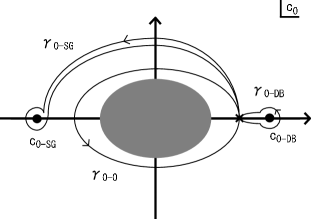
(a)	(b)

Figure 6: The monodromy locus appearing in the constant $(c_{1},c_{2},g_{0})$ slice of the moduli space, and non-trivial loops that go around them. We have chosen a slice that contains the base point (31). The panel (a) is a coarse picture based on $B_{\rm leading}=0$, where higher order corrections in $\epsilon_{K}$ are ignored. The three loops, $\gamma_{0-DB}$, $\gamma_{0-SG}$ and $\gamma_{0-0}$ stay within the 8D gauge theory region, away from the shaded region $|c_{0,*}|\lesssim\epsilon_{K}$. The panel (b) is a fine picture where higher order terms in $\epsilon_{K}$ are not dropped from $B=0$. The $c_{0}=0$ monodromy point with the multiplicity 6 in $B_{\rm leading}=0$ (gray blob in the panel (a)) now splits into 6 distinct points; we can thus find six loops $\gamma_{0-4,5,6}^{1,2}$ in moduli space. The $c_{0-DB}$ monodromy point with multiplicity 2 in the panel (a) also splits into two points $c_{0-DB}^{1,2}$, and two loops $\gamma_{0-DB}^{1,2}$ are found.

However, it was our motivation to study the geometry directly instead of gauge theory descriptions, to take account of higher order corrections in $\epsilon_{K}$, and also to study the region with small $c_{0}$. With all the higher order terms of $B=0$ maintained, Figure 6 (b) is the precise picture of the monodromy locus appearing in the $c_{0}$ plane. It is important to note that the double point $c_{0-DB}$ in Figure 6 (a) splits into two points, $c_{0-DB}^{1,2}$ in Figure 6 (b), due to the higher order terms in $\epsilon_{K}$ in $B=0$. The split in the $c_{0}$ plane is approximately

$$\Delta c_{0-DB}^{1,2}=\pm\frac{\sqrt{3f}}{2}c_{2}\sim\mathcal{O}(\epsilon_{K}^{2}\epsilon_{\eta}^{\frac{1}{2}}),$$ (50)

which shows clearly that this is a higher order effect in $\epsilon_{K}$. The split is certainly small, but still non-zero. Thus, the loops $\gamma^{1,2}_{0-DB}$ that go around either one of them can be separately non-trivial topologically in the moduli space; they may even become extra generators of the monodromy group. Each one of the $a_{0}=a_{0-4,5,6}$ monodromy locus points in the $a_{0}$ plane (Figure 5) splits into a pair $c_{0-4}^{1,2},c_{0-5}^{1,2},c_{0-6}^{1,2}\sim\mathcal{O}(\epsilon_{K}\epsilon_{\eta}^{\frac{1}{2}})$ in the $c_{0}$ plane, because of the factorization condition (26). There are six loops $\gamma_{0-4,5,6}^{1,2}$ that go around them in the $c_{0}$ plane, and they might also generate extra monodromy of the 2-cycles.

We found by numerical study that the motion of 7-branes in the $z$ plane along the loops $\gamma_{0-4,5,6}^{1,2}$ in the $c_{0}$-plane is topologically the same as those along certain combinations of the loops $\gamma_{0-4,5,6}$ in the $a_{0}$-plane. Thus, the monodromy of the loops $\gamma^{1,2}_{0-4,5,6}$ in the $c_{0}$ plane is given by

$$\rho(\gamma_{0-4}^{1}) = \rho(\gamma_{0-4}),\;\;\;\;\;\;\rho(\gamma_{0-4}^{2})=\rho(\gamma_{0-4}),$$

$$\rho(\gamma_{0-5}^{1}) = \rho(\gamma_{0-5}),\;\;\;\;\;\;\rho(\gamma_{0-5}^{2})=\rho(\gamma_{0-4})\rho(\gamma_{0-5})\rho(\gamma_{0-4})^{-1},$$

$$\rho(\gamma_{0-6}^{1}) = \rho(\gamma_{0-6}),\;\;\;\;\;\;\rho(\gamma_{0-6}^{2})=\rho(\gamma_{0-4})^{-1}\rho(\gamma_{0-6})\rho(\gamma_{0-4}).$$ (51)

This clearly shows that the loops digging into the $c_{0}\simeq 0$ region give rise to monodromy of 2-cycles that have not been observed in the gauge theory descriptions on 7+1 dimensions; 2-cycles within the visible $E_{8}$ and those that are not are mixed up under the monodromy (51).

An U(1) symmetry that survives all these monodromies correspond to a six-component row vector that remain invariant after multiplying any one of these monodromy matrices (33, 51) from the right. There is none. We therefore conclude that the U(1) symmetry remaining in the S[U(2)$\times$U(1)] Higgs bundle compactification is broken in the full geometry of F-theory compactification that has a region with $c_{0}=0$ on $S_{GUT}$. The problem B is indeed a problem.

To determine the monodromy associated with the loops $\gamma_{0-DB}^{1,2}$, one only needs to note that the motion of 7-branes in the $z$ plane along these loops are topologically the same as those along the loop $\gamma_{0-out}$ in the $a_{0}$-plane. Thus,

$$\rho(\gamma_{0-DB}^{1,2})=\rho(\gamma_{0-out})=W_{C_{A76}}.$$ (52)

These loops generate monodromy of 2-cycles in the visible $E_{8}$; combining this new generator and the one (33) that we already know in the gauge theory description on 7+1 dimensions, the whole $S_{3}$ Weyl group is generated. We have thought that the monodromy of 2-cycles is reduced from $S_{3}$ to $\mathbb{Z}_{2}$ in the factorization limit of the spectral surface, but because of the $\epsilon_{K}$-suppressed higher order terms that were simply ignored in the 8D gauge theory description, actually the monodromy is not reduced from $S_{3}$. We conclude that there is no unbroken U(1) symmetry with non-trivial components in the visible $E_{8}$ that survives the monodromy generated by both (33) and (52). The problem A is a problem indeed.

To summarize, the full monodromy group contains at least (33), (51) and (52) as generators, maybe more, when the spectral surface is in the factorization limit (26–28). There is no unbroken U(1) symmetry with non-trivial components in the visible $E_{8}$ under the full monodromy group. Thus, we cannot expect an unbroken U(1) symmetry in the low-energy effective theory in ruling out the dimension-4 proton decay operators.

3.5 Non-K3-fibred 4-fold $X_{4}$

We have so far used a Calabi–Yau 4-fold $X_{4}$ that is a K3-fibration on $S_{GUT}$. However, this is just for a concreteness. The monodromy analysis certainly needs to be phrased for individual cases for $X_{4}$’s that are not K3-fibration over $S_{GUT}$. But the essence of the problem A and B, and the essence of analysis remain the same. Let us take simplest non-K3 fibered models as examples: $B_{3}=\mathbb{P}^{3}$, and $S_{GUT}$ is a quadratic ($d=2$) or cubic ($d=3$) surface of $B_{3}$, the models discussed in [12]. First, $A_{k}$ in (2) are set to be [28]

$$A_{k}=s^{k-1}\tilde{A}_{k},\qquad\tilde{A}_{k}\in\Gamma(B_{3};{\cal O}_{B_{3}}(-kK_{B_{3}}-(k-1)S_{GUT})),$$ (57)

where $s$ is a global holomorphic section of ${\cal O}_{B_{3}}(S_{GUT})\simeq{\cal O}_{\mathbb{P}^{3}}(dH)$ whose zero locus is the GUT divisor $S_{GUT}$. $a_{6-k}$ on $S_{GUT}$ in (3) correspond to $\tilde{A}_{k}|_{S_{GUT}}$. Suppose that a point $p_{0}\equiv[0:0:0:1]\in\mathbb{P}^{3}$ is not contained in $S_{GUT}$. The base manifold except this point, $\mathbb{P}^{3}\backslash p_{0}$ is covered by three patches $\simeq\mathbb{C}^{3}$, which constitute ${\cal O}_{\mathbb{P}^{2}}(1)$. Restriction of the original elliptic fibration over $B_{3}=\mathbb{P}^{3}$ to that over ${\cal O}_{\mathbb{P}^{2}}(1)$, combined with a projection $\pi_{0}:{\cal O}_{\mathbb{P}^{2}}(1)\rightarrow\mathbb{P}^{2}$ defines a complex surface fibration

$$\pi_{0}\circ\pi_{X}:\pi^{-1}_{X}\left({\cal O}_{\mathbb{P}^{2}}(1)\right)\rightarrow\mathbb{P}^{2}.$$ (58)

The fiber of this map is an elliptic fibration over $\mathbb{C}$, with 48 discriminant points on the $\mathbb{C}$ plane. Although the number of $[p,q]$ 7-branes is not the same as in the case of an elliptic K3 manifold, independent topological 2-cycles and their intersection form of the fiber complex surface can be worked out by using the techniques in [29, 17]. Monodromy can be studied for loops in $\mathbb{P}^{2}$. When $d\neq 1$, other points $p_{i}$’s in $B_{3}=\mathbb{P}^{3}$ should also be chosen so that the analysis for $\pi_{i}:\mathbb{P}^{3}\backslash p_{i}\simeq{\cal O}_{\mathbb{P}^{2}}(1)\rightarrow\mathbb{P}^{2}$ is carried out and all the ramification locus of the projection $\pi_{i}|_{S_{GUT}}:S_{GUT}\rightarrow\mathbb{P}^{2}$ is covered by some of the analysis of $\mathbb{P}^{3}\backslash p_{i}$. Generalization from these examples to, e.g., toric $B_{3}$ (c.f. [30]), is straightforward.

The problem A arises from the difference between $a_{6-k}=\tilde{A}_{k}|_{S_{GUT}}$ and $\tilde{A}_{k}$, and the problem B arises essentially because of the local behavior of 2-cycles wherever $a_{0}$ vanishes. Thus, we expect similar phenomena also in the case of $B_{3}=\mathbb{P}^{3}$, though we have not done the analysis. Since more than one points of $S_{GUT}$ are projected onto the same point in $\mathbb{P}^{2}$ for $d\neq 1$, 2-cycles in $E_{8}$ on a point of $S_{GUT}$ may mix with 2-cycles in $E_{8}$ on another point of $S_{GUT}$ in the context of problem B.

4 Consequences in Physics

4.1 U(1) Violating State-Mixing and Trilinear Couplings

We have studied a model of $E_{8}\rightarrow E_{6}$ symmetry breaking with a spectral surface in the 2+1 factorization limit in the previous section, as a toy model of $E_{8}\rightarrow{\rm SU}(5)_{\rm GUT}$ symmetry breaking in a certain factorization limit. On the contrary to the expectation in gauge theory in 7+1 dimensions, the study shows that there is no monodromy-invariant 2-cycle, and hence there is no unbroken U(1) symmetry in the low-energy effective theory below the Kaluza–Klein scale. Without an unbroken U(1) symmetry, we generally expect that dimension-4 proton decay operators will be generated. In this section, we discuss whether the dimension-4 proton decay operators are really generated from known interactions in string theory.

In F-theory, charged matter fields come from the degree of freedom of M2-branes wrapping on the 2-cycles corresponding to the representation of charged matters. Trilinear interactions are (likely to be) generated, if the sum of 2-cycles for the three fields is topologically trivial. Thus, by using this criterion, we can check whether dimension-4 proton decay operators are generated or not.

In the $E_{8}\rightarrow E_{6}$ symmetry breaking model with the 2+1 factorization, the matter curve for $E_{6}$-27 representation splits into two irreducible pieces; one is characterized by $c_{2}=0$, and the other by $d_{1}=-c_{1}=0$. Based on the gauge theory description on $S_{GUT}$, one would expect that the charged matter fields in the $E_{6}\times{\rm U}(1)$-${\bf 27}_{+1}$ representation are localized along the $c_{2}=0$ curve in $S_{GUT}$, and those in the ${\bf 27}_{-2}$ along the $c_{1}=0$ curve. Ignoring the monodromy that we studied in section 3.4, the 2-cycle $(C_{A76}+C_{A65})$ vanishes along the $c_{1}=0$ curve, while either $C_{A65}$ or $(C_{-\theta}+C_{A76}+C_{A65})$ does along $c_{2}=0$. $4c_{0}c_{2}-c_{1}^{2}=0$ is the ramification locus of the 2-fold spectral cover, where monodromy $W_{C_{A76}+C_{-\theta}}$ exchanges $C_{A65}$ and $(C_{-\theta}+C_{A76}+C_{A65})$. See Figure 7.

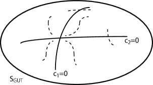
Figure 7: A schematic picture of matter curves and monodromy loci on $S_{GUT}$. The ramification locus $c_{1}^{2}-4c_{2}c_{0}\simeq 0$ and a locus $(2c_{1}^{2}+c_{2}c_{0})\simeq 0$ with multiplicity 2 both approach the points of enhanced $E_{8}$ singularity. The multiplicity-2 branch, however, has a small split, and consists of two branches with multiplicity 1. Furthermore, all the three branches form a single irreducible component monodromy locus $B=0$ around $(c_{1},c_{2})\simeq(0,0)$. The monodromy locus $B=0$ also intersect the matter curves at $(c_{1},c_{0})\simeq(0,0)$ and $(c_{2},c_{0})\simeq(0,0)$.

The trilinear interaction $\Delta W={\bf 27}_{+1}\cdot{\bf 27}_{+1}\cdot{\bf 27}_{-2}$ is generated at $E_{8}$ singularity enhancement points $c_{1}=c_{2}=0$, because all the three 2-cycles vanish simultaneously there, and they satisfy

$$(C_{-\theta}+C_{A76}+C_{A65})+C_{A65}+(C_{A76}+C_{A65})\equiv 0\quad({\rm mod~{}}E_{6}).$$ (59)

This Yukawa coupling is invariant under the U(1) symmetry.

We know, however, that there are more monodromy among the 2-cycles. Under the monodromy (52), the 2-cycle $C_{A65}$ for ${\bf 27}_{+1}$ turns into $(C_{A76}+C_{A65})$ for ${\bf 27}_{-2}$ and vice versa. The matter fields in the $E_{6}$-${\bf 27}$ representation cannot remain pure eigenstates of the U(1) symmetry. This mixing among states with different U(1) charges (and hence the monodromy) takes place around the monodromy locus

$$(c_{0,*})^{4}(c_{0,*}c_{2,*}+2c_{1,*}^{2})^{2}\simeq 12f_{0}(\epsilon_{K})^{4}(c_{1,*}^{2})^{4},$$ (60)

which is a part of $B=0$ locus, just like the ramification locus $4c_{0}c_{2}-c_{1}^{2}\simeq 0$. Since this branch also approach the $c_{1}=c_{2}=0$ point just like the ramification locus (see Figure 7), we do not have a reason to believe that the mixing (monodromy) due to this branch cancels, while that of the ramification locus remain. The mixing may be suppressed by some function of $\epsilon_{K}$, but we cannot take $\epsilon_{K}$ to be literally zero in (5, 6, 15, 29) in $\mathop{\rm SU}(5)_{\rm GUT}$ models. Therefore, all sorts of U(1) violating trilinear interactions $\Delta W={\bf 27}\cdot{\bf 27}\cdot{\bf 27}$ will be generated, unless there is a cancellation.

There are other groups of regions in $S_{GUT}$ where the matter curves $c_{1}=0$ or $c_{2}=0$ encounters the $B=0$ monodromy locus. One is $c_{0}\simeq 0$ on $c_{1}\simeq 0$ ($c_{2,*}\neq 0$), and the other is $c_{0}\simeq 0$ along $c_{2}\simeq 0$ ($c_{1,*}\neq 0$). The monodromy we studied in section 3.4 is relevant to the latter. The 2-cycle $(C_{-\theta}+C_{A76}+C_{A65})$ for ${\bf 27}_{+1}$ and $(C_{A76}+C_{A65})$ for ${\bf 27}_{-2}$ are exchanged under the monodromy (51) modulo 2-cycles $C_{\alpha,\beta}^{1,2}$. Thus, the “${\bf 27}_{+1}$” fields will have non-vanishing $[C_{A76}+C_{A65}]$ (mod $C_{\alpha,\beta}^{1,2}$) component and vice versa. The mixing, however, will presumably be suppressed exponentially, because it is 2-cycles of finite size, rather than vanishing 2-cycles, that are exchanged under the monodromy at $c_{0}\simeq 0$.

The U(1) symmetry violating Yukawa couplings ${\bf 27}\cdot{\bf 27}\cdot{\bf 27}$ are generated only when the sum of three topological 2-cycles vanish in $H_{2}({\rm K3};\mathbb{Z})$, just like in (59). Thus, just a single monodromy out of (51) acting on $(C_{-\theta}+C_{A76}+C_{A65})$ does not generate such a U(1) violating coupling ${\bf 27}$;

$$(C_{-\theta}+C_{A76}+C_{A65})+C_{A65}+(\tilde{C}_{-\theta}+\tilde{C}_{A76}+\tilde{C}_{A65})\neq 0$$ (61)

in $H_{2}({\rm K3};\mathbb{Z})$ (mod $E_{6}$). After exploiting all the monodromies available in a 4-fold $X_{4}$ that is a K3 fibration on $S_{GUT}$, however, all $C_{\alpha,\beta}^{1,2}$ will be mixed up and twisted over $S_{GUT}$, and eventually such a U(1) violating coupling will be generated, although the coupling constant may be highly suppressed. In the case of non-K3 fibred $X_{4}$, $H_{2}({\rm K3};\mathbb{Z})$ just has to be replaced by $H_{2}$ of the complex-surface fibration of (58).

The renormalizable proton decay operators are not the only consequence of the U(1) symmetry-breaking state mixing. Factorized spectral surface limit has been used for dimension-5 proton decay problem [11], or for the purpose of exploiting [31, 32] the idea of flavor structure in [33, 7, 8, 34]. The discussion so far implies that it is impossible to confine $\bar{\bf 5}_{H}$ and ${\bf 5}_{H}$ to separate irreducible pieces of $\mathop{\rm SU}(5)_{\rm GUT}$ matter curves completely. This may not be a big problem, as opposed to the dimension-4 proton decay problem, however, because the dimension-5 proton decay problem only requires a small amount of suppression; complete separation is not necessary. In the context of flavor structure of Yukawa couplings, the three copies of the visible sector matter fields $\bar{\bf 5}_{M}$ or ${\bf 10}_{M}$ may not be able to have wavefunctions strictly in a single irreducible component of the factorized matter curves, even at the factorization limit of the spectral surface. This means that the up-type Yukawa matrix of the low-energy effective theory below the Kaluza–Klein scale receives contributions from more than one point of enhanced $E_{6}$ singularity [31, 32]. If the state mixing is small, then this mixing is not terribly bad, and may even contribute in generating smaller eigenvalues; the flavor structure generated in this way is not necessarily similar to the one we observe in the Standard Model, however.

It should be remembered, however, that our analysis employed a 2+1 factorization in the $E_{8}\rightarrow E_{6}$ symmetry breaking. Thus, it will not be a terribly bad guess to expect similar results for the 4+1 and 3+2 factorization in the $E_{8}\rightarrow\mathop{\rm SU}(5)_{\rm GUT}$ symmetry breaking [10, 6, 11]. When another type of factorization (or monodromy subgroup of $S_{5}$) is employed, as in [14, 15], separate study is necessary, especially because it is not clear how the problem A will look like in such a factorization limit.

4.2 Loopholes in This Argument

The discussion so far hints that the dimension-4 proton decay operators are generated in the factorized spectral surface scenario. There are some loopholes in the argument, however. At the end of this article, here, we list up some loopholes that come to our minds. The list can also be taken as possible ways to save the factorized spectral surface solution.

First of all, the argument so far only showed that

• there is no unbroken U(1) symmetry (apart from exceptional cases that we discuss later) in the low-energy effective theory that we hope would exclude the dimension-4 proton decay operators, and

• the picture of interactions as recombination of M2-branes without a change in the total topology does not exclude the U(1) violating operators.

It is not that we have calculated the coefficients of such operators, and in fact, we do not even have a theoretical framework to calculate the coefficients within F-theory. A gauge theory on 7+1 dimensions cannot handle this. A possible direction is to exploit the Type IIB–M-theory duality or F-theory–Heterotic duality; dual descriptions may be used to see whether cancellation mechanism is likely to exist, or to make an estimate of the coefficients. That will tell us how small $\epsilon_{K}$ should be. Such a study is beyond the scope of this article, however.

If one literally sets $\epsilon_{K}=0$, instead of fine-tuning it to be sufficiently small, then $S_{GUT}$ becomes a locus of $E_{8}$ singularity. If a vector bundle on $S_{GUT}$ has a structure group that is smaller than $\mathop{\rm SU}(5)_{\rm str}\times\mathop{\rm U}(1)_{Y}$ so that an extra U(1) factor is contained, then an unbroken U(1) symmetry remains in the low-energy effective theory and prevent proton decay. The chirality of various charged matter fields in this case, however, are determined simply by intersection numbers of first Chern classes of those bundles and $K_{S_{GUT}}$ [10, 2, 3, 24], and existence of exotics is predicted easily [10, 12, 11]. It is also obvious that theories of flavor structure like those in [4, 33, 35, 7, 31, 32] are not applied to such a case, because only $A_{4}$ singularity is assumed along $S_{GUT}$.

Secondly, one will notice that our analysis in section 3 is based on a choice (26–28) of the solution to (25). The condition (25), however, can be solved in the form of

$$c_{0}=ps,\quad d_{1}=-qr,\quad c_{1}=pr,\quad d_{0}=qs$$ (62)

for some global holomorphic sections

$$s\in\Gamma(S_{GUT};{\cal O}_{S}(\eta_{0})),\quad p\in\Gamma(S_{GUT};{\cal O}_{S}(\eta^{\prime}_{1})),\quad q\in\Gamma(S_{GUT};{\cal O}_{S}(\eta^{\prime}_{2})),$$ (63)

$$r\in\Gamma(S_{GUT};{\cal O}_{S}(\eta_{0}+K_{S_{GUT}}));$$ (64)

here, $\eta^{\prime}_{1,2}$ and $\eta_{0}$ are some divisors on $S_{GUT}$, and $c_{2}\in\Gamma(S_{GUT};{\cal O}_{S}(\eta^{\prime}_{1}+\eta_{0}+2K_{S_{GUT}}))$. What we studied in section 3 is the monodromy associated with $s=0$ locus.

What if the global section $s$ does not have a zero locus? This is possible if the line bundle ${\cal O}_{S}(\eta_{0})$ is trivial; $s$ can now take a constant non-zero value over the entire $S_{GUT}$. Suppose that this topological condition is satisfied. If we further assume that the divisor $K_{S_{GUT}}$ is not effective, as in del Pezzo surfaces and Hirzebruch surfaces, then there is no non-trivial global holomorphic section $r$. We have to set $r=0$. This means that

$$c_{1}=d_{1}=0$$ (65)

over the entire $S_{GUT}$, which is nothing but the case we already listed as the rank-5 GUT scenario (ii) in Introduction. The dimension-4 proton decay problem can be solved completely in this scenario, because of an unbroken (or spontaneously broken) U(1) symmetry in the low-energy effective theory; an extra 2-cycle is along $S_{GUT}$, and a semi-local geometry of this form along $S_{GUT}$ is sufficient in ensuring the proton stability [10]. The singularity along $S_{GUT}$ is either $D_{5}$ or $A_{5}$ in this case, and theories of flavor structure [4, 33, 35, 7, 31] are not applied here. Exotic-matter free conditions have also been studied for rank-5 GUT scenarios [12, 36].

If the divisor $K_{S_{GUT}}$ is effective, on the other hand, we can introduce a different set of topological conditions: all of line bundles ${\cal O}_{S}(\eta_{0})$ and ${\cal O}_{S}(\eta^{\prime}_{1,2})$ are trivial, so that there is no zero locus in $s$, $p$ and $q$. This is possible for an effective $K_{S_{GUT}}$, because the matter curves belong to topological classes of effective divisors. Now there is no $a_{0}=0$ locus, and at least the problem B is gone, under this set of topological conditions.

An obvious loophole in the argument that follows (7) is that the coefficient of the highest degree term $a_{5-k}$ may not have a zero locus. We have already exploited a case that $a_{0}$ is constant and non-zero, and a remaining alternative is a case where $a_{2}$ is constant and non-zero everywhere on $S_{GUT}$. This is possible only when $K_{S_{GUT}}$ is effective on $S_{GUT}$, and $a_{0}\in\Gamma(S_{GUT};{\cal O}_{S}(-2K_{S_{GUT}}))$ vanishes as a consequence. An $E_{7}$ gauge theory is well-defined over the entire $S_{GUT}\times\mathbb{R}^{3,1}$. There is no mixing between 2-cycles in $E_{7}$ and those outside, and the problem B is gone in this case. What is more intriguing in this model is that there is no need to impose a factorization condition like (24) by hand. The commutant of $\mathop{\rm SU}(5)_{\rm GUT}$ in $E_{7}$ is $\mathop{\rm U}(3)$. The decomposition

$${\rm Res}^{E_{7}}_{\mathop{\rm U}(3)\times\mathop{\rm SU}(5)_{\rm GUT}}{\bf adj.} = ({\bf adj.},{\bf 1})+({\bf 1},{\bf adj.})$$ (66)

$$+ \left[({\bf 3},\overline{\bf 10})+(\wedge^{2}{\bf 3},{\bf 5})+(\wedge^{3}{\bf 3},\bar{\bf 5})\right]+{\rm h.c.}$$

shows that there are two different kinds of charged matter fields in the $\mathop{\rm SU}(5)_{\rm GUT}$-$\bar{\bf 5}$ representation. For a fully generic 3-fold spectral cover globally defined on $S_{GUT}$, $({\bf 3},\overline{\bf 10})+(\bar{\bf 3},{\bf 10})$ matter fields are localized along the $a_{5}=0$ locus, while $(\wedge^{2}{\bf 3},{\bf 5})+{\rm h.c.}$ and $(\wedge^{3}{\bf 3},\bar{\bf 5})+{\rm h.c.}$ matter fields are localized along the $(-a_{2}a_{5}+a_{4}a_{3})=0$ and $a_{3}=0$ loci, respectively. This factorization / decomposition automatically takes place under this topological condition. Because of the commutation relation of the $E_{7}$ Lie algebra, $(\wedge^{2}{\bf 3},{\bf 5})$ is identified with the origin of the up-type Higgs multiplet. If $(\wedge^{3}{\bf 3},\bar{\bf 5})$ and $(\wedge^{2}\bar{\bf 3},\bar{\bf 5})$ are identified with $\bar{\bf 5}_{H}$ and $\bar{\bf 5}_{M}$, respectively, then the moduli $({\bf adj.},{\bf 1})$ for the $\mathop{\rm U}(3)$ spectral surface may become right-handed neutrinos [14, 6]. The up-type Yukawa couplings and down-type/charged lepton Yukawa couplings originate from

$$\Delta W=\left(\wedge^{4}{\bf 8}\right)^{MNPQ}\cdot{\bf adj.}^{I}_{\;H}\cdot\left(\wedge^{4}{\bf 8}\right)^{HJKL}\;\epsilon_{IJKLMNPQ}$$ (67)

in the language of $\mathfrak{su}(8)\subset\mathfrak{e}_{7}$, and the neutrino Yukawa couplings from [10]

$$\Delta W=\mathop{\rm tr}{}_{\mathfrak{su}(8)}\left({\bf adj.},[{\bf adj.},{\bf adj.}]\right).$$ (68)

It is worthwhile to study the monodromy for this case, e.g, using the example in footnote 17, to see how the problem A will look like, because the “problem A” may be quite different in nature, or may even be absent, in such a case without a need for imposing factorization condition by hand.

Finally, there are also loopholes that resort to continuous fine-tuning of complex structure parameters. Flux compactifications should ultimately explain such a tuning. At the level of gauge theory description on 7+1 dimensions, we introduced a parametrization of the complex structure moduli $a_{0}$, $a_{2}$ and $a_{3}$ by $c_{0,1,2}$ as in (26–28), so that the spectral surface factorizes in the new parametrization. But the ultimate goal is to reduce the monodromy of 2-cycles so that an unbroken U(1) symmetry is maintained in the low-energy effective theory. Thus, the generalized version of the solution is to consider a parametrization of the complex structure moduli $(a_{0,2,3},f_{0},g_{0},a^{\prime\prime}_{0})$ of $X_{4}$ so that the polynomial $B$ in (38) is factorized appropriately in the new parameters. The geometry for compactification should be given by holomorphic sections from $S_{GUT}$ to the new parameter space. It will be straightforward to work out the expression for “$B$” in the case of $E_{8}\rightarrow{\rm SU}(5)_{\rm GUT}$ symmetry breaking.

In the case of $E_{8}\rightarrow E_{6}$ symmetry breaking, the polynomial $B$ should be factorized so that the split between $c^{1}_{2-DB}$–$c^{1}_{0-DB}$ and $c^{2}_{2-DB}$–$c^{2}_{0-DB}$ disappears and they form a monodromy locus of multiplicity 2. The monodromy (52) is gone in this limit; this is a fine-tuning solution to the problem A.

A hint for a fine-tuning solution to the problem B comes from Heterotic dual description. In Heterotic string language, one can tune complex structure moduli so that the elliptic fibred Calabi–Yau 3-fold admits a non-trivial section; moduli of spectral surfaces of $V_{1}$ and $V_{2}$ may be tuned so that the line bundle ${\rm det}\;V_{1}$ corresponds to the non-trivial section. In other words, this is to consider the factorization limit of (117) instead of the factorization limit of (8, 10). There still remains a problem of determining the $\epsilon_{\eta}$ suppressed corrections, because the spectral surface picture relies on supergravity + $E_{8}\times E_{8}$ super Yang–Mills approximation in the Heterotic description (see the appendix B for more). In F-theory language, this tuning, we expect, will correspond to factorization of $B$ so that all the six branches $c^{1,2}_{0-4,5,6}$ somehow come on top of one another in the new parametrization space to form a monodromy locus of multiplicity 6. The monodromy, then, is $\rho(\gamma_{0-0})$, which we know is trivial on the $E_{8}$ part of the 2-cycle. We do not have a concrete picture of how to modify the parametrization (26–28) systematically to obtain the new parametrization, however.

Appendix A Some examples of computing the monodromy of 2-cycles

In sections 3.2–3.4, we need to study monodromy of 2-cycles of an elliptic fibered K3 manifold for loops in the moduli space of the elliptic K3; this monodromy group is used in this article, to find out whether an unbroken U(1) symmetry remains in the effective theory and the dimension-4 proton decay operators (1) are ruled out. In order to calculate the monodromy of 2-cycles, we first need to identify 2-cycles in an elliptically fibered K3 surface that constitute a basis of $H_{2}({\rm K3};\mathbb{Z})$. Second, we analyze the changes of the 2-cycles when we move along a loop in the moduli space.

We are not interested so much in the fiber class and base class of the elliptic fibration, because they do not correspond to a U(1) vector field or a U(1) symmetry. When an M2-brane is wrapped on one of other topological 2-cycles of an elliptic K3 manifold, it is interpreted as a string junction configuration on the base manifold $\mathbb{P}^{1}$. The first task, therefore, is to identify “independent” string junction configurations, which has already been done completely in [17]. In section A.1, we briefly review the results of [17], while explaining details of our conventions that are used in the calculation in section A.2.

String junction configurations on $\mathbb{P}^{1}$ are easier to deal with (for string theorist) than topological 2-cycles in an elliptic K3 manifold. Thus, we calculate monodromy of topological 2-cycles by following the configuration of string junctions along a loop in the moduli space of the elliptic K3. We demonstrate the technique of the computation of the monodromy explicitly for some loops as examples in section A.2.

The appendix A constitutes nearly a third of this article, but it is a technical note in nature. The main text will be readable without reading the details of this appendix.

A.1 Independent 2-cycles in the language of string junctions

Let us consider a 7-brane configuration in a complex $z$ plane, where $[1,0]$ 7-branes (called A-branes), $[1,-1]$ 7-brane (called B-branes), $[1,1]$ (C-branes) and $[3,-1]$ 7-branes (we call them “$D$”-branes) are line up from left to right as

$$A^{8}BC^{2}D\;A^{8}BC^{2}D,$$ (69)

and branch cuts run from all of those 7-branes to the infinity in the $z$-plane in the positive imaginary direction. This is the $\hat{E}_{9}\hat{E}_{9}$ configuration in [17], which contains two sets of 7-brane configuration $[A^{7}BC^{2}]$ for $E_{8}$. We assign names to these 7-branes. The eight A-branes on the left are called $A8$–$A1$ from left to right, and the two C-branes on the left called $C1$ and $C2$ from left to right (see Figure 1). The B-brane and “D”-brane on the left are simply called $B$ and $D$. The twelve 7-branes on the right are named similarly, with an extra ^′, such as $A8^{\prime}$, $A7^{\prime}$ etc. We will see shortly that the configuration of $[p,q]$ 7-branes and branch cuts can be made topologically the same as this for an explicit choice of a base point in the elliptic K3 moduli space.

We have adopted a convention that a $(p,q)$ string corresponds to an M2-brane wrapped on $(p\alpha+q\beta)$ cycle of the $T^{2}$-fiber. The $(r,s)$ charge of a string undergoes the monodromy as in

$$\left(\begin{array}[]{c}r\\ s\end{array}\right)\rightarrow M_{p,q}\left(\begin{array}[]{c}r\\ s\end{array}\right)\equiv\left(\begin{array}[]{cc}1-pq&p^{2}\\ -q^{2}&1+pq\end{array}\right)\left(\begin{array}[]{c}r\\ s\end{array}\right)$$ (92)

when the string crosses a branch cut for a $[p,q]$ 7-brane in anti-clockwise direction.

Any string junctions on $\mathbb{P}^{1}$ correspond to closed 2-cycles of an elliptic K3. We can pull out any junction configurations to the negative imaginary direction by continuous deformation, so that the configuration does not cross a branch cut; string creation process should be used if necessary. By deforming junction configurations in this way, we can express junction configurations by 24 integers $N^{i}$, where $i=A8,A7,\cdots,A1,B,\cdots,C1^{\prime},C2^{\prime},D^{\prime}$ run over the twenty four 7-branes; $N^{i}$ are the numbers of $(p_{i},q_{i})$ strings coming out of the $i$-th 7-brane whose charge is $[p_{i},q_{i}]$. For example, the junction configuration (and the 2-cycle) named $C_{A76}$ is characterized by $N^{A7}=1$, $N^{A6}=-1$, and $N^{i}=0$ for all other 7-branes. $C_{BCD}$ corresponds to $N^{B}=N^{C1}=N^{C2}=1$, $N^{D}=-1$, and $N^{i}=0$ for all the other 7-branes. See Figure 1. We denote 22 independent closed 2-cycles by [17]

• visible $E_{8}$: $C_{A76}\sim C_{A21},C_{ABC}$ and $C_{C12}$ (see Figure 1),

• hidden $E_{8}$: $C^{\prime}_{A76}\sim C^{\prime}_{A21},C^{\prime}_{ABC}$ and $C^{\prime}_{C12}$ that are the same string junction configuration as the corresponding ones in visible $E_{8}$, except that their endpoints are on the 7-branes $A8^{\prime}$–$A1^{\prime}$, $B^{\prime}$, $C1^{\prime}$, $C2^{\prime}$ and $D^{\prime}$,

• others: $C_{A87}$, $C_{BCD}$, $C^{\prime}_{A87}$, $C^{\prime}_{BCD}$, $C_{AA^{\prime}}$ and $C_{DD^{\prime}}$ (see Figure 1).

Among the 22 closed 2-cycles listed above, however, 2 linear combinations

$$C_{BCD}+C^{\prime}_{BCD}\quad{\rm and}\quad-C_{A87}+-C_{A87}^{\prime}+C_{-\theta}+C_{-\theta}^{\prime}$$ (93)

can expressed as a boundary of 3-dimensional cells; here, $C_{-\theta}$ is defined by (12), and $C^{\prime}_{-\theta}$ is its obvious ^′ version. We thus drop $C^{\prime}_{BCD}$ and $C^{\prime}_{-\theta}-C^{\prime}_{A87}$, and use $C_{BCD}$, $C_{-\theta}$, $C_{AA^{\prime}}$, $C_{DD^{\prime}}$ and the 16 2-cycles of the visible and hidden $E_{8}$’s as representatives of the 20 independent topological 2-cycles in $H_{2}({\rm K3};\mathbb{Z})$ [17].

For an appropriate choice of a basis of $H_{2}({\rm K3};\mathbb{Z})$, the intersection form becomes [41]

$$-C(E_{8})\oplus\left(\begin{array}[]{cc}0&1\\ 1&0\end{array}\right)\oplus\left(\begin{array}[]{cc}0&1\\ 1&0\end{array}\right)\oplus-C(E_{8}^{\prime}),$$ (98)

where $C(E_{8})$ and $C(E_{8}^{\prime})$ denotes the Cartan matrix of $E_{8}^{(\prime)}$ respectively, with an extra 2 by 2 block for the fiber and base classes. The eight 2-cycles of the visible $E_{8}$ and those of the hidden $E_{8}$ can be used as the first and last eight elements of the basis. The remaining four elements of a basis for the intersection form above can be chosen as the following four linear combinations [17]:

$$C_{\alpha}^{1}=-C_{A87}+C_{-\theta}, C_{\alpha}^{2}=-C_{A87}+C_{-\theta}+C_{AA^{\prime}},$$ (99)

$$C_{\beta}^{1}=C_{BCD}, C_{\beta}^{2}=C_{BCD}+C_{DD^{\prime}}.$$ (100)

$\left\langle{C_{\alpha}^{1},C_{\alpha}^{2}}\right\rangle=1$, $\left\langle{C_{\beta}^{1},C_{\beta}^{2}}\right\rangle=1$, and all other intersection numbers among the four 2-cycles vanish.

A.2 Some examples of the monodromy

A.2.1 The 7-brane configuration at the base point

In section A.2, we present the practical procedure of calculation of monodromy of 2-cycles for some loops in the moduli space of elliptic K3 manifold (11). We have chosen a base point as in (19) in the moduli space.

Figure 8: The 7-brane configuration at the base point (19). The dotted curves represent branch cuts. The approximate location of $A6$ 7-brane is $z_{A6}\sim-\frac{27}{64}\frac{a_{3}^{4}}{a_{2}^{3}}\sim\mathcal{O}(\epsilon_{K}^{6}\epsilon_{\eta}^{1}\delta^{4})$ and $z_{A7}\sim-\frac{4}{27}\frac{a_{2}^{3}}{a_{0}^{2}}\sim\mathcal{O}(\epsilon_{K}^{6}\epsilon_{\eta})$ for $A7$ 7-brane [see also (34)]. $A8$ and $D$ 7-branes are at $z\sim\mathcal{O}(\epsilon_{\eta})$.

The 7-branes configuration on the base $\mathbb{P}^{1}$ at this base point is shown in Figure 8. Since we introduced a small parameter $\delta$ in the definition of the base point, the elliptic K3 manifold for the base point must realize a hierarchical symmetry breaking $E_{8}\rightarrow E_{7}\rightarrow E_{6}$. We thus assign the name A6 to the 7-brane that is closest to the $E_{6}$ point. The branch cuts and the $[p,q]$ charges of the 7-branes are given as in Figure 8. This arrangement is certainly the way anticipated in (69), but it is not trivial whether the cut configuration and charge assignment in the figure are correct for the specific choice of the complex structure at the base point. We confirmed that this is a right choice, by examining the 1-cycles of the $T^{2}$ fiber to degenerate and monodromy of the complex structure of the fiber at these 7-branes.

A.2.2 The Monodromy of the loop $\gamma_{2-A}$

First, we consider the monodromy around the loop $\gamma_{2-A}$. This loop goes around a triple point of the monodromy locus. The loop $\gamma_{2-A}$ is depicted in the Figure 3. We decompose the loop $\gamma_{2-A}$ into three paths in calculating the monodromy.

1. approaching $a_{2}=a_{2-A}$ from the base point from the right (path 1),

2. going around $a_{2}=a_{2-A}$ in the anti-clockwise direction (path 2), and finally,

3. going back to the base point from $a_{2}=a_{2-A}$ (path 3).

The 2-cycles at the base point change when evaluated after they go along path 1, path 2 and path 3. We can read the monodromy matrix from the change of the 2-cycles.

Path 1: The movement of 7-branes corresponding to the path 1 is shown in the first part of the Table LABEL:tb:2-A_path1. After completing the path 1, we rearrange the branch cuts as a preparation for the path 2, by two steps as in the second and third part of the Table LABEL:tb:2-A_path1. The changes of 2-cycles (string junction) as well as the change in the $[p,q]$ charges of various 7-branes during the rearrangement of the branch cuts are also shown in the table below the corresponding figures (Table LABEL:tb:2-A_path1). As we already explained in section A.1, string junction configurations are always deformed continuously so that they do not cross any one of branch cuts. The numbers in the table show the number of $[p_{i},q_{i}]$ strings coming out of a $[p_{i},q_{i}]$ 7-brane.

Table 2: The first figure shows the motion of 7-branes along the path 1. The location of 7-branes before the movement is depicted by the gray circles. The next two figures show how to rearrange branch cuts. The changes of 2-cycles (string junctions) of the process are shown below the corresponding figures. We denotes the $[p,q]$ charge next to the name of 7-branes.

A8 [1,0] A7 [1,0] A6 [1,0] A5 [1,0] A4-A1 [1,0] B [1,-1] C1,2 [1,1] D[3,1] $C_{A76}$ 0 1 -1 0 0 0 0 0 $C_{A65}$ 0 0 1 -1 0 0 0 0 $C_{BCD}$ 0 0 0 0 0 1 1 -1

$\downarrow$ step 1

Passing $A6+E_{6}$ 7-branes through

the branch cuts of $A7$ 7-branes from right to left.

A8 [1,0] A6 [1,0] A5 [1,0] A4-A1 [1,0] B [0,-1] C1,2 [2,1] A7 [1,0] D[3,1] $C_{A76}$ 0 -1 0 0 0 0 1 0 $C_{A65}$ 0 1 -1 0 0 0 0 0 $C_{BCD}$ 0 0 0 0 1 1 -1 -1

$\downarrow$ step 2

Passing $A6$ 7-branes through

the branch cuts of $E_{6}$ 7-branes from left to right.

A8 [1,0] A5 [1,0] A4-A1 [1,0] B [0,-1] C1,2 [2,1] A6 [-3, -1] A7 [1,0] D[3,1] $C_{A76}$ 0 0 0 -1 -1 -1 1 0 $C_{A65}$ 0 -1 0 1 1 1 0 0 $C_{BCD}$ 0 0 0 1 1 0 -1 -1

Path 2: During the path 2, the $A6$ 7-brane and $A7$ 7-brane mutually rotate around the other by $3\pi$, as in Table LABEL:tb:2-A_path2. We have rearranged the branch cuts at the end of path 1, so that they do not cross any branch cuts except the cuts of themselves. Note, however, that $A6$ and $A7$ 7-branes are not mutually local after the rearrangement of the branch cuts. Therefore we have to take a close look during the path 2 at the changes of $[p,q]$ charges of the $A6$ and $A7$ 7-branes, and at the changes of string junction configurations that have end points on $A6$ or $A7$. For every $\pi$ rotation, either $A6$ or $A7$ has to cross the branch cut of the other. Thus, we need to trace the changes of junction configurations for every $\pi$ rotation. Table LABEL:tb:2-A_path2 shows the results. From the Table LABEL:tb:2-A_path2, the 2-cycles do not change after the $3\pi$ rotation.

Table 3: The motion of 7-branes and the changes of the 2-cycles along the path 2. $\tilde{C}$s represent the 2-cycles after $3\pi$ rotation.

A8 [1,0] A5 [1,0] A4-A1 [1,0] B [0,-1] C1,2 [2,1] A6 [-3, -1] A7 [1,0] D[3,1] $C_{A76}$ 0 0 0 -1 -1 -1 1 0 $C_{A65}$ 0 -1 0 1 1 1 0 0 $C_{BCD}$ 0 0 0 1 1 0 -1 -1

$\downarrow$ [$0\rightarrow\pi$ rotation]

A8 [1,0] A5 [1,0] A4-A1 [1,0] B [0,-1] C1,2 [2,1] A7 [-2, -1] A6 [-3,-1] D[3,1] $C_{A76}$ 0 0 0 -1 -1 1 -2 0 $C_{A65}$ 0 -1 0 1 1 0 1 0 $C_{BCD}$ 0 0 0 1 1 -1 1 -1

$\downarrow$ [$\pi\rightarrow 2\pi$ rotation]

A8 [1,0] A5 [1,0] A4-A1 [1,0] B [0,-1] C1,2 [2,1] A6 [-1, 0] A7 [-2,-1] D[3,1] $C_{A76}$ 0 0 0 -1 -1 -2 -1 0 $C_{A65}$ 0 -1 0 1 1 1 1 0 $C_{BCD}$ 0 0 0 1 1 1 0 -1

$\downarrow$ [$2\pi\rightarrow 3\pi$ rotation]

A8 [1,0] A5 [1,0] A4-A1 [1,0] B [0,-1] C1,2 [2,1] A7 [-3, -1] A6 [-1,0] D[3,1] $\tilde{C}_{A76}$ 0 0 0 -1 -1 -1 -1 0 $\tilde{C}_{A65}$ 0 -1 0 1 1 1 0 0 $\tilde{C}_{BCD}$ 0 0 0 1 1 0 1 -1

Path 3: The path 3 simply follows the path 1 in the opposite direction. Before going back to the base point, however, we rearrange the branch cuts in a backward direction of the Table LABEL:tb:2-A_path1 with $A6$ and $A7$ exchanged. After that, we go back to the base point along the path 3, and 7-branes move along the same path as in the first part of Table LABEL:tb:2-A_path1 in the opposite direction without crossing any branch cuts; this is depicted in the second part of the Table LABEL:tb:2-A_path3.

Table 4: The motion of 7-branes and the changes of 2-cycles along the path 3.

A8 [1,0] A5 [1,0] A4-1 [1,0] B [0,-1] C1,2 [2,1] A7 [-3, -1] A6 [-1,0] D[3,1] $\tilde{C}_{A76}$ 0 0 0 -1 -1 -1 -1 0 $\tilde{C}_{A65}$ 0 -1 0 1 1 1 0 0 $\tilde{C}_{BCD}$ 0 0 0 1 1 0 1 -1

$\downarrow$

Rearrangement of branch cuts and going along the path 3.

A8 [1,0] A6 [-1,0] A7 [1,0] A5 [1,0] A4-1 [1,0] B [1,-1] C1,2 [1,1] D[3,1] $\tilde{C}_{A76}$ 0 -1 -1 0 0 0 0 0 $\tilde{C}_{A65}$ 0 0 1 -1 0 0 0 0 $\tilde{C}_{BCD}$ 0 0 0 0 0 1 1 -1

$\downarrow$

Changing the bases into the ones before the rotation

A8 [1,0] A6 [1,0] A7 [1,0] A5 [1,0] A4-1 [1,0] B [1,-1] C1,2 [1,1] D[3,1] $\tilde{C}_{A76}$ 0 1 -1 0 0 0 0 0 $\tilde{C}_{A65}$ 0 0 1 -1 0 0 0 0 $\tilde{C}_{BCD}$ 0 0 0 0 0 1 1 -1

Comparing the first table of Table LABEL:tb:2-A_path1 with the last table of Table LABEL:tb:2-A_path3, we find that the 2-cycles do not change at the end of the whole process. Thus, the monodromy of the 2-cycles is trivial for the loop $\gamma_{2-A}$.

A.2.3 The Monodromy of the loop $\gamma_{2-2}$

Let us follow the motion of 7-branes when $a_{2}$ varies along the loop $\gamma_{2-2}$. First, let us separate the loop $\gamma_{2-2}$ into three pieces;

1. a path from the base point to the right of $a_{2-2}$ (path 1).

2. a loop around $a_{2-2}$ (path 2).

3. a path which is the reverse of the first path (path 3).

When $a_{2}$ varies along the first path, 7-branes move as shown in Figure 9.

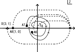
Figure 9: The motion of $A6,A7$ 7-branes along the path 1. Since the motion of $A8,D$ 7-branes are not relevant to the monodromy of this case, we do not write it in the figure.

When $a_{2}$ varies along the second path, the A6 7-brane’s position and the A7 7-brane’s position exchange with each other.

Next let us consider to rearrange the branch cuts of 7-branes before the exchange of A6 and A7 so that both 7-branes do not cross any branch cuts except for themselves’ during the exchange. This process is collected in the Table LABEL:tab:2-cycles_before_ex. It shows that the configuration of 7-branes and how the 2-cycles change by the above rearrangement.

Table 5: The motion of 7-branes and the changes of the 2-cycles along the path1.

A8[1,0] A7[1,0] A6[1,0] A5[1,0] A4-A1[1,0] B[1,-1] C1, C2[1,1] D[3,1] $C_{A65}$ 0 0 1 $-1$ 0 0 0 0 $C_{A76}$ 0 1 $-1$ 0 0 0 0 0 $C_{A87}$ 1 $-1$ 0 0 0 0 0 0 $C_{BCD}$ 0 0 0 0 0 1 1 $-1$

$\downarrow$ step 1

A6 and E6 go across the cut of A7 from right to left

A8[1,0] A6[1,0] A5[1,0] A4-A1[1,0] B[0,-1] C1, C2[2,1] A7[1,0] D[3,1] $C_{A65}$ 0 1 $-1$ 0 0 0 0 0 $C_{A76}$ 0 $-1$ 0 0 0 0 1 0 $C_{A87}$ 1 0 0 0 0 0 $-1$ 0 $C_{BCD}$ 0 0 0 0 1 1 0 $-1$

$\downarrow$ step 2

A7 goes across the cut of A6 and E6 from right to left.

A8[1,0] A7[3,1] A6[1,0] A5[1,0] A4-A1[1,0] B[0,-1] C1, C2[2,1] D[3,1] $C_{A65}$ 0 0 1 $-1$ 0 0 0 0 $C_{A76}$ 0 1 $-2$ $-1$ $-1$ 3 1 0 $C_{A87}$ 1 $-1$ 1 1 1 $-3$ $-1$ 0 $C_{BCD}$ 0 $-1$ 1 1 1 $-2$ 0 $-1$

$\downarrow$ step 3

A6 goes across the cut of E6 from left to right.

A8[1,0] A7[3,1] A5[1,0] A4-A1[1,0] B[0,-1] C1, C2[2,1] A6[-3,-1] D[3,1] $C_{A65}$ 0 0 $-1$ 0 1 1 1 0 $C_{A76}$ 0 1 $-1$ $-1$ 1 $-1$ $-2$ 0 $C_{A87}$ 1 $-1$ 1 1 $-2$ 0 1 0 $C_{BCD}$ 0 $-1$ 1 1 $-1$ 1 1 $-1$

$\downarrow$ step 4

E6 goes across the cut of A6 from left to right.

A8[1,0] A7[3,1] A6[-3,-1] A5[4,1] A4-A1[4,1] B[9,2] C1, C2[-1,0] D[3,1] $C_{A65}$ 0 0 1 $-1$ 0 1 1 0 $C_{A76}$ 0 1 $-2$ $-1$ $-1$ 1 $-1$ 0 $C_{A87}$ 1 $-1$ 0 1 1 $-2$ 0 0 $C_{BCD}$ 0 $-1$ 1 1 1 $-1$ 1 $-1$

After the step 4, A7’s position and A6’s position exchange with each other. Note that the A7 charge and the A6 charge are the same up to sign. Hence we do not need to rearrange the branch cuts in this exchange process. We get the Table LABEL:tab:after_ex after the exchange.

Table 6: The figure shows the motion of 7-branes during the path 2 and the table represents the changes of 2-cycles after the path 2

A8[1,0] A6[-3,-1] A7[3,1] A5[4,1] A4-A1[4,1] B[9,2] C1, C2[-1,0] D[3,1] $\tilde{C}_{A65}$ 0 1 0 $-1$ 0 1 1 0 $\tilde{C}_{A76}$ 0 $-2$ 1 $-1$ $-1$ 1 $-1$ 0 $\tilde{C}_{A87}$ 1 0 $-1$ 1 1 $-2$ 0 0 $\tilde{C}_{BCD}$ 0 1 $-1$ 1 1 $-1$ 1 $-1$

We follow the above 4 steps backward, then we get the second part of the Table LABEL:tab:back. The A6 charge and the A7 charge are $[-1,0]$. Since their charge is $[1,0]$ originally, we make their charges into the the original charges $[1,0]$. Then the second part of the Table LABEL:tab:back becomes last part of the Table LABEL:tab:back.

Table 7: The configurations of 7-branes and the changes of 2-cycles when we go 4 steps in the Table LABEL:tab:2-cycles_before_ex in a backward direction. The last part shows the change of the bases into the ones at the base point.

A8[1,0] A6[-3,-1] A7[3,1] A5[4,1] A4-A1[4,1] B[9,2] C1, C2[-1,0] D[3,1] $\tilde{C}_{A65}$ 0 1 0 $-1$ 0 1 1 0 $\tilde{C}_{A76}$ 0 $-2$ 1 $-1$ $-1$ 1 $-1$ 0 $\tilde{C}_{A87}$ 1 0 $-1$ 1 1 $-2$ 0 0 $\tilde{C}_{BCD}$ 0 1 $-1$ 1 1 $-1$ 1 $-1$

$\downarrow$

Going back the four steps of the Table LABEL:tab:2-cycles_before_ex

A8[1,0] A6[-1,0] A7[-1,0] A5[1,0] A4-A1[1,0] B[1,-1] C1, C2[1,1] D[3,1] $\tilde{C}_{A65}$ 0 1 1 $-2$ $-1$ 4 2 0 $\tilde{C}_{A76}$ 0 $-2$ $-1$ 1 1 $-4$ $-2$ 0 $\tilde{C}_{A87}$ 1 0 $-2$ 1 1 $-4$ $-2$ 0 $\tilde{C}_{BCD}$ 0 0 0 0 0 1 1 $-1$

$\downarrow$

Changing the bases into the ones before the rotation

A8[1,0] A6[1,0] A7[1,0] A5[1,0] A4-A1[1,0] B[1,-1] C1, C2[1,1] D[3,1] $\tilde{C}_{A65}$ 0 $-1$ $-1$ $-2$ $-1$ 4 2 0 $\tilde{C}_{A76}$ 0 2 1 1 1 $-4$ $-2$ 0 $\tilde{C}_{A87}$ 1 0 2 1 1 $-4$ $-2$ 0 $\tilde{C}_{BCD}$ 0 0 0 0 0 1 1 $-1$

From the first table of Table LABEL:tab:2-cycles_before_ex and the last table of the Table LABEL:tab:back, we get

$$\tilde{C}_{A65} =C_{-\theta}+C_{A65}+C_{A76}$$ (101)

$$\tilde{C}_{A76} =-C_{-\theta}$$ (102)

$$\tilde{C}_{-\theta} =-C_{A76}$$ (103)

$$\tilde{C}_{A87} =-C_{-\theta}-C_{A76}+C_{A87}\,.$$ (104)

where the equalities of the equations (101) $\sim$ (104) should be understood up to the boundaries of the 3-dimensional cells. Note that $C_{\alpha}^{1}$, $C_{\alpha}^{2}$, $C_{\beta}^{1}$ and $C_{\beta}^{2}$ , which are the outside of $E_{8}$ are invariant. On the other hand, this monodromy acts on the 2-cycles inside $E_{8}$ as the Weyl reflection by $C_{A76}+C_{-\theta}$.

A.2.4 The monodromy of the loop $\gamma_{0-4}$

When $a_{0}$ varies along the loop $\gamma_{0-4}$, the exchange of A7 and A8 only happens (see Figure 10).

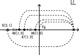
Figure 10: The left figure shows the motion of 7-branes when we approach the right of $a_{0}=a_{0-4}$ singularity. The right figure shows the motion of 7-brane when we go round $a_{0}=a_{0-4}$ singularity in an anti-clockwise direction.

Hence we get

$$\tilde{C}_{A76} =C_{A76}+C_{A87}$$ (105)

$$\tilde{C}_{A87} =-C_{A87}$$ (106)

$$\tilde{C}_{AA^{\prime}} =-C_{A87}+C_{AA^{\prime}}.$$ (107)

Note that $C_{A87}$ mixes into the 2-cycles inside $E_{8}$. This means that the monodromy of the loop $\gamma_{0-4}$ causes an effect beyond $E_{8}$ gauge theory.

$C_{\alpha}^{2}$ and $C_{\beta}^{2}$ do not mixes with $C_{\alpha}^{1}$, $C_{\beta}^{1}$ and the 2-cycles in $E_{8}$. We can understand this structure due to the $\epsilon_{\eta}$ scaling.

Appendix B Monodromy around $a_{0}=0$ Locus in Light of Heterotic Dual

It is instructive to see what the monodromy of 2-cycles (45–48) correspond to in Heterotic dual description. These monodromy matrices were obtained by a brute force calculation. Heterotic dual description tells us that this is a very natural result.

The duality map between F-theory and Heterotic string theory [42] is now well-understood. The moduli space of F-theory compactification on an elliptic K3 and that of Heterotic string compactification on $T^{2}$ are both $O(2)\times O(18)\backslash O(2,18;\mathbb{R})/O(2,18;\mathbb{Z})$. For the purpose of describing the action of the monodromy group $O(2,18;\mathbb{Z})$ explicitly, however, let us begin by reminding ourselves of the basic things about the duality map, while setting up notation.

The complex structure moduli of elliptic fibered K3 manifold for F-theory compactification is described (e.g., [41]) by 20 complex numbers $\Pi_{i}$ ($i=1,\cdots,20$) satisfying

$$\Pi_{i}C^{ij}\Pi_{j}=0,\qquad\Pi_{i}C^{ij}\Pi_{j}^{*}=2.$$ (108)

Multiplying an arbitrary complex phase on all the $\Pi_{i}$’s corresponds to the $O(2)$ redundancy of the moduli space. The moduli parameters $\Pi_{i}$ are obtained from a defining equation of an elliptic fibered K3 manifold as period integrals

$$\Pi_{i}=\int_{C_{i}}\Omega^{(2,0)}$$ (109)

of a holomorphic (2,0) form satisfying $\int_{K3}\Omega\wedge\overline{\Omega}=2$. $C^{ij}$ is the inverse matrix of the intersection form of 2-cycles of a K3 other than the zero section and the generic fiber class. We choose the first four 2-cycles to be $C_{\alpha}^{1}$, $C_{\alpha}^{2}$, $C_{\beta}^{1}$ and $C_{\beta}^{2}$ in this order, and use those in the first and last rows of Table 1 as the 16 other 2-cycles. For an elliptic fibered K3-manifold given by (11), for example,

$$\Pi_{C_{\alpha}^{1}}\sim\Pi_{C_{\beta}^{1}} \sim \frac{1}{\sqrt{\ln(1/\epsilon_{\eta})}},$$ (110)

$$\Pi_{C_{\alpha}^{2}}\sim\Pi_{C_{\beta}^{2}} \sim \sqrt{\ln(1/\epsilon_{\eta})},$$ (111)

$$\Pi_{C_{A76}}\sim\Pi_{C_{-\theta}}\sim\Pi_{C^{\prime}_{-\theta}} \sim \frac{1}{\sqrt{\ln(1/\epsilon_{\eta})}}\epsilon_{K}.$$ (112)

The Narain moduli of Heterotic string compactifications on a $T^{2}$ are described by 20 complex parameters

$$\Pi_{i}=\sqrt{\frac{\alpha^{\prime}}{2}}\left(k_{\hat{8}R}+ik_{\hat{9}R}\right)_{i}=\sqrt{\frac{\alpha^{\prime}}{2}}\frac{1}{\tau_{2}}(-i\tau k_{8R}+ik_{9R})_{i}$$ (113)

for $i=1,\cdots 20$; $(k_{mR})_{i}$ ($m=8,9$) above determine the momenta $k_{8R}$ and $k_{9R}$ in the right-moving sector by $k_{mR}=(k_{mR})_{i}n^{i}$, where $(n_{i})^{T}$ is a charge vector

$$(n^{i})^{T}=(n_{8},-w^{8},n_{9},-w^{9},n^{i=5,\cdots,20})^{T};$$ (114)

$(n_{8},n_{9})$ specify the Kaluza–Klein excitation level, and $(w^{8},w^{9})$ are the winding numbers. $n^{i}\in\mathbb{Z}$’s ($i=5,\cdots,20$) generate root lattice of $E_{8}\times E_{8}$. $k_{8R}$ and $k_{9R}$ are parametrized by 16 Wilson lines $(-i\tau A_{8}+iA_{9})^{i}\in\mathbb{C}$ ($i=5,\cdots,20$), complex structure $\tau=\tau_{1}+i\tau_{2}$ of the torus, $R$ and $B_{89}$; explicit expressions are found in (11.6.17) of [43].

With all the conventions fixed as above, the duality map is to identify $\Pi_{i}$’s of the two descriptions. One can see by comparing $\Pi_{i}$’s calculated on both sides that

$$\frac{R}{\sqrt{\alpha^{\prime}}}\quad({\rm Het})\leftrightarrow\sqrt{\ln(1/\epsilon_{\eta})}\quad({\rm F-theory}),$$ (115)

as is well known [20, 27], and

$$\frac{1}{\tau_{2}}R(-i\tau A_{8}+iA_{9})^{i}\quad({\rm Het})\leftrightarrow{\rm fcn}\left(\frac{a_{r}}{a_{0}}\right)\sim\epsilon_{K}\quad({\rm F-theory}),$$ (116)

where we assumed that $a_{0}$ may scale as $\epsilon_{\eta}$, but $a_{0,*}$ in (15, 16) remains ${\cal O}(1)$ and non-zero. Thus the choice of complex structure moduli with a small $\epsilon_{K}$ in (15) and $a_{0,*}\sim{\cal O}(1)$ in F-theory corresponds to Wilson lines in Heterotic string theory in $T^{2}$ that are parametrically smaller than the Kaluza–Klein scale of the $T^{2}$ compactification. Thus, the $T^{2}$ Kaluza–Klein states decouple and a gauge theory on 7+1 dimensions is obtained also in the Heterotic description. The “8D gauge theory region” of F-theory moduli space corresponds to 8D gauge theory on the Heterotic side.

Both F-theory compactified on an elliptic K3 manifold and Heterotic string theory compactified on $T^{2}$ have 20 U(1) vector fields on 7+1 dimensions. The charge vector $(n^{i})^{T}$ that appeared in (114) specifies charges of an object under these 20 U(1) vector fields. In the convention we adopted above, the last 16 U(1) vector fields are those in $E_{8}\times E_{8}$. In Heterotic string compactifications, the vector fields corresponding to the charges $n_{8,9}$ are Kaluza–Klein vector fields from the metric on 9+1 dimensions, and those to $w^{8,9}$ are those from the $B$-field. The monodromy group $O(2,18;\mathbb{Z})$ acts from the right on all of 2-cycles $(C_{i})$, moduli parameters $(\Pi_{i})$, and on 20 independent U(1) vector fields.

Having prepared all above, we are now ready to interpret the monodromy matrix (45) in Heterotic dual description. Since we considered monodromy in F-theory that appears even in $|\epsilon_{\eta}|\ll 1$, it must be a monodromy in Heterotic string theory that appear even in $R/\sqrt{\alpha^{\prime}}$, that is, in a region of moduli space where supergravity + super Yang–Mill approximation can be used. In particular, the compactification can be described in terms of Calabi–Yau 3-fold and a stable vector bundle on it. The bundle is described by a spectral surface. The spectral surface in the Heterotic dual [27, 44] is given by [45, 23, 2, 24, 4]

$$a_{0}+a_{2}x+a_{3}y+\cdots=0,$$ (117)

using the same coefficients $a_{0,2,3,\cdots}$ as in F-theory compactifications. $(x,y)$ are the coordinates of the elliptic fiber for the Heterotic string compactification. When $a_{0}\neq 0$ and $a_{r}/a_{0}\sim\epsilon_{K}^{r}$ for $r=2,3,\cdots$, the spectral surface is near the zero section. In a neighbourhood of a base manifold where $a_{0}$ becomes zero, however, two roots of (117) move away from the zero section, and behave as specified by (9), which indicates that a Weyl reflection takes place within $E_{8}$.

Noting that the monodromy matrix (46) can be decomposed into

$$\left(\begin{array}[]{cc|cc|c}1&&&&\\ &-1&&-1&\\ \hline\cr&2&1&1&\\ &&&1&\\ \hline\cr&&&&{\bf 1}_{2\times 2}\end{array}\right)=\left(\begin{array}[]{cc|cc|c}1&&&&\\ &-1&&&\\ \hline\cr&&1&&\\ &&&1&\\ \hline\cr&&&&{\bf 1}_{2\times 2}\end{array}\right)\left(\begin{array}[]{cc|cc|c}1&&&&\\ &1&&1&\\ \hline\cr&2&1&1&\\ &&&1&\\ \hline\cr&&&&{\bf 1}_{2\times 2}\end{array}\right);$$ (118)

here, we used a basis $(2C_{A76}+C_{-\theta},C_{-\theta},C_{\alpha}^{1},C_{\alpha}^{2},C_{\beta}^{1},C_{\beta}^{2})$, changing the first element of the basis from $C_{A76}$, so that the first two elements of this basis are dual to the Cartan elements $\mathop{\rm diag}\nolimits(2,-1,-1)$ and $\mathop{\rm diag}\nolimits(0,1,-1)$ acting on $(C_{A65},C_{A76}+C_{A65},C_{-\theta}+C_{A76}+C_{A65})$. The first matrix on the right hand side is $W_{C_{-\theta}}$, a Weyl reflection in $E_{8}$.

The second matrix above is not hard to understand, either. It is satisfactory that non-winding states ($w^{8,9}=0$) remain non-winding states; since we have chosen $|\epsilon_{\eta}|\ll 1$ and hence $R/\sqrt{\alpha^{\prime}}\gg 1$, supergravity / super Yang–Mills modes on 9+1 dimensions should not mix with winding states. When we take $|\epsilon_{K}|\ll 1$, the spectral surface scan the elliptic fiber once near a zero locus of $a_{0}$. This means that the Wilson line associated with the Weyl reflection varies by of order the Kaluza–Klein scale (i.e., $R(A_{\hat{8}}+iA_{\hat{9}})^{I}$ changes by ${\cal O}(1)$). This Wilson line is identified with the original one modulo gauge transformation whose parameter depends on the $T^{2}$ direction. Thus, the Kaluza–Klein excitation number $n_{8}$ (the 3rd row) becomes $\tilde{n_{8}}=n_{8}+2n^{-\theta}$ in this monodromy matrix. Once this coefficient $2$ is fixed, then there is no freedom left in the 4th column, because the intersection form needs to remain invariant.

This monodromy involves field identification modulo gauge transformation depending on the $T^{2}$ direction; there is no way describing this phenomenon in a gauge theory on 7+1 dimensions! This intuitive understanding of the monodromy matrix also explains why some U(1) symmetry charges within $E_{8}$ mix up with U(1) symmetries of Kaluza–Klein vector fields.

One would not bother about all these things when one considers, say, a Heterotic string compactification on a Calabi–Yau 3-fold with a vector bundle whose structure group is $\mathop{\rm SU}(5)_{\rm str}$. All the four U(1)’s in the Cartan of $\mathop{\rm SU}(5)_{\rm str}$ are broken completely, because of the ramification behavior of the spectral surface. All the four Kaluza–Klein vector fields from metric and $B$-field in 7+1 dimensions do not remain in the massless spectrum in 3+1 dimensions. Since none of those U(1) vector fields and U(1) symmetries available at microscopic level is relevant to low-energy physics, nobody cares how they are mixed up.

In the factorized spectral surface scenario in the context of dimension-4 proton decay problem, however, one wants to keep a U(1) symmetry out of a four independent U(1)’s in ${\rm SU}(5)_{\rm str}$. For this purpose, one has to make sure that at least one U(1) symmetry survives the monodromy that would potentially mix up all of U(1)’s in $E_{8}$ as well as those associated with Kaluza–Klein vector fields.

References

- [1] S. Katz and C. Vafa, “Matter From Geometry,” Nucl. Phys. B 497, 146 (1997) [arXiv:hep-th/9606086].
- [2] R. Donagi and M. Wijnholt, “Model Building with F-Theory,” arXiv:0802.2969 [hep-th].
- [3] C. Beasley, J. J. Heckman and C. Vafa, “GUTs and Exceptional Branes in F-theory - I,” JHEP 0901, 058 (2009) [arXiv:0802.3391 [hep-th]].
- [4] H. Hayashi, T. Kawano, R. Tatar and T. Watari, “Codimension-3 Singularities and Yukawa Couplings in F-theory,” Nucl. Phys. B 823, 47 (2009) [arXiv:0901.4941 [hep-th]].
- [5] R. Donagi and M. Wijnholt, “Higgs Bundles and UV Completion in F-Theory,” arXiv:0904.1218 [hep-th].
- [6] R. Tatar, Y. Tsuchiya and T. Watari, “Right-handed Neutrinos in F-theory Compactifications,” Nucl. Phys. B 823, 1 (2009) [arXiv:0905.2289 [hep-th]].
- [7] S. Cecotti, M. C. N. Cheng, J. J. Heckman and C. Vafa, “Yukawa Couplings in F-theory and Non-Commutative Geometry,” arXiv:0910.0477 [hep-th].
- [8] J. P. Conlon and E. Palti, “Aspects of Flavour and Supersymmetry in F-theory GUTs,” JHEP 1001, 029 (2010) [arXiv:0910.2413 [hep-th]].
- [9] Appendix of [31].
- [10] R. Tatar and T. Watari, “Proton decay, Yukawa couplings and underlying gauge symmetry in string theory,” Nucl. Phys. B 747, 212 (2006) [arXiv:hep-th/0602238].
- [11] J. Marsano, N. Saulina and S. Schafer-Nameki, “Monodromies, Fluxes, and Compact Three-Generation F-theory GUTs,” JHEP 0908, 046 (2009) [arXiv:0906.4672 [hep-th]].
- [12] C. Beasley, J. J. Heckman and C. Vafa, “GUTs and Exceptional Branes in F-theory - II: Experimental Predictions,” JHEP 0901, 059 (2009) arXiv:0806.0102 [hep-th].
- [13] R. Donagi and M. Wijnholt, “Breaking GUT Groups in F-Theory,” arXiv:0808.2223 [hep-th].
- [14] V. Bouchard, J. J. Heckman, J. Seo and C. Vafa, “F-theory and Neutrinos: Kaluza-Klein Dilution of Flavor Hierarchy,” JHEP 1001, 061 (2010) [arXiv:0904.1419 [hep-ph]].
- [15] J. J. Heckman, A. Tavanfar and C. Vafa, “The Point of in F-theory GUTs,” arXiv:0906.0581 [hep-th].
- [16] R. Blumenhagen, T. W. Grimm, B. Jurke and T. Weigand, “Global F-theory GUTs,” Nucl. Phys. B 829, 325 (2010) [arXiv:0908.1784 [hep-th]].
- [17] O. DeWolfe, T. Hauer, A. Iqbal and B. Zwiebach, “Uncovering infinite symmetries on (p,q) 7-branes: Kac-Moody algebras and beyond,” Adv. Theor. Math. Phys. 3, 1835 (1999) [arXiv:hep-th/9812209].
- [18] M. Bershadsky, K. A. Intriligator, S. Kachru, D. R. Morrison, V. Sadov and C. Vafa, “Geometric singularities and enhanced gauge symmetries,” Nucl. Phys. B 481, 215 (1996) [arXiv:hep-th/9605200].
- [19] S. Katz and D. R. Morrison, “ Gorenstein Threefold Singularities with Small Resolutions via Invariant Theory for Weyl Groups,” J. Alg. Geom. 1 (1992) 449–530 [arXiv:alg-geom/9202002].
- [20] D. R. Morrison and C. Vafa, “Compactifications of F-Theory on Calabi–Yau Threefolds – II,” Nucl. Phys. B 476, 437 (1996) [arXiv:hep-th/9603161].
- [21] K. Dasgupta, G. Rajesh and S. Sethi, “M Theory, Orientifolds and G-Flux,” JHEP 9908, 023 (1999) [arXiv:hep-th/9908088].
- [22] F. Cachazo, S. Katz and C. Vafa, “Geometric transitions and N = 1 quiver theories,” arXiv:hep-th/0108120.
- [23] G. Curio and R. Y. Donagi, “Moduli in N = 1 heterotic/F-theory duality,” Nucl. Phys. B 518 (1998) 603 [arXiv:hep-th/9801057].
- [24] H. Hayashi, R. Tatar, Y. Toda, T. Watari and M. Yamazaki, “New Aspects of Heterotic–F Theory Duality,” Nucl. Phys. B 806, 224 (2009) [arXiv:0805.1057 [hep-th]].
- [25] A. Johansen, “A comment on BPS states in F-theory in 8 dimensions,” Phys. Lett. B 395, 36 (1997) [arXiv:hep-th/9608186].
- [26] M. R. Gaberdiel and B. Zwiebach, “Exceptional groups from open strings,” Nucl. Phys. B 518, 151 (1998) [arXiv:hep-th/9709013].
- [27] R. Friedman, J. Morgan and E. Witten, “Vector bundles and F theory,” Commun. Math. Phys. 187 (1997) 679 [arXiv:hep-th/9701162].
- [28] J. Marsano, N. Saulina and S. Schafer-Nameki, “F-theory Compactifications for Supersymmetric GUTs,” JHEP 0908, 030 (2009) [arXiv:0904.3932 [hep-th]].
-
[29]
O. DeWolfe and B. Zwiebach,
“String junctions for arbitrary Lie algebra representations,”
Nucl. Phys. B 541, 509 (1999)
[arXiv:hep-th/9804210];
O. DeWolfe, T. Hauer, A. Iqbal and B. Zwiebach, “Uncovering the symmetries on (p,q) 7-branes: Beyond the Kodaira classification,” Adv. Theor. Math. Phys. 3, 1785 (1999) [arXiv:hep-th/9812028]. - [30] A. Klemm, B. Lian, S. S. Roan and S. T. Yau, “Calabi-Yau fourfolds for M- and F-theory compactifications,” Nucl. Phys. B 518, 515 (1998) [arXiv:hep-th/9701023].
- [31] H. Hayashi, T. Kawano, Y. Tsuchiya and T. Watari, “Flavor Structure in F-theory Compactifications,” arXiv:0910.2762 [hep-th].
- [32] C. Cordova, “Decoupling Gravity in F-Theory,” arXiv:0910.2955 [hep-th].
- [33] J. J. Heckman and C. Vafa, “Flavor Hierarchy From F-theory,” arXiv:0811.2417 v2 [hep-th].
- [34] F. Marchesano and L. Martucci, “Non-perturbative effects on seven-brane Yukawa couplings,” arXiv:0910.5496 [hep-th].
- [35] A. Font and L. E. Ibanez, “Matter wave functions and Yukawa couplings in F-theory Grand Unification,” JHEP 0909, 036 (2009) [arXiv:0907.4895 [hep-th]].
-
[36]
C. M. Chen and Y. C. Chung,
“A Note on Local GUT Models in F-Theory,”
Nucl. Phys. B 824, 273 (2010)
[arXiv:0903.3009 [hep-th]];
Y. C. Chung, “Abelian Gauge Fluxes and Local Models in F-Theory,” JHEP 1003, 006 (2010) [arXiv:0911.0427 [hep-th]]. - [37] J. L. Bourjaily, “Local Models in F-Theory and M-Theory with Three Generations,” arXiv:0901.3785 [hep-th].
- [38] F. Denef, “Les Houches Lectures on Constructing String Vacua,” arXiv:0803.1194 [hep-th].
- [39] J. H. Schwarz, “From Superstrings to M Theory,” Phys. Rept. 315 (1999) 107 [arXiv:hep-th/9807135].
- [40] M. R. Gaberdiel, T. Hauer and B. Zwiebach, “Open string-string junction transitions,” Nucl. Phys. B 525, 117 (1998) [arXiv:hep-th/9801205].
- [41] P. S. Aspinwall, “K3 Surfaces and String Duality,” arXiv:hep-th/9611137.
- [42] C. Vafa, “Evidence for F-Theory,” Nucl. Phys. B 469, 403 (1996) [arXiv:hep-th/9602022].
- [43] J. Polchinski, “String Theory,” Cambridge (1998).
-
[44]
R. Donagi, “Principal bundles on elliptic fibrations,”
Asian. J. Math 1 (1997) 214
[arXiv:alg-geom/9702002];
R. Donagi, “Taniguchi lecture on principal bundles on elliptic fibrations,” arXiv:hep-th/9802094. -
[45]
S. Katz, P. Mayr and C. Vafa,
“Mirror symmetry and exact solution of 4D N = 2 gauge theories. I,”
Adv. Theor. Math. Phys. 1, 53 (1998)
[arXiv:hep-th/9706110];
P. Berglund and P. Mayr, “Heterotic string/F-theory duality from mirror symmetry,” Adv. Theor. Math. Phys. 2, 1307 (1999) [arXiv:hep-th/9811217].