Practical Estimation of High Dimensional Stochastic Differential Mixed-Effects Models

Abstract

Stochastic differential equations (SDEs) are established tools to model physical phenomena whose dynamics are affected by random noise. By estimating parameters of an SDE intrinsic randomness of a system around its drift can be identified and separated from the drift itself. When it is of interest to model dynamics within a given population, i.e. to model simultaneously the performance of several experiments or subjects, mixed-effects modelling allows for the distinction of between and within experiment variability. A framework to model dynamics within a population using SDEs is proposed, representing simultaneously several sources of variation: variability between experiments using a mixed-effects approach and stochasticity in the individual dynamics using SDEs. These stochastic differential mixed-effects models have applications in e.g. pharmacokinetics/pharmacodynamics and biomedical modelling. A parameter estimation method is proposed and computational guidelines for an efficient implementation are given. Finally the method is evaluated using simulations from standard models like the two-dimensional Ornstein-Uhlenbeck (OU) and the square root models.

1 INTRODUCTION

Models defined through stochastic differential equations (SDEs) allow for the representation of random variability in dynamical systems. This class of models is becoming more and more important (e.g. Allen (2007) and Øksendal (2007)) and is a standard tool to model financial, neuronal and population growth dynamics. However, much has still to be done, both from a theoretical and from a computational point of view, to make it applicable in those statistical fields that are already well established for deterministic dynamical models (ODE, DDE, PDE). For example, studies in which repeated measurements are taken on a series of individuals or experimental units play an important role in biomedical research: it is often reasonable to assume that responses follow the same model form for all experimental subjects, but parameters vary randomly among individuals. The importance of these mixed-effects models (e.g. McCulloch and Searle (2001), Pinheiro and Bates (2002)) lies in their ability to split the total variation into within- and between-individual components.

The SDE approach has only recently been combined with mixed-effects models, because of the difficulties arising both from the theoretical and the computational side when dealing with SDEs. In Overgaard et al. (2005) and Tornøe et al. (2005) a stochastic differential mixed-effects model (SDMEM) with log-normally distributed random parameters and a constant diffusion term is estimated via (extended) Kalman filter. Donnet and Samson (2008) developed an estimation method based on a stochastic EM algorithm for fitting one-dimensional SDEs with mixed-effects. In Donnet et al. (2010) a Bayesian approach is applied to a one-dimensional model for growth curve data. The methods presented in the aforementioned references are computationally demanding when the dimension of the model and/or parameter space grows. However, they are all able to handle data contaminated by measurement noise. In Ditlevsen and De Gaetano (2005) the likelihood function for a simple SDMEM with normally distributed random parameters is calculated explicitly, but generally the likelihood function is unavailable. In Picchini et al. (2010) a computationally efficient method for estimating SDMEMs with random parameters following any sufficiently well-behaved continuous distribution was developed. First the conditional transition density of the diffusion process given the random effects is approximated in closed-form by a Hermite expansion, and then the obtained conditional likelihood is numerically integrated with respect to the random effects using Gaussian quadrature. The method resulted to be statistically accurate and computationally fast. However, in practice it was limited to one random effect only (see Picchini et al. (2008) for an application in neuroscience) since Gaussian quadrature is computationally inefficient when the number of random effects grows.

Here the method presented in Picchini et al. (2010) is extended to handle SDMEMs with multiple random effects. Furthermore, the application is extended in a second direction to handle multidimensional SDMEMs. Computational guidelines for a practical implementation are given, using e.g. automatic differentiation (AD) tools. Results obtained from simulation studies show that, at least for the examples discussed in the present work, the methodology is flexible enough to accommodate complex models having different distributions for the random effects, not only the normal or log-normal distributions which are the ones usually employed. Satisfactory estimates for the unknown parameters are obtained even considering small populations of subjects (i.e. few repetitions of an experiment) and few observations per subject/experiment, which is often relevant, especially in biomedicine where large data sets are typically unavailable.

A drawback of our approach is that measurement error is not accounted for, and thus it is most useful in those situations where the variance of the measurement noise is small compared to the system noise.

The paper is organized as follows. Section 2 introduces the SDMEMs, the observation scheme and the necessary notation. Section 3 introduces the likelihood function. Section 4 considers approximate methods for when the expression of the exact likelihood function cannot be obtained; computational guidelines and software tools are also discussed. Section 5 is devoted to the application on simulated datasets. Section 6 summarizes the results and the advantages and limitations of the method are discussed. An Appendix containing technical results closes the paper.

2 STOCHASTIC DIFFERENTIAL MIXED EFFECTS MODELS

In the following, bold characters are used to denote vectors and matrices. Consider a $d$-dimensional (Itô) SDE model for some continuous process $\mathbf{X}_{t}$ evolving in $M$ different experimental units randomly chosen from a theoretical population:

$$d\mathbf{X}_{t}^{i}=\boldsymbol{\mu}(\mathbf{X}_{t}^{i},{\boldsymbol{\theta}},\mathbf{b}^{i})dt+\boldsymbol{\sigma}(\mathbf{X}_{t}^{i},{\boldsymbol{\theta}},{\mathbf{b}}^{i})\,d\mathbf{W}_{t}^{i},\qquad\mathbf{X}_{0}^{i}=\mathbf{x}_{0}^{i},\qquad i=1,\ldots,M$$ (1)

where $\mathbf{X}_{t}^{i}$ is the value at time $t\geq t_{0}^{i}$ of the $i$th unit, with $\mathbf{X}_{0}^{i}=\mathbf{X}_{t_{0}^{i}}^{i}$; $\boldsymbol{\theta}\in\boldsymbol{\Theta}\subseteq\mathbb{R}^{p}$ is a $p$-dimensional fixed effects parameter (the same for the entire population) and $\mathbf{b}^{i}\equiv\mathbf{b}^{i}(\boldsymbol{\Psi})\in B\subseteq\mathbb{R}^{q}$ is a $q$-dimensional random effects parameter (unit specific) with components $(b_{1}^{i},...,b_{q}^{i})$; each component $b^{i}_{l}$ may follow a different continuous distribution ($l=1,...,q$). Let $p_{B}(\mathbf{b}^{i}|\boldsymbol{\Psi})$ denote the joint distribution of the vector $\mathbf{b}^{i}$, parametrized by an $r$-dimensional parameter $\boldsymbol{\Psi}\in\Upsilon\subseteq\mathbb{R}^{r}$. The $\mathbf{W}_{t}^{i}$’s are $d$-dimensional standard Brownian motions with components $W_{t}^{(h)i}$ ($h=1,...,d$). The $W_{t}^{(h)i}$ and ${b}^{j}_{l}$ are assumed mutually independent for all $1\leq i,j\leq M$, $1\leq h\leq d$, $1\leq l\leq q$. The initial condition $\mathbf{X}_{0}^{i}$ is assumed equal to a vector of constants $\mathbf{x}_{0}^{i}\in\mathbb{R}^{d}$. The drift and the diffusion coefficient functions $\boldsymbol{\mu}(\cdot):E\times\Theta\times B\rightarrow\mathbb{R}^{d}$ and $\boldsymbol{\sigma}(\cdot):E\times\Theta\times B\rightarrow\mathbb{S}$ are assumed known up to the parameters, and are assumed sufficiently regular to ensure a unique weak solution (Øksendal (2007)), where $E\subseteq\mathbb{R}^{d}$ denotes the state space of $\mathbf{X}^{i}_{t}$ and $\mathbb{S}$ denotes the set of $d\times d$ positive definite matrices. Model (1) assumes that in each of the $M$ units the evolution of $\mathbf{X}$ follows a common functional form, and therefore differences between units are due to different realizations of the Brownian motion paths $\{\mathbf{W}_{t}^{i}\}_{t\geq t_{0}^{i}}$ and of the random parameters $\mathbf{b}^{i}$. Thus, the dynamics within a generic unit $i$ are expressed via an SDE model driven by Brownian motion, and the introduction of a vector parameter randomly varying among units allows for the explanation of the variability between the $M$ units.

Assume that the distribution of $\mathbf{X}_{t}^{i}$ given $(\mathbf{b}^{i},\boldsymbol{\theta})$ and $\mathbf{X}_{s}^{i}=\mathbf{x}_{s},$ $s<t$, has a strictly positive density w.r.t. the Lebesgue measure on $E$, which is denoted by

$$\mathbf{x}\rightarrow p_{X}(\mathbf{x},t-s|\mathbf{x}_{s},\boldsymbol{b}^{i},\boldsymbol{\theta})>0,\hskip 5.69054pt\mathbf{x}\in E.$$ (2)

Assume moreover that unit $i$ is observed at the same set of $n_{i}+1$ discrete time points $\{t_{0}^{i},t_{1}^{i},\ldots,t_{n_{i}}^{i}\}$ for each coordinate $X_{t}^{(h)i}$ of the process $\mathbf{X}_{t}^{i}$ ($h=1,...,d$), whereas different units may be observed at different sets of time points. Let $\mathbf{x}^{i}$ be the $(n_{i}+1)\times d$ matrix of responses for unit $i$, with $j$th row given by $\mathbf{x}^{i}(t_{j}^{i})=\mathbf{x}^{i}_{j}=(x^{(1)i}_{j},...,x^{(d)i}_{j})$, and let the following be the $N\times d$ total response matrix, $N=\sum_{i=1}^{M}(n_{i}+1)$:

$$\mathbf{x}=({\mathbf{x}^{1}}^{T},...,{\mathbf{x}^{M}}^{T})^{T}=\left(\begin{array}[]{ccc}x_{0}^{(1)1}&\cdots&x_{0}^{(d)1}\\ \vdots&\vdots&\vdots\\ x_{n_{1}}^{(1)1}&\cdots&x_{n_{1}}^{(d)1}\\ \vdots&\vdots&\vdots\\ x^{(1)i}_{j}&\cdots&x^{(d)i}_{j}\\ \vdots&\vdots&\vdots\\ x_{0}^{(1)M}&\cdots&x_{0}^{(d)M}\\ \vdots&\vdots&\vdots\\ x_{n_{M}}^{(1)M}&\cdots&x_{n_{M}}^{(d)M}\\ \end{array}\right),$$

where $T$ denotes transposition. Write $\Delta_{j}^{i}=t_{j}^{i}-t_{j-1}^{i}$ for the time distance between $\mathbf{x}_{j-1}^{i}$ and $\mathbf{x}_{j}^{i}$. Notice that this observation scheme implies that the matrix of data $\mathbf{x}$ must not contain missing values.

The goal is to estimate $(\boldsymbol{\theta,\Psi})$ using simultaneously all the data in $\mathbf{x}$. The specific values of the $\boldsymbol{b}^{i}$’s are not of interest, but only the identification of the vector-parameter $\boldsymbol{\Psi}$ characterizing their distribution. However, estimates of the random parameters $\boldsymbol{b}^{i}$ are also obtained, since it is necessary to estimate them when estimating $(\boldsymbol{\theta,\Psi})$.

3 MAXIMUM LIKELIHOOD ESTIMATION

To obtain the marginal density of $\mathbf{x}^{i}$, the conditional density of the data given the non-observable random effects $\mathbf{b}^{i}$ is integrated with respect to the marginal density of the random effects, using that $W_{t}^{(h)i}$ and ${b}^{j}_{l}$ are independent. This yields the likelihood function

$$L(\boldsymbol{\theta,\Psi}) = \prod_{i=1}^{M}p({\mathbf{x}^{i}}|\boldsymbol{\theta,\Psi})\,=\,\prod_{i=1}^{M}\int_{B}p_{\underline{X}}({\mathbf{x}^{i}}|\mathbf{b}^{i},\boldsymbol{\theta})\,p_{B}(\mathbf{b}^{i}|\boldsymbol{\Psi})\,d\mathbf{b}^{i}.$$ (3)

Here $p(\cdot)$ is the density of $\mathbf{x}^{i}$ given $(\boldsymbol{\theta,\Psi})$, $p_{B}(\cdot)$ is the density of the random effects, and $p_{\underline{X}}(\cdot)$ is the product of the transition densities $p_{X}(\cdot)$ given in (2) for a given realization of the random effects and for a given $\boldsymbol{\theta}$,

$$p_{\underline{X}}(\mathbf{x}^{i}|\mathbf{b}^{i},\boldsymbol{\theta}) = \prod_{j=1}^{n_{i}}p_{X}(\mathbf{x}^{i}_{j},\Delta_{j}^{i}|\mathbf{x}^{i}_{j-1},\mathbf{b}^{i},\boldsymbol{\theta}).$$ (4)

In applications the random effects are often assumed to be (multi)normally distributed, but $p_{B}(\cdot)$ could be any well-behaved density function. Solving the integral in (3) yields the marginal likelihood of the parameters for unit $i$, independent of the random effects $\mathbf{b}^{i}$; by maximizing the resulting expression (3) with respect to $\boldsymbol{\theta}$ and $\boldsymbol{\Psi}$ the corresponding maximum likelihood estimators (MLE) $\hat{\boldsymbol{\theta}}$ and $\hat{\boldsymbol{\Psi}}$ are obtained. Notice that it is possible to consider random effects having discrete distributions: in that case the integral becomes a sum and can be easily computed when the transition density $p_{X}$ is known. In this paper only random effects having continuous distributions are considered.

In simple cases an explicit expression for the likelihood function, and even explicit estimating equations for the MLEs can be found (Ditlevsen and De Gaetano (2005)). However, in general it is not possible to find an explicit solution for the integral, and thus exact MLEs are unavailable. This occurs when: (i) $p_{X}(\mathbf{x}_{j}^{i},\cdot|\mathbf{x}_{j-1}^{i},\cdot)$ is known but it is not possible to analytically solve the integral, and (ii) $p_{X}(\mathbf{x}_{j}^{i},\cdot|\mathbf{x}_{j-1}^{i},\cdot)$ is unknown. In (i) the integral must be evaluated numerically to obtain an approximation of the likelihood (3). In (ii) first $p_{X}(\mathbf{x}_{j}^{i},\cdot|\mathbf{x}_{j-1}^{i},\cdot)$ is approximated, then the integral in (3) is solved numerically.

In situation (ii) there exist several strategies to approximate the density $p_{X}(\mathbf{x}_{j}^{i},\cdot|\mathbf{x}_{j-1}^{i},\cdot)$, e.g. Monte Carlo approximations, direct solution of the Fokker-Planck equation, or Hermite expansions, just to mention some of the possible approaches, see Hurn et al. (2007) for a comprehensive review focused on one-dimensional diffusions. We propose to approximate the transition density in closed-form using a Hermite expansion (Aït-Sahalia (2008)). It often provides a good approximation to $p_{X}$, and Jensen and Poulsen (2002) showed that the method is computationally efficient. Using the obtained expression, the likelihood function is approximated, thus deriving approximated MLEs of $\boldsymbol{\theta}$ and $\boldsymbol{\Psi}$.

4 CLOSED-FORM TRANSITION DENSITY EXPANSION AND LIKELIHOOD APPROXIMATION

4.1 Transition Density Expansion for Multidimensional SDEs

Here the transition density expansion of a $d$-dimensional time-homogeneous SDE as suggested in Aït-Sahalia (2008) is reviewed; the same reference provides a method to handle multi-dimensional time-inhomogeneous SDEs, but for ease of exposition attention is focused on the former case. Also references on further extensions, e.g. Lévy processes, are given in the paper. We will only consider SDEs reducible to unit diffusion, i.e. multi-dimensional diffusions $\mathbf{X}$ for which there exists a one-to-one transformation to another diffusion with diffusion matrix the identity matrix. It is possible to perform the density expansion also for non-reducible SDEs (Aït-Sahalia (2008)). For the moment reference to $\boldsymbol{\theta}$ is dropped when not necessary, i.e. a function $f(x,\boldsymbol{\theta})$ is written $f(x)$.

Consider the following $d$-dimensional, reducible, time-homogeneous SDE

$$d\mathbf{X}_{t}=\boldsymbol{\mu}(\mathbf{X}_{t})dt+\boldsymbol{\sigma}(\mathbf{X}_{t})d\mathbf{W}_{t},\qquad\mathbf{X}_{0}=\mathbf{x}_{0}$$ (5)

and a series of $d$-dimensional discrete observations $\mathbf{x}_{0},\mathbf{x}_{1},...,\mathbf{x}_{n}$ from $\mathbf{X}$, all observed at the same time points $\{t_{0},t_{1},...,t_{n}\}$; denote with $E$ the state space of $\mathbf{X}$. We want to approximate $p_{X}(\mathbf{x}_{j},\Delta_{j}|\mathbf{x}_{j-1})$, the conditional density of $\mathbf{X}_{j}$ given $\mathbf{X}_{j-1}=\mathbf{x}_{j-1}$, where $\Delta_{j}=t_{j}-t_{j-1}$ ($j=1,...,n$). Under regularity conditions (e.g. $\boldsymbol{\mu}(\mathbf{x})$ and $\boldsymbol{\sigma}(\mathbf{x})$ are assumed to be infinitely differentiable in $\mathbf{x}$ on $E$, $\mathbf{v}(\mathbf{x}):=\boldsymbol{\sigma}(\mathbf{x})\boldsymbol{\sigma}(\mathbf{x})^{T}$ is a $d\times d$ positive definite matrix for all $\mathbf{x}$ in the interior of $E$ and all the drift and diffusion components satisfy linear growth conditions, see Aït-Sahalia (2008) for details), the logarithm of the transition density can be expanded in closed form using an order $J=+\infty$ Hermite series, and approximated by a Taylor expansion up to order $K$,

$$\ln p_{X}^{(K)}(\mathbf{x}_{j},\Delta_{j}|\mathbf{x}_{j-1}) = -\frac{d}{2}\ln(2\pi\Delta_{j})-\frac{1}{2}\ln(\det(\mathbf{v}(\mathbf{x}_{j})))+\frac{C_{Y}^{(-1)}(\boldsymbol{\gamma}(\mathbf{x}_{j})|\boldsymbol{\gamma}(\mathbf{x}_{j-1}))}{\Delta_{j}}$$ (6)

$$+ \sum_{k=0}^{K}C_{Y}^{(k)}(\boldsymbol{\gamma}(\mathbf{x}_{j})|\boldsymbol{\gamma}(\mathbf{x}_{j-1}))\frac{\Delta^{k}_{j}}{k!}.$$

Here $\Delta_{j}^{k}$ denotes $\Delta_{j}$ raised to the power of $k$. The coefficients $C_{Y}^{(k)}$ are given in the Appendix and $\boldsymbol{\gamma}(\mathbf{x})=(\gamma^{(1)}(\mathbf{x}),...,\gamma^{(d)}(\mathbf{x}))^{T}$ is the Lamperti transform, which by definition exists when the diffusion is reducible, and is such that $\triangledown\boldsymbol{\gamma}(\mathbf{x})=\boldsymbol{\sigma}^{-1}(\mathbf{x})$. See the Appendix for a sufficient and necessary condition for reducibility. Using Itô’s lemma, the transformation $\mathbf{Y}_{t}=\boldsymbol{\gamma}(\mathbf{X}_{t})$ defines a new diffusion process $\mathbf{Y}_{t}$, solution of the following SDE

$$d\mathbf{Y}_{t}=\boldsymbol{\mu}_{Y}(\mathbf{Y}_{t})dt+d\mathbf{W}_{t},\qquad\mathbf{Y}_{0} = \mathbf{y}_{0},$$

where the $h$-th element of $\boldsymbol{\mu}_{Y}$ is given by ($h=1,...,d$)

$$\mu_{Y}^{(h)}(\mathbf{Y}_{t}) = \sum_{i=1}^{d}\biggl{(}\bigl{\{}\boldsymbol{\sigma}^{-1}({\boldsymbol{\gamma}}^{-1}(\mathbf{Y}_{t}))\bigr{\}}_{hi}\boldsymbol{\mu}^{(i)}({\boldsymbol{\gamma}}^{-1}(\mathbf{Y}_{t}))\biggr{)}$$

$$- \frac{1}{2}\sum_{i,j,k}^{d}\biggl{\{}\boldsymbol{\sigma}^{-1}({\boldsymbol{\gamma}}^{-1}(\mathbf{Y}_{t}))\frac{\partial\boldsymbol{\sigma}}{\partial x_{j}}(\boldsymbol{\gamma}^{-1}(\mathbf{Y}_{t}))\boldsymbol{\sigma}^{-1}({\boldsymbol{\gamma}}^{-1}(\mathbf{Y}_{t}))\biggr{\}}_{hi}\sigma_{ik}({\boldsymbol{\gamma}}^{-1}(\mathbf{Y}_{t}))\sigma_{jk}({\boldsymbol{\gamma}}^{-1}(\mathbf{Y}_{t})).$$

For ease of interpretation the Lamperti transform and the drift term $\mu_{Y}$ for a scalar ($d=1$) SDE are reported. Namely $\gamma(\cdot)$ is defined by

$$Y_{t}\equiv\gamma(X_{t})=\int^{X_{t}}\frac{du}{\sigma(u)},$$

where the lower bound of integration is an arbitrary point in the interior of $E$. The drift term is given by

$$\mu_{Y}(Y_{t})=\frac{\mu(\gamma^{-1}(Y_{t}))}{\sigma(\gamma^{-1}(Y_{t}))}-\frac{1}{2}\frac{\partial\sigma}{\partial x}(\gamma^{-1}(Y_{t})).$$

The transformation of $\mathbf{X}_{t}$ into $\mathbf{Y}_{t}$ is a necessary step to make the transition density of the transformed process closer to a normal distribution, so that the Hermite expansion gives reasonable results. However, the reader is warned that this is by no means an easy task for many multivariate SDEs, and impossible for those having non-reducible diffusion (see Aït-Sahalia (2008) for details). The use of a software with symbolic algebra capabilities like e.g. Mathematica, Maple or Maxima is necessary to carry out the calculations.

4.2 Likelihood Approximation and Parameter Estimation

For a reducible time-homogeneous SDMEM, the coefficients $C_{Y}^{(k)}$ are obtained as in Section 4.1 by taking $(\boldsymbol{\theta},\mathbf{b}^{i})$, $\Delta_{j}^{i}$ and $(\mathbf{x}^{i}_{j},\mathbf{x}^{i}_{j-1})$ instead of $\boldsymbol{\theta}$, $\Delta_{j}$ and $(\mathbf{x}_{j},\mathbf{x}_{j-1})$, respectively. Then $p_{X}^{(K)}$ is substituted for the unknown transition density in (4), thus obtaining a sequence of approximations to the likelihood function

$$L^{(K)}(\boldsymbol{\theta,\Psi})=\prod_{i=1}^{M}\int_{B}p_{\underline{X}}^{(K)}({\mathbf{x}^{i}}|\mathbf{b}^{i},\boldsymbol{\theta})\,p_{B}(\mathbf{b}^{i}|\boldsymbol{\Psi})\,d\mathbf{b}^{i},$$ (7)

where

$$p_{\underline{X}}^{(K)}(\mathbf{x}^{i}|\mathbf{b}^{i},\boldsymbol{\theta}) = \prod_{j=1}^{n_{i}}p_{X}^{(K)}(\mathbf{x}^{i}_{j},\Delta_{j}^{i}|\mathbf{x}^{i}_{j-1},\mathbf{b}^{i},\boldsymbol{\theta})$$ (8)

and $p_{X}^{(K)}$ is given by equation (6). By maximizing (7) with respect to $(\boldsymbol{\theta,\Psi})$, approximated MLEs $\boldsymbol{\hat{\theta}}^{(K)}$ and $\boldsymbol{\hat{\Psi}}^{(K)}$ are obtained.

In general, the integral in (7) does not have a closed form solution, and therefore efficient numerical integration methods are needed; see Picchini et al. (2010) for the case of a single random effect ($q=1$). General purpose approximation methods for one- or multi-dimensional integrals, irrespective of the random effects distribution, are available (e.g. Krommer and Ueberhuber (1998)) and implemented in several software packages, though the complexity of the problem grows fast when increasing the dimension of $B$. However, since exact transition densities or a closed-form approximation to $p_{X}$ are supposed to be available, analytic expressions for the integrands in (3) or (7) are known and the Laplace method (e.g. Shun and McCullagh (1995)) may be used. Write $\mathbf{b}^{i}=(b^{i}_{1},...,b^{i}_{q})$ and define

$$f(\mathbf{b}^{i}|\boldsymbol{\theta,\Psi})=\log p_{\underline{X}}({\mathbf{x}^{i}}|\mathbf{b}^{i},\boldsymbol{\theta})+\log p_{B}(\mathbf{b}^{i}|\boldsymbol{\Psi}),$$ (9)

where $p_{\underline{X}}({\mathbf{x}^{i}}|\mathbf{b}^{i},\boldsymbol{\theta})$ is given in (4). Then $\log\int_{B}e^{f(\mathbf{b}^{i}|\boldsymbol{\theta,\Psi})}d\mathbf{b}^{i}$ can be approximated using a second order Taylor series expansion, known as Laplace approximation:

$$\log\int_{B}e^{f(\mathbf{b}^{i}|\boldsymbol{\theta,\Psi})}d\mathbf{b}^{i}\simeq f(\hat{\mathbf{b}}^{i}|\boldsymbol{\theta,\Psi})+\frac{q}{2}\log(2\pi)-\frac{1}{2}\log\left|-\mathbf{H}(\hat{\mathbf{b}}^{i}|\boldsymbol{\theta,\Psi})\right|$$

where $\hat{\mathbf{b}}^{i}=\arg\max_{\mathbf{b}^{i}}f(\mathbf{b}^{i}|\boldsymbol{\theta,\Psi})$, and $\mathbf{H}(\mathbf{b}^{i}|\boldsymbol{\theta,\Psi})=\partial^{2}f(\mathbf{b}^{i}|\boldsymbol{\theta,\Psi})/\partial\mathbf{b}^{i}\partial{\mathbf{b}^{i}}^{T}$ is the Hessian of $f$ w.r.t. $\mathbf{b}^{i}$. Thus, the log-likelihood function is approximately given by

$$\log L(\boldsymbol{\theta,\Psi})\simeq\sum_{i=1}^{M}\biggl{[}f(\hat{\mathbf{b}}^{i}|\boldsymbol{\theta,\Psi})+\frac{q}{2}\log(2\pi)-\frac{1}{2}\log\left|-\mathbf{H}(\hat{\mathbf{b}}^{i}|\boldsymbol{\theta,\Psi})\right|\biggr{]}$$ (10)

and the values of $\boldsymbol{\theta}$ and $\boldsymbol{\Psi}$ maximizing (10) are approximated MLEs. For the special case where $-f(\mathbf{b}^{i}|\boldsymbol{\theta,\Psi})$ is quadratic and convex in $\mathbf{b}^{i}$ the Laplace approximation is exact (Joe (2008)) and (10) provides the exact likelihood function. An approximation of $\log L^{(K)}(\boldsymbol{\theta,\Psi})$ can be derived in the same way, and we denote with

$$(\boldsymbol{\hat{\theta}}^{(K)},\boldsymbol{\hat{\Psi}}^{(K)})=\arg\min_{\boldsymbol{\theta}\in\Theta,\boldsymbol{\Psi}\in\Upsilon}-\log L^{(K)}(\boldsymbol{\theta,\Psi})$$

the corresponding approximated MLE of $(\boldsymbol{\theta,\Psi})$. Davidian and Giltinan (2003) recommend to use the Laplace approximation only if $n_{i}$ is “large”; however Ko and Davidian (2000) note that even if the $n_{i}$’s are small, the inferences should still be valid if the magnitude of intra-individual variation is small relative to the inter-individual variation. This happens in many applications, e.g. in pharmacokinetics.

In general, computing (10) or $\log L^{(K)}(\boldsymbol{\theta,\Psi})$ is non-trivial, since $M$ independent optimization procedures must be run to obtain the $\hat{\mathbf{b}}^{i}$’s and then the $M$ Hessians $\mathbf{H}(\hat{\mathbf{b}}^{i}|\boldsymbol{\theta,\Psi})$ must be computed. The latter problem can be solved using either (i) approximations based on finite differences, (ii) computing the analytic expressions of the Hessians using a symbolic calculus program or (iii) using automatic differentiation tools (AD, e.g. Griewank (2000)). We recommend to avoid method (i) since it is computationally costly when the dimension of $M$ and/or $\mathbf{b}^{i}$ grows, whereas methods (ii)-(iii) are reliable choices, since symbolic packages are becoming standard in most software and are anyway necessary to calculate an approximation $p_{X}^{(K)}$ to the transition density. However, when a symbolic package is not available to the user or is not of help in some specific situations, AD can be a convenient (if not the only possible) choice, especially when the function to be differentiated is defined via a complex software code; see the Conclusion for a discussion.

In order to derive the required Hessian automatically we used the AD tool ADiMat for Matlab (Bischof et al. (2005)), see http://www.autodiff.org for a comprehensive list of other AD software. For example, assume that a user defined Matlab function named loglik_indiv computes the $f$ function in (9) at a given value of the random effects $\mathbf{b}^{i}$ (named b_rand):

   result = loglik_indiv(b_rand)

so result contains the value of $f$ at $\mathbf{b}^{i}$. The following Matlab code then invokes ADiMat and creates automatically a file named g_loglik_indiv containing the code necessary to return the exact (to machine precision) Hessian of loglik_indiv w.r.t. b_rand:

   addiff(@loglik_indiv, ’b_rand’,[], ’--2ndorderfwd’)

At this point we initialize the array and the matrix that will contain the gradient and the Hessian of $f$ w.r.t. the $q$-dimensional vector $\mathbf{b}^{i}$:

   gradient = createFullGradients(b_rand);  % inizialize the gradient
   Hessian = createHessians([q q], b_rand); % inizialize the Hessian
   [Hessian, gradient] = g_loglik_indiv(Hessian, gradient, b_rand);

The last line returns the desired Hessian and the gradient of $f$ evaluated at b_rand. We used the Hessian either to compute the Laplace approximation or in the trust region method used for the internal step optimization, read below. When it is possible to derive the expression for the Hessian analytically we strongly recommend to avoid the use of AD tools in order to speed up the estimation algorithm. For example, in Section 5.1 only two random effects are considered and using the Matlab Symbolic Calculus Toolbox we have obtained the analytic expression for the Hessian without much effort.

For the remainder of this Section the reference to the index $K$ is dropped, except where necessary, as the following apply irrespectively of whether $p_{X}$ or $p_{X}^{(K)}$ is used. The minimization of $-\log L(\boldsymbol{\theta},\boldsymbol{\Psi})$ is a nested optimization problem. First the internal optimization step estimates the $\hat{\mathbf{b}}^{i}$’s for every unit (the $\hat{\mathbf{b}}^{i}$’s are sometimes known in the literature as empirical Bayes estimators). Since both symbolic calculus and AD tools provide exact results for the derivatives of $f(\mathbf{b}^{i})$, the values provided via AD being only limited by the computer precision, the exact gradient and Hessian of $f(\mathbf{b}^{i})$ can be used to minimize $-f(\mathbf{b}^{i})$ w.r.t. $\mathbf{b}^{i}$. We used the subspace trust-region method described in Coleman and Li (1996) and implemented in the Matlab fminunc function. The external optimization step minimizes $-\log L(\boldsymbol{\theta,\Psi})$ w.r.t. $(\boldsymbol{\theta,\Psi})$, after plugging the $\hat{\mathbf{b}}^{i}$’s into (10). This is a computationally heavy task, especially for large $M$, because the $M$ internal optimization steps must be performed for each infinitesimal variation of the parameters $(\boldsymbol{\theta,\Psi})$. Therefore to perform the external step we reverted to derivative-free optimization methods, namely the Nelder-Mead simplex with additional checks on parameter bounds, as implemented by D’Errico (2006) for Matlab. To speed up the algorithm convergence, $\hat{\mathbf{b}}^{i}(k)$ may be used as starting value for $\mathbf{b}^{i}$ in the $(k+1)$th iteration of the internal step, where $\hat{\mathbf{b}}^{i}(k)$ is the estimate of $\mathbf{b}^{i}$ at the end of the $k$th iteration of the internal step. This might not be an optimal strategy, however it should improve over the choice made by some authors who use a vector of zeros as starting value for $\mathbf{b}^{i}$ each time the internal step is performed. The latter strategy may be inefficient when dealing with highly time consuming problems, as it requires many more iterations.

Once estimates for $\boldsymbol{\theta}$ and $\boldsymbol{\Psi}$ are available, estimates of the random parameters $\mathbf{b}^{i}$ are automatically given by the values of the $\mathbf{\hat{b}}^{i}$ at the last iteration of the external optimization step, see Section 5.2 for an example.

5 SIMULATION STUDIES

In this Section the efficacy of the method is assessed through Monte Carlo simulations under different experimental designs. We always choose $M$ and $n$ to be not very large, since in most applications, e.g. in the biomedical context, large datasets are often unavailable. However, see Picchini et al. (2008) for the application of a one-dimensional SDMEM on a very large data set.

5.1 Orange Trees Growth Model

The following is as a toy example for growth models, where SDEs are used regularly, especially to describe animal growth that allows for non-monotone growth and can model unexpected changes in growth rates, see Donnet et al. (2010) for an application to chicken growth, Strathe et al. (2009) for an application to growth of pigs, and Filipe et al. (2010) for an application to bovine data.

In Lindstrom and Bates (1990) and Pinheiro and Bates (2002, Sections 8.1.1-8.2.1), data from a study on the growth of orange trees are studied by means of deterministic nonlinear mixed-effects models using the method proposed in Lindstrom and Bates (1990). The data are available in the Orange dataset provided in the nlme R package (Pinheiro et al. (2007)). This is a balanced design consisting of seven measurements of the circumference of each of five orange trees. In these references, a logistic model was considered to study the relationship between the circumference $X^{i,j}$ (mm), measured on the $i$th tree at age $t_{ij}$ (days), and the age ($i=1,...,5$ and $j=1,...,7$):

$$X^{i,j}=\frac{\phi_{1}}{1+\exp(-(t_{ij}-\phi_{2})/\phi_{3})}+\varepsilon_{ij}$$ (11)

with $\phi_{1}$ (mm), $\phi_{2}$ (days) and $\phi_{3}$ (days) all positive, and $\varepsilon_{ij}\sim\mathcal{N}(0,\sigma^{2}_{\varepsilon})$ are i.i.d. measurement error terms. The parameter $\phi_{1}$ represents the asymptotic value of $X$ as time goes to infinity, $\phi_{2}$ is the time value at which $X=\phi_{1}/2$ (the inflection point of the logistic model) and $\phi_{3}$ is the time distance between the inflection point and the point where $X=\phi_{1}/(1+e^{-1})$. In Picchini et al. (2010) a SDMEM was derived from model (11) with a normally distributed random effect on $\phi_{1}$. The likelihood approximation described in Section 4.2 was applied to estimate parameters, but using Gaussian quadrature instead of the Laplace method to solve the one-dimensional integral. Now consider a SDMEM with random effects on both $\phi_{1}$ and $\phi_{3}$. The dynamical model corresponding to (11) for the $i$th tree and ignoring the error term is given by the following ODE

$$\frac{dX_{t}^{i}}{dt}=\frac{1}{(\phi_{1}+\phi_{1}^{i})(\phi_{3}+\phi_{3}^{i})}X_{t}^{i}(\phi_{1}+\phi_{1}^{i}-X_{t}^{i}),\qquad X_{0}^{i}=x_{0}^{i},\quad t\geq t_{0}^{i}$$

with $\phi_{1}^{i}\sim\mathcal{N}(0,\sigma^{2}_{\phi_{1}})$ independent of $\phi_{3}^{i}\sim\mathcal{N}(0,\sigma^{2}_{\phi_{3}})$ and both independent of $\varepsilon_{ij}\sim\mathcal{N}(0,\sigma^{2}_{\varepsilon})$ for all $i$ and $j$. Now $\phi_{2}$ only appears in the deterministic initial condition $X_{0}^{i}=X_{t_{0}^{i}}^{i}=\phi_{1}/(1+\exp[(\phi_{2}-t_{0}^{i})/\phi_{3}])$, where $t_{0}^{i}=118$ days for all the trees. In growth data it is often observed that the variance is proportional to the level, which is obtained in an SDE if the diffusion coefficient is proportional to the square root of the process itself. Consider a state-dependent diffusion coefficient leading to the SDMEM:

$$dX_{t}^{i} = \frac{1}{(\phi_{1}+\phi_{1}^{i})(\phi_{3}+\phi_{3}^{i})}X_{t}^{i}(\phi_{1}+\phi_{1}^{i}-X_{t}^{i})dt+\sigma\sqrt{X_{t}^{i}}dW_{t}^{i},\qquad X_{0}^{i}=x_{0}^{i},$$ (12)

$$\phi_{1}^{i} \sim \mathcal{N}(0,\sigma^{2}_{\phi_{1}}),\qquad\phi_{3}^{i}\sim\mathcal{N}(0,\sigma^{2}_{\phi_{3}}),$$ (13)

where $\sigma$ has units $\mathrm{(mm/days)^{1/2}}$. Thus, $\boldsymbol{\theta}=(\phi_{1},\phi_{3},\sigma)$, $\mathbf{b}^{i}=(\phi_{1}^{i},\phi_{3}^{i})$ and $\boldsymbol{\Psi}=(\sigma_{\phi_{1}},\sigma_{\phi_{3}})$. Since the random effects are independent, the density $p_{B}$ in (9) is $p_{B}(\mathbf{b}^{i}|\boldsymbol{\Psi})=\varphi(\phi_{1}^{i})\varphi(\phi_{3}^{i})$, where $\varphi(\phi_{1}^{i})$ and $\varphi(\phi_{3}^{i})$ are normal pdfs with means zero and standard deviations $\sigma_{\phi_{1}}$ and $\sigma_{\phi_{3}}$, respectively.

We generated 1000 datasets of dimension $(n+1)\times M$ from (12)-(13) and estimated $(\boldsymbol{\theta},\boldsymbol{\Psi})$ on each dataset, thus obtaining 1000 sets of parameter estimates. This was repeated for $(M,n+1)=(5,7)$, $(5,20)$, $(30,7)$ and $(30,20)$. Trajectories were generated using the Milstein scheme (Kloeden and Platen (1992)) with unit step size in the same time interval [118, 1582] as in the real data. The data were then extracted by linear interpolation from the simulated trajectories at the linearly equally spaced sampling times $\{t_{0},t_{1},...,t_{n}\}$ for different values of $n$, where $t_{0}=118$ and $t_{n}=1582$ for every $n$. An exception is the case $M=7$, $n_{i}=n=5$, where $\{t_{0},...,t_{n}\}=\{118,484,664,1004,1231,1372,1582\}$, the same as in the data.

Parameters were fixed at $(X_{0},\phi_{1},\phi_{3},\sigma,\sigma_{\phi_{1}},\sigma_{\phi_{3}})=(30,195,350,0.08,25,52.5)$. The value for $\sigma_{\phi_{3}}$ is chosen such that the coefficient of variation for $(\phi_{3}+\phi_{3}^{i})$ is 15%, i.e. $\phi_{3}^{i}$ has non-negligible influence. An order $K=2$ approximation to the likelihood was used, see the Appendix for the coefficients. The estimates $(\boldsymbol{\hat{\theta}}^{(2)},\boldsymbol{\hat{\Psi}}^{(2)})$ have been obtained as described in Section 4.2 and are denoted as CFE in Table 1, where CFE stands for Closed Form Expansion to denote that a closed-form transition density expansion technique has been used.

Table 1: Orange trees growth: Monte Carlo maximum likelihood estimates and 95% confidence intervals from 1000 simulations of model (12)-(13), using an order $K=2$ for the closed form density expansion (CFE) and the density approximation based on the Euler-Maruyama discretization (EuM). For the CFE method measures of symmetry are also reported.

True parameter values
$\phi_{1}$	$\phi_{3}$	$\sigma$	$\sigma_{\phi_{1}}$	$\sigma_{\phi_{3}}$		$\hat{\phi}_{1}$	$\hat{\phi}_{3}$	$\hat{\sigma}$	$\hat{\sigma}_{\phi_{1}}$	$\hat{\sigma}_{\phi_{3}}$
						$M=5$, $n+1=7$
195	350	0.08	25	52.5	Mean CFE [95% CI]	197.40 [164.98, 236.97]	356.88 [281.74, 460.95]	0.079 [0.057, 0.102]	15.68 [$1.7\times 10^{-7}$, 44.33]	28.67 [$5.8\times 10^{-8}$, 112.28]
					Skewness CFE	0.35	0.59	0.22	0.55	1.11
					Kurtosis CFE	3.30	3.56	3.06	2.76	3.88
					Mean EuM [95% CI]	183.35 [154.62, 217.93]	303.75 [236.57, 398.10]	0.089 [0.060, 0.123]	12.60 [$1.5\times 10^{-7}$, 39.56]	34.96 [$5.9\times 10^{-8}$, 112.48]
						$M=5$, $n+1=20$
195	350	0.08	25	52.5	Mean CFE [95% CI]	196.71 [164.48, 236.39]	352.16 [274.88, 461.84]	0.079 [0.067, 0.090]	15.73 [$2\times 10^{-7}$, 43.67]	30.77 [$7\times 10^{-8}$, 114.94]
					Skewness CFE	0.33	0.63	-0.04	0.44	1.03
					Kurtosis CFE	3.33	3.67	2.93	2.38	3.69
					Mean EuM [95% CI]	192.50 [161.45, 230.09]	339.12 [264.82, 445.84]	0.080 [0.068, 0.091]	15.01 [$1.9\times 10^{-7}$, 41.48]	32.63 [$6.4\times 10^{-8}$, 114.79]
						$M=30$, $n+1=7$
195	350	0.08	25	52.5	Mean CFE [95% CI]	196.06 [183.41, 209.52]	354.55 [317.66, 395.48]	0.081 [0.072, 0.092]	22.71 [7.25, 33.45]	42.18 [$1.5\times 10^{-4}$, 73.84]
					Skewness CFE	0.20	0.32	0.14	-0.89	-0.65
					Kurtosis CFE	3.15	3.29	3.14	5.33	3.20
					Mean EuM [95% CI]	182.89 [172.02, 194.68]	303.87 [273.18, 341.84]	0.093 [0.080, 0.106]	19.23 [0.05, 27.82]	48.54 [12.13, 75.81]
						$M=30$, $n+1=20$
195	350	0.08	25	52.5	Mean CFE [95% CI]	195.62 [183.33, 209.20]	351.18 [315.47, 389.21]	0.080 [0.075, 0.085]	23.04 [9.61, 34.03]	44.83 [$2.2\times 10^{-4}$, 74.65]
					Skewness CFE	0.20	0.30	0.05	-0.73	-0.71
					Kurtosis CFE	3.10	3.27	2.76	5.08	3.62
					Mean EuM [95% CI]	191.51 [179.93, 204.40]	338.19 [304.38, 374.94]	0.081 [0.076, 0.086]	22.24 [8.93, 32.83]	46.34 [$4.4\times 10^{-4}$, 75.03]

The CFE estimates were used to produce the fit for $(M,n+1)=(5,20)$ given in Figure 1(a), reporting simulated data and empirical mean of $5000$ simulated trajectories from (12)-(13) generated with the Milstein scheme using a step-size of unit length. Empirical 95% confidence bands of trajectory values and three example trajectories are also reported. For each simulated trajectory independent realizations of $\phi_{1}^{i}$ and $\phi_{3}^{i}$ were produced by drawing from the normal distributions $\mathcal{N}(0,(\hat{\sigma}_{\phi_{1}}^{(2)})^{2})$ and $\mathcal{N}(0,(\hat{\sigma}_{\phi_{3}}^{(2)})^{2})$. The corresponding fit for $(M,n)=(30,20)$ is given in Figure 1(b).

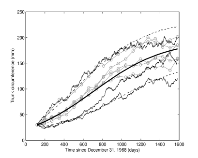
(a) $(M,n+1)=(5,20)$

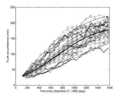
(b) $(M,n+1)=(30,20)$

Figure 1: Orange trees growth: simulated data (circles connected by straight lines) and fit of the SDMEM (12)-(13) using an order $K=2$ for the density expansion. In panel (a) is $(M,n+1)=(5,20)$ and in panel (b) is $(M,n+1)=(30,20)$. Each panel reports the empirical mean curve (smooth solid line), 95% empirical confidence curves (dashed lines) and example simulated trajectories.

There is a positive linear correlation ($r=0.42$, $p<0.001$) between the estimates of $\phi_{1}$ and $\phi_{3}$, see Figure 2 reporting also the least squares fit line. Similar relations were found when using different combinations of $M$ and $n$.

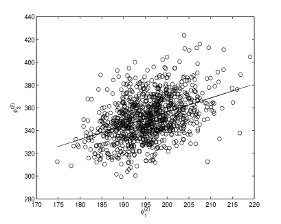
Figure 2: Orange trees growth: scatterplot of $\hat{\phi}_{3}^{(2)}$ vs $\hat{\phi}_{1}^{(2)}$ and least squares fit for $(M,n+1)=(30,20)$.

Histograms of the population parameter estimates $\hat{\phi}_{1}^{(2)}$, $\hat{\phi}_{3}^{(2)}$ and $\hat{\sigma}^{(2)}$ are given in Figure 3, with normal probability density functions fitted on top. The normal densities fit well to the histograms with estimated means (standard deviations) equal to 195.6 (6.6), 351.2 (19.2) and 0.080 (0.003) for $\hat{\phi}_{1}^{(2)}$, $\hat{\phi}_{3}^{(2)}$ and $\hat{\sigma}^{(2)}$, respectively.

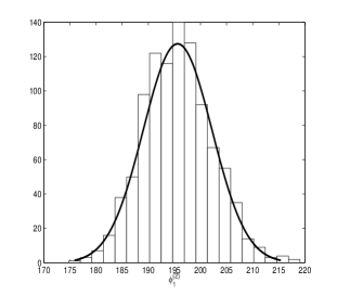
(a) $\hat{\phi}_{1}^{(2)}$

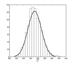
(b) $\hat{\phi}_{3}^{(2)}$

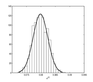
(c) $\hat{\sigma}^{(2)}$

Figure 3: Orange trees growth: histogram of population parameter estimates obtained using an order $K=2$ for the density expansion, and fits of normal probability density functions for $(M,n+1)=(30,20)$.

It is worthwhile to compare the methodology presented here, where a closed form expansion to the transition density is used, with a more straightforward approach, namely the approximation to the transition density based on the so-called “one-step” Euler-Maruyama approximation. Consider for ease of exposition a scalar SDE $dX_{t}=\mu(X_{t})dt+\sigma(X_{t})dW_{t}$ starting at $X_{0}=x_{0}$. The SDE can be approximated by $X_{t+\Delta}-X_{t}=\mu(X_{t})\Delta+\sigma(X_{t})\Delta^{1/2}\varepsilon_{t+\Delta}$ for $\Delta$ “small”, with $\{\varepsilon_{t+\Delta}\}$ a sequence of independent draws from the standard normal distribution. This leads to the following transition density approximation

$$p_{X}(x_{t+\Delta},\Delta\mid x_{t})\approx\varphi(x_{t+\Delta};x_{t}+\mu(x_{t})\Delta,\sigma^{2}(x_{t})\Delta)$$ (14)

where $\varphi(\cdot;m,v)$ is the pdf of the normal distribution with mean $m$ and variance $v$. The parameter estimates obtained using (14) instead of the closed-form approximation $p_{X}^{(K)}$ are given in Table 1 and are denoted EuM (standing for Euler-Maruyama). The value for $\Delta$ used in (14) is the time distance between the simulated data points. The comparisons between CFE and EuM for the same values of $M$ and $n$ have been performed using the same simulated datasets. The quality of the estimates obtained with the CFE method compared to the simple EuM approximation is considerable improved for data sampled at low frequency ($\Delta$ large), i.e. when $n=7$, which is a common situation in applications. For $(M=30,n=7)$ the 95% confidence intervals for the EuM method even fail to contain the true parameter values. The bad behavior of the EuM approximation when $\Delta$ is not small is well documented (e.g. Jensen and Poulsen (2002), Sørensen (2004)) and therefore our results are not surprising. Several experiments with different SDE models (not SDMEMs) have been conducted in Jensen and Poulsen (2002) where the conclusion is that although the CFE technique does require tedious algebraic calculations, they seem to be worth the effort.

5.2 Two-Dimensional Ornstein-Uhlenbeck Process

The OU process has found numerous applications in biology, physics, engineering and finance, see e.g. Picchini et al. (2008) and Ditlevsen and Lansky (2005) for applications in neuroscience, or Favetto and Samson (2010) for a two-dimensional OU model describing the tissue microvascularization in anti-cancer therapy.

Consider the following SDMEM of a two-dimensional OU process:

$$dX_{t}^{(1)i} = -\biggl{(}\beta_{11}b_{11}^{i}(X_{t}^{(1)i}-\alpha_{1})+\beta_{12}b_{12}^{i}(X_{t}^{(2)i}-\alpha_{2})\biggr{)}dt+\sigma_{1}dW_{t}^{(1)i},$$ (15)

$$dX_{t}^{(2)i} = -\biggl{(}\beta_{21}b_{21}^{i}(X_{t}^{(1)i}-\alpha_{1})+\beta_{22}b_{22}^{i}(X_{t}^{(2)i}-\alpha_{2})\biggr{)}dt+\sigma_{2}dW_{t}^{(2)i},$$ (16)

$$b^{i}_{ll^{{}^{\prime}}} \sim \Gamma(\nu_{ll^{\prime}},\nu_{ll^{\prime}}^{-1}),\qquad l,l^{{}^{\prime}}=1,2;\quad i=1,...,M$$ (17)

with initial values $X_{0}^{(k)i}=x_{0}^{(k)i},k=1,2$. Here $\Gamma(r,s)$ denotes the Gamma distribution with positive parameters $r$ and $s$ and probability density function

$$p_{\Gamma}(z)=\frac{1}{s^{r}\Gamma(r)}z^{r-1}e^{-z/s},\qquad z\geq 0,$$

with mean 1 when $s=r^{-1}$. The parameters $b_{ll^{\prime}}^{i}$, $\beta_{ll^{\prime}}$, $\sigma_{l}$ and $\nu_{ll^{\prime}}$ are strictly positive ($l,l^{\prime}=1,2$) whereas $\alpha_{1}$ and $\alpha_{2}$ are real. Let $*$ denote element-wise multiplication. Rewrite the system in matrix notation as

$$d\mathbf{X}_{t}^{i} = \boldsymbol{\beta}*\mathbf{b}^{i}(\boldsymbol{\alpha}-\mathbf{X}_{t}^{i})dt+\boldsymbol{\sigma}d\mathbf{W}_{t}^{i},\qquad\mathbf{X}_{0}^{i}=\mathbf{x}_{0}^{i},\quad i=1,...,M$$ (18)

where

$$\mathbf{X}_{t}^{i}=\left(\begin{array}[]{c}X_{t}^{(1)i}\\ X_{t}^{(2)i}\end{array}\right),\qquad\boldsymbol{\beta}=\left(\begin{array}[]{cc}\beta_{11}&\beta_{12}\\ \beta_{21}&\beta_{22}\end{array}\right),\qquad\mathbf{b}^{i}=\left(\begin{array}[]{cc}b_{11}^{i}&b_{12}^{i}\\ b_{21}^{i}&b_{22}^{i}\end{array}\right),$$

$$\boldsymbol{\alpha}=\left(\begin{array}[]{c}\alpha_{1}\\ \alpha_{2}\end{array}\right),\qquad\boldsymbol{\sigma}=\left(\begin{array}[]{cc}\sigma_{1}&0\\ 0&\sigma_{2}\end{array}\right),\qquad\mathbf{W}_{t}^{i}=\left(\begin{array}[]{c}W_{t}^{(1)i}\\ W_{t}^{(2)i}\end{array}\right),\qquad\mathbf{X}_{0}^{i}=\left(\begin{array}[]{c}X_{0}^{(1)i}\\ X_{0}^{(2)i}\end{array}\right).$$

The matrices $\boldsymbol{\beta}*\mathbf{b}^{i}$ and $\boldsymbol{\sigma}$ are assumed to have full rank. Assume the random effects are mutually independent and independent of $\mathbf{X}_{0}^{i}$ and $\mathbf{W}_{t}^{i}$. Because of (17) the random effects have mean one and therefore $\mathbb{E}(\boldsymbol{\beta}*\mathbf{b}^{i})=\boldsymbol{\beta}$ is the population mean. The set of parameters to be estimated in the external optimization step is $\boldsymbol{\theta}=(\alpha_{1},\alpha_{2},\beta_{11},\beta_{12},\beta_{21},\beta_{22},\sigma_{1},\sigma_{2})$ and $\boldsymbol{\Psi}=(\nu_{11},\nu_{12},\nu_{21},\nu_{22})$. However, during the internal optimization step it is necessary to estimate the $\mathbf{b}^{i}$’s also, that is $4M$ parameters. Thus, the total number of parameters in the overall estimation algorithm with internal and external steps is $12+4M$.

A stationary solution to (18) exists when the real parts of the eigenvalues of $\boldsymbol{\beta}*\mathbf{b}^{i}$ are strictly positive, i.e. $\boldsymbol{\beta}*\mathbf{b}^{i}$ has to be positive definite. The OU process is one of the only multivariate models with a known transition density other than multivariate models which reduce to the superposition of univariate processes. The transition density of model (18) for a given realization of the random effects is the bivariate Normal

$$p_{X}(\mathbf{x}_{j}^{i},\Delta_{j}^{i}|\mathbf{x}^{i}_{j-1},\mathbf{b}^{i},\boldsymbol{\theta})=(2\pi)^{-1}|\boldsymbol{\Omega}|^{-1/2}\exp(-(\mathbf{x}_{j}^{i}-\mathbf{m})^{T}\boldsymbol{\Omega}^{-1}(\mathbf{x}_{j}^{i}-\mathbf{m})/2)$$ (19)

with mean vector $\mathbf{m}=\boldsymbol{\alpha}+(\mathbf{x}^{i}_{j-1}-\boldsymbol{\alpha})\exp(-(\boldsymbol{\beta}*\mathbf{b}^{i})\Delta_{j}^{i})$ and covariance matrix $\boldsymbol{\Omega}=\boldsymbol{\lambda}-\exp(-(\boldsymbol{\beta}*\mathbf{b}^{i})\Delta_{j}^{i})\boldsymbol{\lambda}\exp(-(\boldsymbol{\beta}*\mathbf{b}^{i})^{T}\Delta_{j}^{i})$, where

$$\boldsymbol{\lambda}=\frac{1}{2\mathrm{tr}(\boldsymbol{\beta}*\mathbf{b}^{i})|\boldsymbol{\beta}*\mathbf{b}^{i}|}\bigl{(}|\boldsymbol{\beta}*\mathbf{b}^{i}|\boldsymbol{\sigma\sigma}^{T}+(\boldsymbol{\beta}*\mathbf{b}^{i}-\mathrm{tr}(\boldsymbol{\beta}*\mathbf{b}^{i})\mathbf{I})\boldsymbol{\sigma\sigma}^{T}(\boldsymbol{\beta}*\mathbf{b}^{i}-\mathrm{tr}(\boldsymbol{\beta}*\mathbf{b}^{i})\mathbf{I})^{T}\bigr{)}$$

is the $2\times 2$ matrix solution of the Lyapunov equation $(\boldsymbol{\beta}*\mathbf{b}^{i})\boldsymbol{\lambda}+\boldsymbol{\lambda}(\boldsymbol{\beta}*\mathbf{b}^{i})^{T}=\boldsymbol{\sigma\sigma}^{T}$ and $\mathbf{I}$ is the $2\times 2$ identity matrix (Gardiner (1985)). Here $|\mathbf{A}|$ denotes the determinant and $\mathrm{tr}(\mathbf{A})$ denotes the trace of a square matrix $\mathbf{A}$.

>From (18) we generated 1000 datasets of dimension $2(n+1)\times M$ and estimated the parameters using the proposed approximated method, thus obtaining 1000 sets of parameter estimates. A dataset consists of $2(n+1)$ observations at the equally spaced sampling times $\{0=t_{0}^{i}<t_{1}^{i}<\cdots<t_{n}^{i}=1\}$ for each of the $M$ experiments. The observations are obtained by linear interpolation from simulated trajectories using the Euler-Maruyama scheme with step size equal to $10^{-3}$ (Kloeden and Platen (1992)). We used the following set-up: $(X_{0}^{(1)i},X_{0}^{(2)i})$=(3, 3), $(\alpha_{1},\alpha_{2},\beta_{11},\beta_{12},\beta_{21},\beta_{22},\sigma_{1},\sigma_{2})$=(1, 1.5, 3, 2.5, 1.8, 2, 0.3, 0.5,), and $(\nu_{11},\nu_{12},\nu_{21},\nu_{22})$=(45, 100, 100, 25). An order $K=2$ approximation to the likelihood was used, see the Appendix for the coefficients of the transition density expansion. The estimates $(\boldsymbol{\hat{\theta}}^{(2)},\boldsymbol{\hat{\Psi}}^{(2)})$ are given in Table 2.

Table 2: Ornstein-Uhlenbeck model: Monte Carlo maximum likelihood estimates and 95% confidence intervals from 1000 simulations of model (18), using an order $K=2$ density expansion.

True parameter values					Estimates for $M=7$, $2(n+1)=40$
$\alpha_{1}$	$\alpha_{2}$	$\beta_{11}$	$\beta_{12}$		$\hat{\alpha}_{1}^{(2)}$	$\hat{\alpha}_{2}^{(2)}$	$\hat{\beta}_{11}^{(2)}$	$\hat{\beta}_{12}^{(2)}$
1	1.5	3	2.5	Mean [95% CI]	1.00 [0.59, 1.40]	1.50 [1.00, 1.97]	3.03 [2.50, 3.59]	2.50 [2.49, 2.51]
				Skewness	0.19	-0.32	0.21	3.17
				Kurtosis	5.27	5.73	3.29	59.60
$\beta_{21}$	$\beta_{22}$	$\sigma_{1}$	$\sigma_{2}$		$\hat{\beta}_{21}^{(2)}$	$\hat{\beta}_{22}^{(2)}$	$\hat{\sigma}_{1}^{(2)}$	$\hat{\sigma}_{2}^{(2)}$
1.8	2	0.3	0.5	Mean [95% CI]	1.61 [0.80, 2.14]	2.30 [1.56, 3.63]	0.307 [0.274, 0.339]	0.500 [0.494, 0.508]
				Skewness	-1.13	1.17	0.15	-1.10
				Kurtosis	5.45	4.77	3.05	46.62
$\nu_{11}$	$\nu_{12}$	$\nu_{21}$	$\nu_{22}$		$\hat{\nu}_{11}^{(2)}$	$\hat{\nu}_{12}^{(2)}$	$\hat{\nu}_{21}^{(2)}$	$\hat{\nu}_{22}^{(2)}$
45	100	100	25	Mean [95% CI]	104.79 [16.63, 171.62]	120.97 [5.90, 171.62]	105.97 [2.02, 171.62]	98.60 [4.92, 171.62]
				Skewness	-0.10	-0.72	-0.35	-0.17
				Kurtosis	1.26	2.13	1.74	1.25
True parameter values					Estimates for $M=20$, $2(n+1)=40$
$\alpha_{1}$	$\alpha_{2}$	$\beta_{11}$	$\beta_{12}$		$\hat{\alpha}_{1}^{(2)}$	$\hat{\alpha}_{2}^{(2)}$	$\hat{\beta}_{11}^{(2)}$	$\hat{\beta}_{12}^{(2)}$
1	1.5	3	2.5	Mean [95% CI]	1.00 [0.72, 1.27]	1.50 [1.19, 1.83]	3.01 [2.71, 3.32]	2.50 [2.50, 2.50]
				Skewness	-0.13	-0.17	0.14	0.01
				Kurtosis	7.01	6.84	3.32	34.66
$\beta_{21}$	$\beta_{22}$	$\sigma_{1}$	$\sigma_{2}$		$\hat{\beta}_{21}^{(2)}$	$\hat{\beta}_{22}^{(2)}$	$\hat{\sigma}_{1}^{(2)}$	$\hat{\sigma}_{2}^{(2)}$
1.8	2	0.3	0.5	Mean [95% CI]	1.71 [1.26, 2.03]	2.13 [1.72, 2.74]	0.307 [0.289, 0.327]	0.500 [0.495, 0.503]
				Skewness	-1.05	0.80	-0.01	1.69
				Kurtosis	5.23	3.96	3.00	41.16
$\nu_{11}$	$\nu_{12}$	$\nu_{21}$	$\nu_{22}$		$\hat{\nu}_{11}^{(2)}$	$\hat{\nu}_{12}^{(2)}$	$\hat{\nu}_{21}^{(2)}$	$\hat{\nu}_{22}^{(2)}$
45	100	100	25	Mean [95% CI]	83.35 [22.15, 171.62]	114.16 [18.18, 171.62]	105.00 [6.04, 171.62]	84.61 [7.36, 171.62]
				Skewness	0.66	-0.35	-0.26	0.24
				Kurtosis	1.83	1.86	1.84	1.26

The fit for $(M,2(n+1))=(20,40)$ is given in Figures 4(a)-4(b) for $X_{t}^{(1)i}$ and $X_{t}^{(2)i}$, respectively.

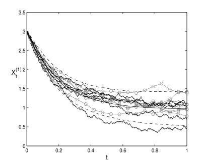
(a) $X_{t}^{(1)i}$

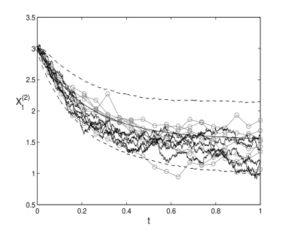
(b) $X_{t}^{(2)i}$

Figure 4: Ornstein-Uhlenbeck: simulated data (circles connected by straight lines), fit of $X_{t}^{(1)i}$ (panel (a)) and of $X_{t}^{(2)i}$ (panel (b)) from the SDMEM (18) for $(M,2(n+1))=(7,40)$. For each coordinate of the system the panels report the empirical mean curve of the SDMEM (smooth solid line), 95% empirical confidence curves (dashed lines) and five simulated trajectories.

Each figure reports the simulated data, the empirical mean of $5000$ simulated trajectories from (15)-(17), generated with the Euler-Maruyama scheme using a step size of length $10^{-3}$, the empirical 95% confidence bands of trajectory values as well as five example trajectories. For each simulated trajectory a realization of $b_{ll^{{}^{\prime}}}^{i}$ was produced by drawing from the $\Gamma(\nu_{ll}^{(2)},(\nu_{ll^{\prime}}^{(2)})^{-1})$ distribution using the estimates given in Table 2. The empirical correlations of the population parameter estimates is reported in Figure 5.

Figure 5: Ornstein-Uhlenbeck: scatterplot matrix of the estimates $(\hat{\alpha}_{1}^{(2)},\hat{\alpha}_{2}^{(2)},\hat{\beta}_{11}^{(2)},\hat{\beta}_{12}^{(2)},\hat{\beta}_{21}^{(2)},\hat{\beta}_{22}^{(2)},\hat{\sigma}_{1}^{(2)},\hat{\sigma}_{2}^{(2)})$ for $(M,2(n+1))=(20,40)$.

There is a strong negative correlation between the estimates of $\alpha_{1}$ and $\alpha_{2}$ ($r=-0.97$, $p<0.001$), which are the asymptotic means for $X_{t}^{(1)i}$ and $X_{t}^{(2)i}$. The sum $\hat{\alpha}_{1}^{(2)}+\hat{\alpha}_{2}^{(2)}$ results always almost exactly equal to 2.5 in each dataset ($\mathrm{mean}=2.50$, standard deviation = 0.04), so the sum is more precisely determined than each mean parameter. This occurs because there is a strong negative correlation between $X_{t}^{(1)i}$ and $X_{t}^{(2)i}$ equal to -0.898 in the stationary distribution in this numerical example. The individual mean parameters are unbiased but with standard deviations five times larger than the sum. There is a moderate negative correlation between $\beta_{21}$ and $\beta_{22}$ ($r=-0.53$, $p<0.001$).

The estimation method provides estimates for the $\mathbf{b}^{i}$’s also, given by the last values returned by the internal optimization step in the last round of the overall algorithm. An equivalent strategy is to plug $(\boldsymbol{\hat{\theta}}^{(2)},\boldsymbol{\hat{\Psi}}^{(2)})$ into (9) and then minimize $-f(\mathbf{b}^{i})$ w.r.t. $\mathbf{b}^{i}$ and obtain ${\boldsymbol{\hat{b}}^{i}}^{(2)}$. The estimation of the random effects is fast because we make use of the explicit Hessian, and for this example only 2-3 iterations of the internal step algorithm were necessary. We estimated the $\mathbf{b}^{i}$’s by plugging each of the 1000 sets of estimates into (9), thus obtaining the corresponding 1000 sets of estimates of $\mathbf{b}^{i}$. In Figure 6 boxplots of the estimates of the four random effects are reported for $M=7$, where estimates from different units have been pooled together.

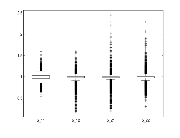
Figure 6: Ornstein-Uhlenbeck: boxplots of the random effects estimates ${\boldsymbol{\hat{b}}^{i}}^{(2)}$ for the SDMEM (18) for $(M,2(n+1))=(7,40)$.

For both $M=7$ and $M=20$ the estimates of the random effects have sample means equal to one, as it should be given the distributional hypothesis. The standard deviations of the true random effects are given by $1/\sqrt{\nu_{ll}}$ and thus equal 0.15, 0.1, 0.1 and 0.2 for $b_{11}^{i}$, $b_{12}^{i}$, $b_{21}^{i}$ and $b_{22}^{i}$, respectively. The empirical standard deviations of the estimated random effects for $M=7$ are 0.09, 0.09, 0.12 and 0.11, whereas for $M=20$ they are 0.09, 0.06, 0.08 and 0.09.

The parameters could be estimated by plugging the exact transition density (19) into (4) to form (9) and then maximize (10). However, the effort required for the estimation algorithm to converge is computationally costly, both using the analytic expression for the Hessian of $f$ in (10) or the one obtained using AD, since the Hessian has a huge expression when using the exact transition density. This problem is not present when using the density expansion because the expansion consists of polynomials of the parameters.

5.3 The square root SDMEM

The square root process is given by

$$dX_{t}=-\beta(X_{t}-\alpha)dt+\sigma\sqrt{X_{t}}dW_{t}.$$

This process is ergodic and its stationary distribution is the Gamma distribution with shape parameter $2\beta\alpha/\sigma^{2}$ and scale parameter $\sigma^{2}/(2\beta)$ provided that $\beta>0$, $\alpha>0$, $\sigma>0$, and $2\beta\alpha\geq\sigma^{2}$. The process has many applications: it is, for instance, used in mathematical finance to model short term interest rates where it is called the CIR process, see Cox et al. (1985). It is also a particular example of an integrate-and-fire model used to describe the evolution of the membrane potential in a neuron between emission of electrical impulses, see e.g. Ditlevsen and Lansky (2006) and references therein. In the neuronal literature it is called the Feller process, because William Feller proposed it as a model for population growth in 1951. Consider the SDMEM

$$dX_{t}^{i}=-\tilde{\beta}^{i}(X_{t}^{i}-\alpha-\alpha^{i})dt+\tilde{\sigma}^{i}\sqrt{X_{t}^{i}}dW_{t}^{i},\qquad i=1,...,M.$$ (20)

Assume $\alpha^{i}\sim\mathcal{B}(p_{\alpha},p_{\alpha})$, $\tilde{\sigma}^{i}\sim\mathcal{LN}(p_{\sigma_{1}},p_{\sigma_{2}}^{2})$ and $\tilde{\beta}^{i}\sim\mathcal{LN}(p_{\beta_{1}},p_{\beta_{2}}^{2})$. Here $\mathcal{LN}(\cdot,\cdot)$ denotes the (standard or 2-parameter) log-normal distribution and $\mathcal{B}(p_{\alpha},p_{\alpha})$ denotes the (generalized symmetric) Beta distribution on the interval $[a,b]$, with density function

$$p_{\mathcal{B}}(z)=\frac{1}{B(p_{\alpha},p_{\alpha})}\frac{(z-a)^{p_{\alpha}-1}(b-z)^{p_{\alpha}-1}}{(b-a)^{2p_{\alpha}-1}},\qquad p_{\alpha}>0,\quad a\leq z\leq b,$$

where $B(\cdot,\cdot)$ is the beta function and $a$ and $b$ are known constants. For ease of interpretation, assume the individual parameters $\tilde{\beta}^{i}$ and $\tilde{\sigma}^{i}$ to have unknown means $\beta$ and $\sigma$ respectively, e.g. assume $\tilde{\beta}^{i}=\beta+\beta^{i}$ and $\tilde{\sigma}^{i}=\sigma+\sigma^{i}$, $\beta^{i}$ and $\sigma^{i}$ being zero mean random quantities. This implies that $\beta$ and $\sigma$ do not need to be estimated directly: in fact the estimate for $\beta$ results determined via the moment relation $\beta=\exp(p_{\beta_{1}}+p_{\beta_{2}}^{2}/2)$ and can be calculated once estimates for $p_{\beta_{1}}$ and $p_{\beta_{2}}$ are available. Similarly, an estimate for $\sigma$ can be determined via $\sigma=\exp(p_{\sigma_{1}}+p_{\sigma_{2}}^{2}/2)$ by plugging in the estimates for $p_{\sigma_{1}}$ and $p_{\sigma_{2}}$.

The parameters to be estimated are $\theta=\alpha$, $\boldsymbol{\Psi}=(p_{\alpha},p_{\beta_{1}},p_{\beta_{2}},p_{\sigma_{1}},p_{\sigma_{2}})$ and $\mathbf{b}^{i}=(\alpha^{i},\tilde{\beta}^{i},\tilde{\sigma}^{i})$. To ensure that $X_{t}^{i}$ stays positive it is required that $2(\alpha+\alpha^{i})\tilde{\beta}^{i}/(\tilde{\sigma}^{i})^{2}\geq 1$. This condition must be checked in each iteration of the estimation algorithm. The means and variances of the population parameters added the random effects are

$$\mathbb{E}(\alpha+\alpha^{i})=\alpha+(a+b)/2 \mbox{Var}(\alpha+\alpha^{i})=(b-a)^{2}/(4(2p_{\alpha}+1)),$$ ;

$$\mathbb{E}(\tilde{\sigma}^{i})=\sigma=\exp(p_{\sigma_{1}}+p_{\sigma_{2}}^{2}/2) \mbox{Var}(\tilde{\sigma}^{i})=(\exp(p_{\sigma_{2}}^{2})-1)\exp(2p_{\sigma_{1}}+p_{\sigma_{2}}^{2}),$$ ;

$$\mathbb{E}(\tilde{\beta}^{i})=\beta=\exp(p_{\beta_{1}}+p_{\beta_{2}}^{2}/2) \mbox{Var}(\tilde{\beta}^{i})=(\exp(p_{\beta_{2}}^{2})-1)\exp(2p_{\beta_{1}}+p_{\beta_{2}}^{2}).$$ ;

For fixed values of the random effects, the asymptotic mean for the experimental unit $i$ is $\alpha+\alpha^{i}$. In most applications this value should be bounded within physical realistic values, and thus the Beta distribution was chosen for $\alpha^{i}$, since the support of the distribution of $\alpha+\alpha^{i}$ is then $[\alpha+a,\alpha+b]$. As in the previous examples, 1000 simulations were performed by generating equidistant observations in the time interval $[0,1]$ with the following setup: $(X_{0}^{i},\alpha,p_{\alpha},p_{\beta_{1}},p_{\beta_{2}},p_{\sigma_{1}},p_{\sigma_{2}})=(1,3,5,0,0.25,0.1,0.3)$ with fixed constants $[a,b]=[0.1,5]$. The coefficient of variations for $\alpha+\alpha^{i}$, $\tilde{\beta}^{i}$ and $\tilde{\sigma}^{i}$ are then 13.3%, 25.4% and 30.7%, respectively. The estimates obtained using an order $K=2$ density expansion are given in Table 3. A positive bias for $\hat{\alpha}^{(2)}$ is noticeable, however results are overall satisfactory, even using small sample sizes. Bias in estimates of drift parameters on finite observation intervals is a well known problem, and especially the speed parameter $\beta$ in mean reverting diffusion models is known to be biased and highly variable. In Tang and Chen (2009) the biases for $\beta$ in the OU and the square root model are calculated to be on the order of $T$, where $T$ is the length of the observation interval, and thus increasing $n$ does not improve the estimates unless the observation interval is also increased.

As described in the Ornstein-Uhlenbeck example, we have verified that the small sample distributions for the estimates of $\alpha^{i}$, $\tilde{\beta}^{i}$ and $\tilde{\sigma}^{i}$ have the expected characteristics: e.g. in the case $(M,n+1)=(5,7)$, by pooling together estimates from different units we have the following means (standard deviations) 2.61 (1.40), 0.95 (0.38) and 1.06 (0.29) for the estimates of $\alpha^{i}$, $\tilde{\beta}^{i}$ and $\tilde{\sigma}^{i}$, respectively. These values match well with the first moments of the true random effects $\mathbb{E}(\alpha^{i})=(0.1+5)/2=2.55$, $\mathbb{E}(\tilde{\beta}^{i})=1.03$ and $\mathbb{E}(\tilde{\sigma}^{i})=1.16$ and less well with the standard deviations $\mathrm{SD}_{\alpha^{i}}=0.74$, $\mathrm{SD}_{\tilde{\beta}^{i}}=0.26$ and $\mathrm{SD}_{\tilde{\sigma}^{i}}=0.35$. Average estimation time on a dataset of dimension $(M,n+1)=(10,20)$ was around 95 seconds and around 160 seconds when $(M,n+1)=(20,20)$, using a Matlab program on an Intel Core 2 Quad CPU (3 GHz).

Table 3: The square root model: Monte Carlo maximum likelihood estimates and 95% confidence intervals from 1000 simulations of model (20), using an order $K=2$ density expansion. Determined parameters are denoted with (*), i.e. true values for $\beta$ and $\sigma$ are determined according to the moment relations $\beta=\exp(p_{\beta_{1}}+p_{\beta_{2}}^{2}/2)$ and $\sigma=\exp(p_{\sigma_{1}}+p_{\sigma_{2}}^{2}/2)$. Estimates for determined parameters are calculated by plugging the estimates of $p_{\beta_{1,2}}$ and $p_{\sigma_{1,2}}$ obtained from each of the 1000 Monte Carlo simulations into the moment relations, then averaging over the 1000 determined values.

True parameter values					Estimates for $M=5$, $n+1=7$
$\alpha$	$\beta$ (*)	$\sigma$ (*)	$p_{\alpha}$		$\hat{\alpha}^{(2)}$	$\hat{\beta}^{(2)}$ (*)	$\hat{\sigma}^{(2)}$ (*)	$\hat{p}_{\alpha}^{(2)}$
3	1.03	1.16	5	Mean [95% CI]	4.06 [1,52, 9.85]	1.14 [0.51, 1.69]	1.13 [0.76, 1.60]	8.80 [0.94, 112.84]
				Skewness	1.23	0.49	0.60	4.37
				Kurtosis	4.46	3.20	4.72	22.47
$p_{\beta_{1}}$	$p_{\beta_{2}}$	$p_{\sigma_{1}}$	$p_{\sigma_{2}}$		$\hat{p}_{\beta_{1}}^{(2)}$	$\hat{p}_{\beta_{2}}^{(2)}$	$\hat{p}_{\sigma_{1}}^{(2)}$	$\hat{p}_{\sigma_{2}}^{(2)}$
0	0.25	0.1	0.3	Mean [95% CI]	-0.038 [-0.824, 0.177]	0.372 [0.001, 1.000]	0.082 [-0.278, 0.450]	0.173 [0.001, 0.561]
				Skewness	-2.92	0.79	-0.20	0.88
				Kurtosis	16.67	2.10	4.16	4.00
True parameter values					Estimates for $M=10$, $n+1=20$
$\alpha$	$\beta$ (*)	$\sigma$ (*)	$p_{\alpha}$		$\hat{\alpha}^{(2)}$	$\hat{\beta}^{(2)}$ (*)	$\hat{\sigma}^{(2)}$ (*)	$\hat{p}_{\alpha}^{(2)}$
3	1.03	1.16	5	Mean [95% CI]	4.43 [1.85, 9.63]	1.21 [0.44, 1.69]	1.15 [0.88, 1.48]	5.31 [0.99, 64.63]
				Skewness	1.01	-0.04	0.44	6.35
				Kurtosis	3.65	2.66	3.44	46.77
$p_{\beta_{1}}$	$p_{\beta_{2}}$	$p_{\sigma_{1}}$	$p_{\sigma_{2}}$		$\hat{p}_{\beta_{1}}^{(2)}$	$\hat{p}_{\beta_{2}}^{(2)}$	$\hat{p}_{\sigma_{1}}^{(2)}$	$\hat{p}_{\sigma_{2}}^{(2)}$
0	0.25	0.1	0.3	Mean [95% CI]	-0.045 [-0.953, 0.154]	0.487 [0.001, 1]	0.108 [-0.166, 0.376]	0.153 [0.001, 0.447]
				Skewness	-3.04	0.16	-0.03	0.71
				Kurtosis	14.65	1.40	3.29	2.84
True parameter values					Estimates for $M=20$, $n+1=20$
$\alpha$	$\beta$ (*)	$\sigma$ (*)	$p_{\alpha}$		$\hat{\alpha}^{(2)}$	$\hat{\beta}^{(2)}$ (*)	$\hat{\sigma}^{(2)}$ (*)	$\hat{p}_{\alpha}^{(2)}$
3	1.03	1.16	5	Mean [95% CI]	4.00 [2.35, 6.78]	1.21 [0.97, 1.68]	1.15 [0.98, 1.35]	2.33 [1.00, 5.00]
				Skewness	1.50	0.27	0.27	12.78
				Kurtosis	6.74	2.98	3.38	174.05
$p_{\beta_{1}}$	$p_{\beta_{2}}$	$p_{\sigma_{1}}$	$p_{\sigma_{2}}$		$\hat{p}_{\beta_{1}}^{(2)}$	$\hat{p}_{\beta_{2}}^{(2)}$	$\hat{p}_{\sigma_{1}}^{(2)}$	$\hat{p}_{\sigma_{2}}^{(2)}$
0	0.25	0.1	0.3	Mean [95% CI]	-0.011 [-0.069, 0.042]	0.498 [0.010, 1.000]	0.101 [-0.061, 0.256]	0.27 [0.13, 0.41]
				Skewness	-5.97	0.22	-0.02	-0.01
				Kurtosis	47.98	1.59	3.17	3.17

6 CONCLUSIONS

An estimation method for population models defined via SDEs, incorporating random effects, has been proposed and evaluated through simulations. SDE models with random effects have rarely been studied, as it is still non-trivial to estimate parameters in SDEs, even on single/individual trajectories, due to difficulties in deriving analytically the transition densities and the computational cost required to approximate the densities numerically. Approximation methods for transition densities is an important research topic, since a good approximation is necessary to carry out inferences based on the likelihood function, which guarantees well known optimal properties for the resulting estimators. Of the several approximate methods proposed in the last decades (see e.g. Sørensen (2004) and Hurn et al. (2007) for reviews) here we have considered the one suggested by Aït-Sahalia (2008) for the case of multidimensional SDEs, since it results in an accurate closed-form approximation for $p_{X}$ (Jensen and Poulsen (2002)).

In this work SDEs with multiple random effects have been studied, moving a step forward with respect to the results presented in Picchini et al. (2010), where Gaussian quadrature was used to solve the integrals for a single random effect. The latter approach results unfeasible when there are several random effects because the dimension of the integral grows. In fact, it may be difficult to numerically evaluate the integral in (3) and (7) when $\mathbf{b}^{i}\in B\subseteq\mathbb{R}^{q}$, with $q$ much larger than 2, and efficient numerical algorithms are needed. As noted by Booth et al. (2001), if e.g. $q=20$ one cannot count on standard statistical software to maximize the likelihood, and numerical integration quadrature is only an option if the dimension of the integral is low, whereas it quickly becomes unreliable when the dimension grows. Some references are the review paper by Cools (2002), Krommer and Ueberhuber (1998) and references therein, or one of the several monographs on Monte Carlo methods (e.g. Ripley (2006)). In the mixed-effects framework the amount of literature devoted to the evaluation of $q$-dimensional integrals is large, see e.g. Davidian and Giltinan (2003), Pinheiro and Bates (1995), McCulloch and Searle (2001) and Pinheiro and Chao (2006). We decided to use the Laplace approximation because using a symbolic calculus software it is relatively easy to obtain the Hessian matrix necessary for the calculations, which results useful also to speed up the optimization algorithm.

Computing derivatives of long expressions can be a tedious and error prone task even with the help of a software for symbolic calculus. In those cases we reverted to software for automatic differentiation (AD, e.g. Griewank (2000)). Although the present work does not necessarily rely on AD tools, it is worthwhile to spend a few words to describe roughly what AD is, since it is relatively unknown in the statistical community even if it has already been applied in the mixed-effects field (Skaug (2002); Skaug and Fournier (2006)). AD should not be confused with symbolic calculus since it does not produce analytic expressions for the derivatives/Hessians of a given function, i.e. it does not produce expressions meant to be understood by the human eye. Instead, given a program computing some function $h(u)$, the application of AD on $h(u)$ produces another program implementing the calculations necessary to compute gradients, Hessians etc. of $h(u)$ exactly (to machine precision); furthermore, AD can differentiate programs including e.g. for loops or if-else statements, which are outside the scope of symbolic differentiation. See http://www.autodiff.org for a list of AD software tools. However, the possibility of easily deriving gradients and Hessians using AD comes at a price. The code produced by AD to compute the derivatives of $h(u)$ may result so long and complex that it might affect negatively the performance of the overall estimation procedure, when invoked into an optimization procedure. Thus, we suggest to use analytic expressions whenever possible. However, at the very least, an AD program can still be useful to check whether analytically obtained results are correct or not. Modellers and practitioners might consider the software AD Model Builder (ADMB Project (2009)), providing a framework integrating AD, model building and data fitting tools, which comes with its own module for mixed-effects modelling.

This work has a number of limitations, mostly due to the difficulty in carrying out the closed-form approximation to the likelihood for multidimensional SDEs ($d\geq 2$). It is even more difficult when the diffusion is not reducible, although mathematical methods to treat this case are available (Aït-Sahalia (2008)). Another limitation is that measurement error is not modelled, which is a problem if this noise source is not negligible relatively to the system noise. The R PSM package is capable of modelling measurement error and uses the Extended Kalman Filter (EKF) to estimate SDMEMs (Klim et al. (2009)). EKF provides approximations for the individual likelihoods which are exact only for linear SDEs. The closed-form expansion considered in the present work can instead provide an approximation as good as desired to the individual likelihood (8) by increasing the order $K$ of the expansion, though it can be a tedious task. Like in the present paper, PSM considers a Laplace approximation to multidimensional integrals, but Hessians are obtained using an approximation to the second order derivatives (first order conditional estimation, FOCE); in our work Hessians are obtained exactly (to machine precision) using automatic differentiation. Unfortunately, the structural differences between our method and PSM make a rigorous comparison between the two methods impossible, even simply in terms of computational times, since PSM requires the specification of a measurement error factor and thus both the observations and the number of parameters considered in the estimation are different. Finally, PSM assumes multivariate normally distributed effects only, whereas in our method this restriction is not necessary.

We believe the class of SDMEMs to be useful in applications, especially in those areas where mixed-effects theory is used routinely, e.g. in biomedical and pharmacokinetic/pharmacodynamic studies. From a theoretical point of view SDMEMs are necessary when analyzing repeated measurements data if both the variability between experiments to obtain more precise estimates of population characteristics, as well as stochasticity in the individual dynamics should be taken into account.

Appendix A REDUCIBILITY AND DENSITY EXPANSION COEFFICIENTS

A.1 Reducible diffusions

The following is a necessary and sufficient condition for the reducibility of a multivariate diffusion process (Aït-Sahalia (2008)):

Proposition 1.

The diffusion $\mathbf{X}$ is reducible if and only if

$$\sum_{q=1}^{d}\frac{\partial\sigma_{ik}(\mathbf{x})}{\partial x^{(q)}}\sigma_{qj}(\mathbf{x})=\sum_{q=1}^{d}\frac{\partial\sigma_{ij}(\mathbf{x})}{\partial x^{(q)}}\sigma_{qk}(\mathbf{x})$$

for each $\mathbf{x}$ in $E$ and triplet $(i,j,k)=1,...,d$. If $\boldsymbol{\sigma}$ is nonsingular, then the condition is

$$\frac{\partial\{\boldsymbol{\sigma}^{-1}\}_{ij}(\mathbf{x})}{\partial x^{(k)}}=\frac{\partial\{\boldsymbol{\sigma}^{-1}\}_{ik}(\mathbf{x})}{\partial x^{(j)}}$$

where $\{\boldsymbol{\sigma}^{-1}\}_{ij}(\mathbf{x})$ is the $(i,j)$-th element of $\boldsymbol{\sigma}^{-1}(\mathbf{x})$.

A.2 General expressions for the density expansion coefficients

Here are reported the explicit expressions for the coefficients of the log-density expansion (6) as given in Aït-Sahalia (2008). The use of a symbolic algebra program is advised for the practical calculation of the coefficients. For two given $d$-dimensional values $\mathbf{y}$ and $\mathbf{y}_{0}$ of the process $\mathbf{Y}_{t}=\boldsymbol{\gamma}(\mathbf{X}_{t})$ the coefficients of the log-density expansion are given by

$$C_{Y}^{(-1)}(\mathbf{y}|\mathbf{y}_{0}) = -\frac{1}{2}\sum_{h=1}^{d}(y^{(h)}-y_{0}^{(h)})^{2},$$

$$C_{Y}^{(0)}(\mathbf{y}|\mathbf{y}_{0}) = \sum_{h=1}^{d}(y^{(h)}-y_{0}^{(h)})\int_{0}^{1}\mu_{Y}^{(h)}(\mathbf{y}_{0}+u(\mathbf{y}-\mathbf{y}_{0}))du$$

$$C_{Y}^{(k)}(\mathbf{y}|\mathbf{y}_{0}) = k\int_{0}^{1}G_{Y}^{(k)}(\mathbf{y}_{0}+u(\mathbf{y}-\mathbf{y}_{0})|\mathbf{y}_{0})u^{k-1}du.$$

for $k\geq 1$. The functions $G_{Y}^{(k)}$ are given by

$$G_{Y}^{(1)}(\mathbf{y}|\mathbf{y}_{0})=-\sum_{h=1}^{d}\frac{\partial\mu_{Y^{(h)}}(\mathbf{y})}{\partial y^{(h)}}-\sum_{h=1}^{d}\mu_{Y^{(h)}}(\mathbf{y})\frac{\partial C^{(0)}_{Y}(\mathbf{y}|\mathbf{y}_{0})}{\partial y^{(h)}}+\frac{1}{2}\sum_{h=1}^{d}\biggl{\{}\frac{\partial^{2}C^{(0)}_{Y}(\mathbf{y}|\mathbf{y}_{0})}{\partial{y^{(h)}}^{2}}+\biggl{(}\frac{\partial C^{(0)}_{Y}(\mathbf{y}|\mathbf{y}_{0})}{\partial y^{(h)}}\biggr{)}^{2}\biggr{\}}$$

and for $k\geq 2$

$$G_{Y}^{(k)}(\mathbf{y}|\mathbf{y}_{0}) = -\sum_{h=1}^{d}\mu_{Y^{(h)}}(\mathbf{y})\frac{\partial C_{Y}^{(k-1)}(\mathbf{y}|\mathbf{y}_{0})}{\partial y^{(h)}}+\frac{1}{2}\sum_{h=1}^{d}\frac{\partial^{2}C_{Y}^{(k-1)}(\mathbf{y}|\mathbf{y}_{0})}{\partial{y^{(h)}}^{2}}$$

$$+\frac{1}{2}\sum_{h=1}^{d}\sum_{h^{{}^{\prime}}=0}^{k-1}\binom{k-1}{h^{{}^{\prime}}}\frac{\partial C_{Y}^{(h^{{}^{\prime}})}(\mathbf{y}|\mathbf{y}_{0})}{\partial y^{(h)}}\frac{\partial C_{Y}^{(k-1-h^{{}^{\prime}})}(\mathbf{y}|\mathbf{y}_{0})}{\partial y^{(h)}}.$$

A.3 Coefficients of the orange trees growth SDMEM

In model (12)-(13) is $Y_{t}^{i}=\gamma(X_{t}^{i})=2\sqrt{X_{t}^{i}}/\sigma$ so $\mu_{Y}(Y_{t}^{i})=Y_{t}^{i}(\phi_{1}+\phi_{1}^{i}-\sigma^{2}{Y_{t}^{i}}^{2}/4)/(2(\phi_{3}+\phi_{3}^{i})(\phi_{1}+\phi_{1}^{i}))-1/(2Y_{t}^{i})$, and for given values $y_{j}^{i}$ and $y_{j-1}^{i}$ of $Y_{t}^{i}$, we have

$$C_{Y}^{(-1)}(y^{i}_{j}|y_{j-1}^{i}) = -\frac{1}{2}(y^{i}_{j}-y_{j-1}^{i})^{2}$$

$$C_{Y}^{(0)}(y_{j}^{i}|y_{j-1}^{i}) = -\frac{\sigma^{2}({y_{j}^{i}}^{4}-{y_{j-1}^{i}}^{4})}{32(\phi_{3}+\phi_{3}^{i})(\phi_{1}+\phi_{1}^{i})}+\frac{{(y_{j}^{i}}^{2}-{y_{j-1}^{i}}^{2})}{4(\phi_{3}+\phi_{3}^{i})}-\frac{1}{2}\log\left(\frac{y_{j}^{i}}{y_{j-1}^{i}}\right)$$

$$C_{Y}^{(1)}(y_{j}^{i}|y_{j-1}^{i}) = -\frac{\sigma^{4}\left({y_{j}^{i}}^{6}+{y_{j}^{i}}^{5}y_{j-1}^{i}+{y_{j}^{i}}^{4}{y_{j-1}^{i}}^{2}+(y_{j}^{i}y_{j-1}^{i})^{3}+{y_{j}^{i}}^{2}{y_{j-1}^{i}}^{4}+y_{j}^{i}{y_{j-1}^{i}}^{5}+{y_{j-1}^{i}}^{6}\right)}{896(\phi_{3}+\phi_{3}^{i})^{2}(\phi_{1}+\phi_{1}^{i})^{2}}$$

$$+\frac{\sigma^{2}(10(\phi_{3}+\phi_{3}^{i})({y_{j}^{i}}^{2}+y_{j}^{i}y_{j-1}^{i}+{y_{j-1}^{i}}^{2})+3({y_{j}^{i}}^{5}+{y_{j}^{i}}^{2}y_{j-1}^{i}+{y_{j-1}^{i}}^{3}))}{240(\phi_{3}+\phi_{3}^{i})^{2}(\phi_{1}+\phi_{1}^{i})}$$

$$-\frac{9(\phi_{3}+\phi_{3}^{i})^{2}+y_{j}^{i}y_{j-1}^{i}({y_{j}^{i}}^{2}+y_{j}^{i}y_{j-1}^{i}+{y_{j-1}^{i}}^{2})}{24y_{j}^{i}y_{j-1}^{i}(\phi_{3}+\phi_{3}^{i})^{2}}$$

$$C_{Y}^{(2)}(y_{j}^{i}|y_{j-1}^{i}) = -\frac{\sigma^{4}(5({y_{j}^{i}}^{4}+{y_{j-1}^{i}}^{4})+8y_{j}^{i}y_{j-1}^{i}({y_{j}^{i}}^{2}+{y_{j-1}^{i}}^{2})+9{y_{j}^{i}}^{2}{y_{j-1}^{i}}^{2})}{896(\phi_{3}+\phi_{3}^{i})^{2}(\phi_{1}+\phi_{1}^{i})^{2}}$$

$$+\frac{\sigma^{2}\left(9({y_{j}^{i}}^{2}+{y_{j-1}^{i}}^{2})+12y_{j}^{i}y_{j-1}^{i}+10(\phi_{3}+\phi_{3}^{i})\right)}{240(\phi_{3}+\phi_{3}^{i})^{2}(\phi_{1}+\phi_{1}^{i})}-\frac{({y_{j}^{i}}^{2}{y_{j-1}^{i}}^{2}+9(\phi_{3}+\phi_{3}^{i})^{2})}{24{y_{j}^{i}}^{2}{y_{j-1}^{i}}^{2}(\phi_{3}+\phi_{3}^{i})^{2}}$$

and

$$p_{X}^{(2)}(x_{j}^{i},\Delta_{j}^{i}|x_{j-1}^{i}) = \frac{1}{\sqrt{2\pi\sigma^{2}\Delta_{j}^{i}x_{j}^{i}}}\exp\biggl{(}-\frac{2\biggl{(}\sqrt{x_{j}^{i}}-\sqrt{x_{j-1}^{i}}\biggr{)}^{2}}{\sigma^{2}\Delta_{j}^{i}}+\tilde{C}^{(0)}(x_{j}^{i}|x_{j-1}^{i})$$

$$+ \tilde{C}^{(1)}(x_{j}^{i}|x_{j-1}^{i})\Delta_{j}^{i}+\frac{{\Delta_{j}^{i}}^{2}}{2}\tilde{C}^{(2)}(x_{j}^{i}|x_{j-1}^{i})\biggl{)}$$

where $\tilde{C}^{(k)}(x_{j}^{i}|x_{j-1}^{i})=C_{Y}^{(k)}\left(\frac{2\sqrt{x_{j}^{i}}}{\sigma}\Big{|}\frac{2\sqrt{x_{j-1}^{i}}}{\sigma}\right),\,k=0,1,2$.

A.4 Coefficients of the two-dimensional OU SDMEM

The process (15)-(16) is reducible and $\boldsymbol{\gamma}(\mathbf{x}^{i})=\boldsymbol{\sigma}^{-1}\mathbf{x}^{i}=(x^{(1)i}/\sigma_{1},x^{(2)i}/\sigma_{2})^{T}$, so

$$d\mathbf{Y}_{t}^{i}=\bigl{(}\boldsymbol{\sigma}^{-1}(\boldsymbol{\beta}*\mathbf{b}^{i})\boldsymbol{\alpha}-\boldsymbol{\sigma}^{-1}(\boldsymbol{\beta}*\mathbf{b}^{i})\boldsymbol{\sigma}\mathbf{Y}_{t}^{i}\bigr{)}dt+d\mathbf{W}_{t}^{i}:=\boldsymbol{\kappa}^{i}(\boldsymbol{\eta}-\mathbf{Y}_{t}^{i})dt+d\mathbf{W}_{t}^{i}$$

where $\boldsymbol{\eta}=\boldsymbol{\sigma}^{-1}\boldsymbol{\alpha}=(\eta_{1},\eta_{2})^{T}$ and $\boldsymbol{\kappa}^{i}=\boldsymbol{\sigma}^{-1}(\boldsymbol{\beta}*\mathbf{b}^{i})\boldsymbol{\sigma}=\{\kappa^{i}_{q,q^{{}^{\prime}}}\}_{q,q^{{}^{\prime}}=1,2}$. If $\mathbf{y}^{i}_{j}=(y^{(1)i}_{j},y^{(2)i}_{j})^{T}$ and $\mathbf{y}_{j-1}^{i}=(y^{(1)i}_{j-1},y^{(2)i}_{j-1})^{T}$ are two values from $\mathbf{Y}_{t}^{i}$, the coefficients of the order $K=2$ density expansion (6) for model (15)-(16) are given by:

$$C_{Y}^{(-1)}(\mathbf{y}^{i}_{j}|\mathbf{y}_{j-1}^{i}) = -\frac{1}{2}(y^{(1)i}_{j}-y_{j-1}^{(1)i})^{2}-\frac{1}{2}(y^{(2)i}_{j}-y_{j-1}^{(2)i})^{2},$$

$$C_{Y}^{(0)}(\mathbf{y}^{i}_{j}|\mathbf{y}_{j-1}^{i}) = -\frac{1}{2}(y^{(1)i}_{j}-y_{j-1}^{(1)i})((y^{(1)i}_{j}+y_{j-1}^{(1)i}-2\eta_{1})\kappa_{11}^{i}+(y^{(2)i}_{j}+y_{j-1}^{(2)i}-2\eta_{2})\kappa_{12}^{i})$$

$$-\frac{1}{2}(y^{(2)i}_{j}-y_{j-1}^{(2)i})((y^{(1)i}_{j}+y_{j-1}^{(1)i}-2\eta_{1})\kappa_{21}^{i}+(y^{(2)i}_{j}+y_{j-1}^{(2)i}-2\eta_{2})\kappa_{22}^{i}),$$

$$C_{Y}^{(1)}(\mathbf{y}^{i}_{j}|\mathbf{y}_{j-1}^{i}) = \frac{1}{2}(\kappa_{11}^{i}-((y_{j-1}^{(1)i}-\eta_{1})\kappa_{11}^{i}+(y_{j-1}^{(2)i}-\eta_{2})\kappa_{12}^{i})^{2})$$

$$+\frac{1}{2}(\kappa_{22}^{i}-((y_{j-1}^{(1)i}-\eta_{1})\kappa_{21}^{i}+(y_{j-1}^{(2)i}-\eta_{2})\kappa_{22}^{i})^{2})$$

$$-\frac{1}{2}(y^{(1)i}_{j}-y_{j-1}^{(1)i})((y_{j-1}^{(1)i}-\eta_{1})({\kappa_{11}^{i}}^{2}+{\kappa_{21}^{i}}^{2})+(y_{j-1}^{(2)i}-\eta_{2})(\kappa_{11}^{i}\kappa_{12}^{i}+\kappa_{21}^{i}\kappa_{22}^{i}))$$

$$+\frac{1}{24}(y^{(1)i}_{j}-y_{j-1}^{(1)i})^{2}(-4{\kappa_{11}^{i}}^{2}+{\kappa_{12}^{i}}^{2}-2\kappa_{12}^{i}\kappa_{21}^{i}-3{\kappa_{21}^{i}}^{2})$$

$$-\frac{1}{2}(y^{(2)i}_{j}-y_{j-1}^{(2)i})((y_{j-1}^{(1)i}-\eta_{1})(\kappa_{11}^{i}\kappa_{12}^{i}\kappa_{21}^{i}\kappa_{22}^{i})$$

$$+(y_{j-1}^{(2)i}-\eta_{2})((\kappa_{12}^{i})^{2}+(\kappa_{22}^{i})^{2}))$$

$$+\frac{1}{24}(y^{(2)i}_{j}-y_{j-1}^{(2)i})^{2}(-4(\kappa_{22}^{i})^{2}+(\kappa_{21}^{i})^{2}-2\kappa_{12}^{i}\kappa_{21}^{i}-3(\kappa_{12}^{i})^{2})$$

$$-\frac{1}{3}(y^{(1)i}_{j}-y_{j-1}^{(1)i})(y^{(2)i}_{j}-y_{j-1}^{(2)i})(\kappa_{11}^{i}\kappa_{12}^{i}+\kappa_{21}^{i}\kappa_{22}^{i}),$$

$$C_{Y}^{(2)}(\mathbf{y}^{i}_{j}|\mathbf{y}_{j-1}^{i}) = -\frac{1}{12}(2{\kappa_{11}^{i}}^{2}+2{\kappa_{22}^{i}}^{2}+(\kappa_{12}^{i}+\kappa_{21}^{i})^{2})$$

$$+\frac{1}{6}(y^{(1)i}_{j}-y_{j-1}^{(1)i})(\kappa_{12}^{i}-\kappa_{21}^{i})((y_{j-1}^{(1)i}-\eta_{1})(\kappa_{11}^{i}\kappa_{12}^{i}+\kappa_{21}^{i}\kappa_{22}^{i})+(y_{j-1}^{(2)i}-\eta_{2})({\kappa_{12}^{i}}^{2}+{\kappa_{22}^{i}}^{2}))$$

$$+\frac{1}{12}(y^{(1)i}_{j}-y_{j-1}^{(1)i})^{2}(\kappa_{12}^{i}-\kappa_{21}^{i})(\kappa_{11}^{i}\kappa_{12}^{i}+\kappa_{21}^{i}\kappa_{22}^{i})$$

$$+\frac{1}{12}(y^{(2)i}_{j}-y_{j-1}^{(2)i})^{2}(\kappa_{21}^{i}-\kappa_{12}^{i})(\kappa_{11}^{i}\kappa_{12}^{i}+\kappa_{21}^{i}\kappa_{22}^{i})$$

$$+\frac{1}{6}(y^{(2)i}_{j}-y_{j-1}^{(2)i})(\kappa_{21}^{i}-\kappa_{12}^{i})((y_{j-1}^{(1)i}-\eta_{1})({\kappa_{11}^{i}}^{2}+{\kappa_{21}^{i}}^{2})$$

$$+(y_{j-1}^{(2)i}-\eta_{2})(\kappa_{11}^{i}\kappa_{12}^{i}+\kappa_{21}^{i}\kappa_{22}^{i}))$$

$$+\frac{1}{12}(y^{(1)i}_{j}-y_{j-1}^{(1)i})(y^{(2)i}_{j}-y_{j-1}^{(2)i})(\kappa_{12}^{i}-\kappa_{21}^{i})({\kappa_{22}^{i}}^{2}+{\kappa_{12}^{i}}^{2}-{\kappa_{11}^{i}}^{2}+{\kappa_{21}^{i}}^{2}).$$

A.5 Coefficients of the square root SDMEM

For model (20) we have

$$Y_{t}^{i}=\frac{2\sqrt{X_{t}^{i}}}{\tilde{\sigma}^{i}}$$

and

$$\mu_{Y}(Y_{t}^{i})=\frac{2q+1}{2Y_{t}^{i}}-\frac{\tilde{\beta}^{i}Y_{t}^{i}}{2},$$

where $q=2\tilde{\beta}^{i}(\alpha+\alpha^{i})/(\tilde{\sigma}^{i})^{2}-1$. For given values $y_{j-1}^{i}$ and $y^{i}_{j}$ of $Y_{t}^{i}$ the coefficients of the order $K=2$ density expansion are:

$$C_{Y}^{(-1)}(y^{i}_{j}|y_{j-1}^{i}) = -\frac{1}{2}(y^{i}_{j}-y_{j-1}^{i})^{2},$$

$$C_{Y}^{(0)}(y^{i}_{j}|y_{j-1}^{i}) = \log\biggl{(}\frac{y^{i}_{j}}{y_{j-1}^{i}}\biggr{)}\biggl{(}q+\frac{1}{2}\biggr{)}-\frac{1}{4}\tilde{\beta}^{i}({y^{i}_{j}}^{2}-{y_{j-1}^{i}}^{2}),$$

$$C_{Y}^{(1)}(y^{i}_{j}|y_{j-1}^{i}) = -\frac{1}{24y_{j-1}^{i}y^{i}_{j}}\bigl{[}-12\tilde{\beta}^{i}y^{i}_{j}y_{j-1}^{i}(q+1)+(\tilde{\beta}^{i})^{2}({y^{i}_{j}}^{3}y_{j-1}+(y^{i}_{j}y_{j-1}^{i})^{2}$$

$$+ y^{i}_{j}{y_{j-1}^{i}}^{3})+12q^{2}-3\bigr{]},$$

$$C_{Y}^{(2)}(y^{i}_{j}|y_{j-1}^{i}) = =-\frac{1}{24(y^{i}_{j}y_{j-1}^{i})^{2}}\bigl{[}(\tilde{\beta}^{i})^{2}(y^{i}_{j}y_{j-1}^{i})^{2}+12q^{2}-3\bigr{]}.$$

References

- ADMB Project (2009) ADMB Project, 2009. AD Model Builder: automatic differentiation model builder. Developed by David Fournier and freely available from admb-project.org.
- Aït-Sahalia (2008) Aït-Sahalia, Y., 2008. Closed-form likelihood expansion for multivariate diffusions. Ann. Stat. 36 (2), 906–937.
- Allen (2007) Allen, E., 2007. Modeling with Itô Stochastic Differential Equations. Springer.
- Bischof et al. (2005) Bischof, C., Bücker, M., Vehreschild, A., 2005. ADiMat. RWTH Aachen University, Germany, available at http://www.sc.rwth-aachen.de/adimat/.
- Booth et al. (2001) Booth, J., Hobert, J., Jank, W., 2001. A survey of Monte Carlo algorithms for maximizing the likelihood of a two-stage hierarchical model. Statistical Modelling 1, 333–349.
- Coleman and Li (1996) Coleman, T., Li, Y., 1996. An interior, trust region approach for nonlinear minimization subject to bounds. SIAM Journal on Optimization 6, 418–445.
- Cools (2002) Cools, R., 2002. Advances in multidimensional integration. Journal of Computational and Applied Mathematics 149, 1–12.
- Cox et al. (1985) Cox, J., Ingersoll, J., Ross, S., 1985. A theory of the term structure of interest rate. Econometrica 53, 385–407.
- Davidian and Giltinan (2003) Davidian, M., Giltinan, D., 2003. Nonlinear models for repeated measurements: an overview and update. Journal of Agricultural, Biological, and Environmental Statistics 8, 387–419.
- D’Errico (2006) D’Errico, J., 2006. fminsearchbnd. Bound constrained optimization using fminsearch, http://www.mathworks.com/matlabcentral/fileexchange/8277-fminsearchbnd.
- Ditlevsen and De Gaetano (2005) Ditlevsen, S., De Gaetano, A., 2005. Mixed effects in stochastic differential equations models. REVSTAT - Statistical Journal 3 (2), 137–153.
- Ditlevsen and Lansky (2005) Ditlevsen, S., Lansky, P., 2005. Estimation of the input parameters in the Ornstein-Uhlenbeck neuronal model. Physical Review E 71, 011907.
- Ditlevsen and Lansky (2006) Ditlevsen, S., Lansky, P., 2006. Estimation of the input parameters in the Feller neuronal model. Phys. Rev. E 73, Art. No. 061910.
- Donnet et al. (2010) Donnet, S., Foulley, J., Samson, A., 2010. Bayesian analysis of growth curves using mixed models defined by stochastic differential equations. Biometrics 66 (3), 733–741.
- Donnet and Samson (2008) Donnet, S., Samson, A., 2008. Parametric inference for mixed models defined by stochastic differential equations. ESAIM: Probability & Statistics 12, 196–218.
- Favetto and Samson (2010) Favetto, B., Samson, A., 2010. Parameter estimation for a bidimensional partially observed Ornstein-Uhlenbeck process with biological application. Scandinavian Journal of Statistics 37, 200–220.
- Filipe et al. (2010) Filipe, P., Braumann, C., Roquete, C., 2010. Multiphasic individual growth models in random environments. Methodology and Computing in Applied Probability, 1–8. 10.1007/s11009-010-9172-0.
- Gardiner (1985) Gardiner, C., 1985. Handbook of Stochastic Methods for Physics, Chemistry and the Natural Sciences. Springer.
- Griewank (2000) Griewank, A., 2000. Evaluating Derivatives: Principles and Techniques of Algorithmic Differentiation. SIAM Philadelphia, PA.
- Hurn et al. (2007) Hurn, A., Jeisman, J., Lindsay, K., 2007. Seeing the wood for the trees: A critical evaluation of methods to estimate the parameters of stochastic differential equations. Journal of Financial Econometrics 5 (3), 390–455.
- Jensen and Poulsen (2002) Jensen, B., Poulsen, R., 2002. Transition densities of diffusion processes: numerical comparison of approximation techniques. Journal of Derivatives 9, 1–15.
- Joe (2008) Joe, H., 2008. Accuracy of Laplace approximation for discrete response mixed models. Computational Statistics & Data Analyis 52 (12), 5066–5074.
- Klim et al. (2009) Klim, S., Mortensen, S. B., Kristensen, N. R., Overgaard, R. V., Madsen, H., 2009. Population stochastic modelling (PSM) – An R package for mixed-effects models based on stochastic differential equations. Computer Methods and Programs in Biomedicine 94, 279–289.
- Kloeden and Platen (1992) Kloeden, P., Platen, E., 1992. Numerical Solution of Stochastic Differential Equations. Springer.
- Ko and Davidian (2000) Ko, H., Davidian, M., 2000. Correcting for measurement error in individual-level covariates in nonlinear mixed effects models. Biometrics 56 (2), 368–375.
- Krommer and Ueberhuber (1998) Krommer, A., Ueberhuber, C., 1998. Computational Integration. Society for Industrial and Applied Mathematics.
- Lindstrom and Bates (1990) Lindstrom, M., Bates, D., 1990. Nonlinear mixed-effects models for repeated measures data. Biometrics 46, 673–687.
- McCulloch and Searle (2001) McCulloch, C., Searle, S., 2001. Generalized, Linear and Mixed Models. Wiley Series in Probability and Statistics. John Wiley & Sons, Inc.
- Øksendal (2007) Øksendal, B., 2007. Stochastic Differential Equations: An Introduction With Applications, sixth Edition. Springer.
- Overgaard et al. (2005) Overgaard, R., Jonsson, N., Tornøe, C., Madsen, H., 2005. Non-linear mixed-effects models with stochastic differential equations: implementation of an estimation algorithm. Journal of Pharmacokinetics and Pharmacodynamics 32, 85–107.
- Picchini et al. (2010) Picchini, U., De Gaetano, A., Ditlevsen, S., 2010. Stochastic differential mixed-effects models. Scandinavian Journal of Statistics 37 (1), 67–90.
- Picchini et al. (2008) Picchini, U., Ditlevsen, S., De Gaetano, A., Lansky, P., 2008. Parameters of the diffusion leaky integrate-and-fire neuronal model for a slowly fluctuating signal. Neural Computation 20 (11), 2696–2714.
- Pinheiro and Bates (1995) Pinheiro, J., Bates, D., 1995. Approximations of the log-likelihood function in the nonlinear mixed-effects model. Journal of Computational and Graphical Statistics 4 (1), 12–35.
- Pinheiro and Bates (2002) Pinheiro, J., Bates, D., 2002. Mixed-effects models in S and S-PLUS. Springer-Verlag, NY.
- Pinheiro et al. (2007) Pinheiro, J., Bates, D., DebRoy, S., Sarkar, D., the R Development Core Team, 2007. The nlme Package. R Foundation for Statistical Computing, http://www.R-project.org/.
- Pinheiro and Chao (2006) Pinheiro, J., Chao, E., 2006. Efficient Laplacian and adaptive Gaussian quadrature algorithms for multilevel generalized linear mixed models. Journal of Computational and Graphical Statistics 15 (1), 58–81.
- Ripley (2006) Ripley, B., 2006. Stochastic Simulation. Wiley-Interscience.
- Shun and McCullagh (1995) Shun, Z., McCullagh, P., 1995. Laplace approximation of high dimensional integrals. Journal of the Royal Statistical Society B 57 (4), 749–760.
- Skaug (2002) Skaug, H., 2002. Automatic differentiation to facilitate maximum likelihood estimation in nonlinear random effects models. Journal of Computational and Graphical Statistics 11 (2), 458–470.
- Skaug and Fournier (2006) Skaug, H., Fournier, D., 2006. Automatic approximation of the marginal likelihood in non-Gaussian hierarchical models. Computational Statistics & Data Analysis 51, 699–709.
- Sørensen (2004) Sørensen, H., 2004. Parametric inference for diffusion processes observed at discrete points in time: a survey. International Statistical Review 72 (3), 337–354.
- Strathe et al. (2009) Strathe, A., Sørensen, H., Danfær, A., 2009. A new mathematical model for combining growth and energy intake in animals: The case of the growing pig. Journal of Theoretical Biology 261 (2), 165 – 175.
- Tang and Chen (2009) Tang, C., Chen, S., 2009. Parameter estimation and bias correction for diffusion processes. Journal of Econometrics 149 (1), 65–81.
- Tornøe et al. (2005) Tornøe, C., Overgaard, R., Agersø, H., Nielsen, H., Madsen, H., Jonsson, E. N., 2005. Stochastic differential equations in NONMEM: implementation, application, and comparison with ordinary differential equations. Pharmaceutical Research 22 (8), 1247–1258.