Pooling Design and Bias Correction in DNA Library Screening

Abstract

We study the group test for DNA library screening based on probabilistic approach. Group test is a method of detecting a few positive items from among a large number of items, and has wide range of applications. In DNA library screening, positive item corresponds to the clone having a specified DNA segment, and it is necessary to identify and isolate the positive clones for compiling the libraries. In the group test, a group of items, called pool, is assayed in a lump in order to save the cost of testing, and positive items are detected based on the observation from each pool. It is known that the design of grouping, that is, pooling design is important to achieve accurate detection. In the probabilistic approach, positive clones are picked up based on the posterior probability. Naive methods of computing the posterior, however, involves exponentially many sums, and thus we need a device. Loopy belief propagation (loopy BP) algorithm is one of popular methods to obtain approximate posterior probability efficiently. There are some works investigating the relation between the accuracy of the loopy BP and the pooling design. Based on these works, we develop pooling design with small estimation bias of posterior probability, and we show that the balanced incomplete block design (BIBD) has nice property for our purpose. Some numerical experiments show that the bias correction under the BIBD is useful to improve the estimation accuracy.

*4mm Nagoya UniversityFurocho, Chikusaku, Nagoya 464-8603, Japan kanamori@is.nagoya-u.ac.jp Nagoya UniversityFurocho, Chikusaku, Nagoya 464-8603, Japan uehara@jim.math.cm.is.nagoya-u.ac.jp Nagoya UniversityFurocho, Chikusaku, Nagoya 464-8603, Japan jimbo@is.nagoya-u.ac.jp

1 Introduction

We study the group test based on a probabilistic approach. Group test is a method of detecting positive items out of a set of a large number of items, and has wide range of applications such as blood test or DNA library screening.

In the context of DNA library screening, our purpose is to identify clones having a specified DNA fragment from among a collection of DNA segments. Each DNA segment is called clones. The clone with a specified segment is referred to as positive clone, otherwise negative clone. For large libraries, it is impractical to screen each clone individually, instead a group of clones, called pool, is assayed in a lump. This is said to be group test or pooling experiment. When a pool gives positive result, the pool contains at least one positive clone, and otherwise all clones are negative. A number of pools are prepared, and outcomes from all pools are assembled to identify positive clones.

There are mainly two categories of group test; one is adaptive, and the other is non-adaptive. In adaptive strategy, the pool is sequentially prepared and the test is conducted based on the information of previous outcomes. By repeating the test procedure, we can narrow down the set of positive clones. In non-adaptive testing, we prepare all pools to be tested before conducting the group test. The positive clones are detected based on the outcome of each pool. That is, the grouping of clones does not depend on the result of previous testing. When the group test for each pool is performed by distinct experimenters, non-adaptive method may not be time-consuming compared to adaptive one. In this article, we focus on non-adaptive testing.

In group testing, we have two kind of detecting procedure; one is combinatorial and the other is probabilistic. In combinatorial group testing, the main issue is to construct the design of grouping or pooling design to reduce the number of testing without missing the positive clones. Combinatorial group testing has been studied by many authors (Du and Hwang, 1999; Ngo and Du, 2000; Wu et al., 2004). In combinatorial approach, it is often assumed that the maximum number of positive clones is known and that there is no observation errors or noisy measurements. On the other hand, in probabilistic approach the prior probability for the state of clones is assumed, and posterior probability such that each clone is positive is computed based on the observation of each pool (Knill et al., 1996; Bruno et al., 1995; Mézard and Toninelli, 2007; Uehara and Jimbo, 2009). The main issue is to develop efficient algorithm to compute the posterior probability, since using naive Bayes formula is computationally demanding. Knill et al. (1996) and Uehara and Jimbo (2009) have proposed a probabilistic algorithm. Knill et al. (1996) have used the Markov Chain Monte Carlo (MCMC) method to obtain the marginal posterior probability, and Uehara and Jimbo (2009) have exploited the loopy belief propagation (BP) algorithm (Pearl, 1988; MacKay, 1999) to compute approximate probability.

Non-adaptive group test with probabilistic approach will be one of the most practical methods to detect positive clones from among large DNA library. Even in probabilistic approach, the pooling design is significant to achieve highly accurate estimation of posterior probability. In loopy BP algorithm for the low density parity check (LDPC) coding (MacKay, 1999; Richardson et al., 2001), it has been revealed that the coding design is closely related to the decoding error of the transmitted code. Likewise, the pooling design with some nice property will provide accurate estimator of the posterior probability as experimentally shown by Uehara and Jimbo (2009). In coding theory, Ikeda et al. (2004a) have analyzed the relation between the coding design and the bias of the estimated posterior probability. We apply their result to improve the accuracy of the group testing.

The outline of the paper is as follows. In Section 2 probabilistic description of group testing for DNA library screening is presented. In Section 3 we introduce loopy belief propagation algorithm, and in Section 4 we show the bias the estimated posterior probability according to Ikeda et al. (2004a). In Section 5, we construct a pooling design resulting in a small bias. Numerical experiments are presented in Section 6. Section 7 is devoted to concluding remarks.

2 Preliminaries of DNA library screening

On DNA library screening, our purpose is to identify the positive clones out of a large DNA library. Let $X_{i}$ be the random variable which stands for the label of the clone $i$ for $i=1,\ldots,n$, that is, $X_{i}=1$ for positive and $X_{i}=0$ for negative. The labels of all clones are denoted as the vector $X=(X_{1},\ldots,X_{n})$. We assume that the random variables $X_{i},\,i=1,\ldots,n$ are independent. The probability such that $X=x\in\{0,1\}^{n}$ for $x=(x_{1},\ldots,x_{n})$ is denoted by $p(x)$ or $p(X=x)$. Then, the probability $p(x)$ is represented by the factorization of marginal probabilities, that is

$$p(x)=p_{1}(x_{1})\times\cdots\times p_{n}(x_{n}).$$

Since the marginal distribution $p_{i}(x_{i})$ over $\{0,1\}$ is written as the form of exponential model $p_{i}(x_{i})\propto\exp\{h_{i}x_{i}\}$, the joint probability $p(x)$ is given as

$$p(x)=\exp\{h^{\top}x-\psi_{0}(h)\},\quad x\in\{0,1\}^{n}$$

with $h=(h_{1},\ldots,h_{n})\in\mathbb{R}^{n}$, where $\psi_{0}(h)$ is the normalization factor called the cumulant generating function.

In the group test a number of clones are set in a pool and the experiment is conducted to detect if a positive close is included in the pool. Here the pool is identified by a subset of $\{1,\ldots,n\}$, and the clone $i$ is included in the pool $r$ if and only if $i\in r$ holds. For the pool $r\subset\{1,\ldots,n\}$, let $Z_{r}$ be the random variable defined by

$$Z_{r}=\begin{cases}1&{}^{\exists}i\in r,\ X_{i}=1,\\ 0&\text{otherwise}.\end{cases}$$ (1)

Hence if $Z_{r}=1$, there is a positive clone in the pool $r$. Note that $Z_{r}$ is also represented as

$$Z_{r}=\max_{i\in r}X_{i}=1-\prod_{i\in r}(1-X_{i}).$$

In practice, $Z_{r}$ is not directly observed. The observation of the pool $r$ is usually represented by four levels such that

$$S_{r}=\begin{cases}0&\text{if the pool $r$ is negative},\\ 1&\text{if the pool $r$ is weak positive},\\ 2&\text{if the pool $r$ is medium positive},\\ 3&\text{if the pool $r$ is strong positive}.\end{cases}$$

The response of the experiment is measured by using a fluorescence sign, and it is experimentally-confirmed that the conditional probability of $S_{r}$ given $X_{i},(i\in r)$ only depends on $Z_{r}$, not the number of $i\in r$ such that $X_{i}=1$. We assume that the conditional probability of $S_{r}$ given $Z_{r}$ is the same for all pools. Then, the conditional probability of $S_{r}=s_{r}$ given $Z_{r}=z_{r}$ is denoted as $p(S_{r}=s_{r}|Z_{r}=z_{r})$ or $p(s_{r}|z_{r})$. In practice $p(S_{r}=0|Z_{r}=0)$ and $p(S_{r}=3|Z_{r}=1)$ will take larger value than others. In the group test usually we prepare a number of pools. Let $\mathcal{G}=\{r_{1},\ldots,r_{m}\}$ be the set of pools used in the group test. Then for each pool $r\in\mathcal{G}$ the observation $s_{r}\in\{0,1,2,3\}$ is obtained. An example of a pooling design is shown in Figure 1.

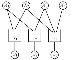
Figure 1: An example of a pooling design. $\mathcal{G}$ is given as $\{\{1,2\},\,\{1,3\},\,\{2,3,4\}\}$.

The problem considered in the paper is to infer the label of clones based on the observation from each pool. More precisely, we want to pick up only positive clones out of all clones. As a probabilistic approach, the method of maximum a posteriori (MAP) estimate is useful to detect the positive clones. Let $S=(S_{1},\ldots,S_{m})$ be the random variable for the observation from all pools, and

$$p(X=x|S=s)=p(x|s)$$

be the posterior probability of $X=x=(x_{1},\ldots,x_{n})$ given $S=s=(s_{1},\ldots,s_{m})$, where $m$ is the number of pools. The label pattern $x\in\{0,1\}^{n}$ maximizing the posterior $p(x|s)$ will provide the set of clones which are likely to be positive.

We represent the posterior $p(x|s)$ by $p(x)$ and $p(s|x)$. Using the Bayes formula, we can represent the posterior probability $p(x|s)$ as

$$p(x|s)\propto p(s|x)p(x).$$

For the distinct pools $r,r^{\prime}\in\mathcal{G}$, the observations $s_{r}$ and $s_{r^{\prime}}$ are conditionally independent for given $x$. Hence the probability $p(s|x)$ is decomposed into the conditional probabilities of $r\in\mathcal{G}$, and then we have

$$p(s|x)=\prod_{r\in\mathcal{G}}p(s_{r}|x).$$

For each observation $s\in\{0,1,2,3\}$, the conditional probability $p(S_{r}=s|x)$ is written as

$$p(S_{r}=s|x)\propto\exp\{c(s,x)\}$$

as the function of $s$, where $c(s,x)$ is a real-valued function. When we compute the posterior probability of $p(x|s)$, the observations $s_{r},r\in\mathcal{G}$ are regarded as constants, and thus $c(s_{r},x)$ is written as $c_{r}(x)$ as the function of the label pattern $x\in\{0,1\}^{n}$. Note that $c_{r}(x)$ depends only on $z_{r}$ which is a realized value of $Z_{r}$ defined in (1). Then, the posterior probability $p(x|s)$ is given as

$$p(x|s)\propto\exp\big{\{}h^{\top}x+\sum_{r\in\mathcal{G}}c_{r}(x)\big{\}}.$$ (2)

Suppose that the parameter $h$ and the functions $c_{r}(x),\,r\in\mathcal{G}$ are known or these are estimated with satisfactory accuracy.

In general the maximization of $p(x|s)$ in (2) over $x\in\{0,1\}^{n}$ is computationally hard unless the set of pools $\mathcal{G}$ has some special property (Pearl, 1988; Cowell et al., 2007). Thus, we take another approach. The marginal probability of $x_{i}$ for $p(x|s)$ is denoted as $p_{i}(x_{i}|s)$, that is

$$p_{i}(x_{i}|s)=\sum_{x^{\prime}\in\{0,1\}^{n}\,:\,x^{\prime}_{i}=x_{i}}p(x^{\prime}|s)$$ (3)

We think that the clones having large marginal posterior $p_{i}(X_{i}=1|s)$ will be positive. Using a threshold for the marginal posterior, we will be able to detect the set of positive clones. As an example Table 1 shows exact marginal posterior probabilities $p_{i}(X_{i}=1|s)$. The pooling design in Figure 1 and the observation probability $p(S_{r}=s|x)$ shown in Table 5 are used, and the marginal probability $p(X_{i}=1)$ is set to $0.1$ for all clones. We see that the marginal posterior will be useful to detect the positive clones.

Table 1: An example of marginal posterior probabilities. The pooling design in Figure 1 and the observation probability $p(S_{r}=s|x)$ shown in Table 5 are used, and the marginal probability $p(X_{i}=1)$ is set to $0.1$ for all clones.

$(s_{1},s_{2},s_{3})\in\{0,1,2,3\}^{3}$	$p_{1}(X_{1}=1|s)$	$p_{2}(X_{2}=1|s)$	$p_{3}(X_{3}=1|s)$	$p_{4}(X_{4}=1|s)$
$(3,0,0)$	0.043	0.047	0.001	0.011
$(2,2,0)$	0.853	0.019	0.019	0.009
$(0,1,3)$	0.020	0.016	0.760	0.180
$(0,0,3)$	0.001	0.027	0.027	0.429

The computation of the marginal posterior is still hard, since there are exponentially many summands in (3). Despite this, we can compute an approximate posterior probability by applying so-called loopy belief propagation (loopy BP) algorithm. The details of loopy BP is briefly introduced in Section 3.

3 Loopy Belief Propagation for Computation of Marginal Probability

Loopy belief propagation is a method of computing an approximate marginal probability, which is very useful in stochastic reasoning (Pearl, 1988; Cowell et al., 2007). Let $q(x)$ be a joint probability of high dimensional binary variable $x=(x_{1},\ldots,x_{n})\in\{0,1\}^{n}$. In the group test $q(x)$ corresponds to the posterior probability $p(x|s)$. The computation of the marginal $q_{i}(x_{i})$ involves exponentially many sums. To reduce the computational cost, we approximate the joint probability $q(x)$ by a tractable one. Suppose that $q(x)$ is represented by the form of (2), that is,

$$q(x)\propto\exp\big{\{}h^{\top}x+\sum_{r\in\mathcal{G}}c_{r}(x)\big{\}}$$ (4)

and we use the model

$$\bar{q}(x;\theta)\propto\exp\big{\{}h^{\top}x+\theta^{\top}x\}$$ (5)

to approximate $q(x)$, where $\theta=(\theta_{1},\ldots,\theta_{n})^{\top}\in\mathbb{R}^{n}$ is an $n$ dimensional column vector. The parameter $\theta$ is determined such that the function $\theta^{\top}x$ is close to $\sum_{r\in\mathcal{G}}c_{r}(x)$ up to additive constant. Then, the marginal probability of $q(x)$ will be approximately given by

$$\bar{q}_{i}(x_{i};\theta)\propto\exp\big{\{}h_{i}x_{i}+\theta_{i}x_{i}\big{\}},\quad i=1,\ldots,n.$$

As a result, we can obtain an approximate value of the marginal probability for $q(x)$. The loopy BP algorithm provides an efficient method of computing the parameter $\theta$. Suppose that $\theta$ is decomposed into the sum of parameters $\xi_{r}\in\mathbb{R}^{n},\,r\in\mathcal{G}$, that is,

$$\theta=\sum_{r\in\mathcal{G}}\xi_{r}.$$

We suppose that the function $c_{r}(x)$ is approximated by $\xi_{r}^{\top}x$ for each pool $r\in\mathcal{G}$. When the parameters $\xi_{r},\,r\in\mathcal{G}$ are obtained in mid-flow of the algorithm, we show how to update these parameters. Let $\zeta_{r}$ be defined as

$$\zeta_{r}=\sum_{s\in\mathcal{G}}\xi_{s}-\xi_{r}=\theta-\xi_{r}.$$

When the function $c_{r}(x)$ is approximated by $\xi_{r}^{\top}x$, the probability $q(x)$ is also approximated by $\exp\{h^{\top}x+\zeta_{r}^{\top}x+c_{r}(x)\}$. We seek the parameter $\bar{\xi}_{r}$ such that $\exp\{h^{\top}x+\zeta_{r}^{\top}x+\bar{\xi}_{r}^{\top}x\}$ approximates $\exp\{h^{\top}x+\zeta_{r}^{\top}x+c_{r}(x)\}$ up to the normalization constant. The Kullback-Leibler divergence

$${\rm KL}(p,q)=\sum_{x\in\{0,1\}^{n}}p(x)\log\frac{p(x)}{q(x)}$$

is used as the discrepancy measure between two probabilities $p$ and $q$ over $\{0,1\}^{n}$. We consider the following optimization problem:

$$\min_{\xi_{r}\in\mathbb{R}^{n}}{\rm KL}(p,q)$$

$$\phantom{\min}\text{subject to}\ \ p(x)\propto\exp\{h^{\top}x+\zeta_{r}^{\top}x+c_{r}(x)\},\quad q(x)\propto\exp\{h^{\top}x+\zeta_{r}^{\top}x+\xi_{r}^{\top}x\}.$$

By some calculation, we see that the above problem is represented as the following form:

$$\begin{array}[]{l}\displaystyle\max_{\xi_{r}\in\mathbb{R}^{n}}\sum_{x\in\{0,1\}^{n}}\exp\{h^{\top}x+\zeta_{r}^{\top}x+c_{r}(x)\}\vspace*{1mm}\displaystyle\cdot\bigg{\{}\xi_{r}^{\top}x-\sum_{i=1}^{n}\log(1+\exp\{h_{i}+\zeta_{ri}+\xi_{ri}\})\bigg{\}}.\end{array}$$ (7)

There are $2^{|r|}$ summands in the function to be optimized, where $|r|$ denotes the number of elements in the set $r$. When the size of the pool $r$ is not large, the objective function in the optimization problem above is tractable. The parameter $\xi_{r}$ is updated to $\bar{\xi}_{r}$ which is the optimal solution of (7). In the same way, the parameters $\xi_{r},r\in\mathcal{G}$ and the sum $\theta=\sum_{r\in\mathcal{G}}\xi_{r}$ are updated sequentially. The convergent point of $\theta$ is the output of the algorithm, and we obtain the approximated marginal probability $\bar{q}_{i}(x_{i};\theta),i=1,\ldots,n$. The loopy BP algorithm is very useful in practice, though the convergence property of the algorithm is not theoretically guaranteed under general condition.

In the literature of DNA library screening, the function $c_{r}(x)$ depends on the value of $z_{r}=\max_{i\in r}x_{i}$, and thus we define

$$c_{r}(x)=\begin{cases}c_{r1}&z_{r}=1,\\ c_{r0}&z_{r}=0.\end{cases}$$

Then, the objective function of (7) has a simple form, and the updated parameter $\bar{\xi}_{r}$ in the loopy BP algorithm is explicitly obtained. See Uehara and Jimbo (2009) for details.

4 Bias of Loopy Belief Propagation

According to Ikeda et al. (2004a) we show the bias introduced by the loopy BP algorithm in the general setup. For each pool $r\in\mathcal{G}$, let $c_{r}(x)$ be any real-valued function depending only on $x_{i},i\in r$, and $q(x)$ be a probability on $\{0,1\}^{n}$ defined as the form of (4). Let $q_{i}(x_{i})$ be the marginal probability of $q(x)$. We use the statistical model (5) to approximate the joint probability $q(x)$. Let $\bar{q}(x;\theta_{0})\propto\exp\{h^{\top}x+\theta_{0}^{\top}x\}$ be the convergent joint probability computed by the loopy BP algorithm applied to $q(x)$. Usually the estimated marginal $\bar{q}_{i}(x_{i};\theta_{0})$ is not equal to the true marginal probability $q_{i}(x_{i})$, and the difference $q_{i}(x_{i})-\bar{q}_{i}(x_{i};\theta_{0})$ is said to be bias. Ikeda et al. (2004a) have analyzed the bias of the loopy BP algorithm, and obtained the asymptotic formula such that

$$q_{i}(1)-\bar{q}_{i}(1;\theta_{0})~{}=~{}\frac{1}{2}\sum_{\begin{subarray}{c}r,s\in\mathcal{G}\\ r\neq s\end{subarray}}B_{rsi}\ +\text{(higher order terms)},$$ (8)

where $B_{rsi}$ is related to a geometrical curvature of statistical model $\bar{q}(x;\theta)$.

To show the definition of $B_{rsi}$, we need to define the matrices $g_{ij},g_{ir},\widetilde{g}_{ir}$ and the third order tensor $T$. Let $\bar{x}_{i}$ and $\bar{c}_{r}$ be the expectation of $x_{i}$ and $c_{r}(x)$ under $\bar{q}(x;\theta_{0})$, that is

$$\bar{x}_{i}=\sum_{x_{i}}x_{i}\bar{q}_{i}(x_{i};\theta_{0}),\qquad\bar{c}_{r}=\sum_{x}c_{r}(x)\bar{q}(x;\theta_{0}).$$

Note that the expectation $\bar{x}_{i}$ is equal to $q_{i}(1;\theta_{0})$, since $x_{i}$ is the binary variable. The matrix $g_{ij},i,j=1,\ldots,n$ is the Fisher information matrix of the model $\bar{q}(x;\theta)$ at $\theta=\theta_{0}$,

$$g_{ij}=\sum_{x_{i},x_{j}}(x_{i}-\bar{x}_{i})(x_{j}-\bar{x}_{j})\bar{q}(x;\theta_{0})=\delta_{ij}\sum_{x_{i}}(x_{i}-\bar{x}_{i})^{2}\bar{q}_{i}(x_{i};\theta_{0})=\delta_{ij}\bar{x}_{i}(1-\bar{x}_{i}),$$

where $\delta_{ij}$ is the Kronecker’s delta function such that $\delta_{ij}=1$ for $i=j$ and otherwise $\delta_{ij}=0$. Likewise the matrix $g_{ir}$ for $i=1,\ldots,n,\ r\in\mathcal{G}$ is defined by

$$g_{ir}=\sum_{x}(x_{i}-\bar{x}_{i})(c_{r}(x)-\bar{c}_{r})\bar{q}(x;\theta_{0}),$$

and let $\widetilde{g}_{ir}$ be $\widetilde{g}_{ir}=g_{ir}/g_{ii}$. Moreover let the third tensor $T$ be

$$T_{ijk} =\sum_{x}(x_{i}-\bar{x}_{i})(x_{j}-\bar{x}_{j})(x_{k}-\bar{x}_{k})\bar{q}(x;\theta_{0}),\quad i,j,k=1,\ldots,n,$$

$$T_{ijr} =\sum_{x}(x_{i}-\bar{x}_{i})(x_{j}-\bar{x}_{j})(c_{r}(x)-\bar{c}_{r})\bar{q}(x;\theta_{0}),\quad i,j=1,\ldots,n,\ r\in\mathcal{G},$$

$$T_{irs} =\sum_{x}(x_{i}-\bar{x}_{i})(c_{r}(x)-\bar{c}_{r})(c_{s}(x)-\bar{c}_{s})\bar{q}(x;\theta_{0}),\quad i=1,\ldots,n,\ r,s\in\mathcal{G}.$$

Then $B_{irs}$ is defined as

$$B_{rsi}=-T_{irs}-\sum_{j,k=1}^{n}T_{ijk}\widetilde{g}_{jr}\widetilde{g}_{ks}+\sum_{j=1}^{n}(T_{ijr}\widetilde{g}_{js}+T_{ijs}\widetilde{g}_{jr}),\quad i=1,\ldots,n,\ \ r,s\in\mathcal{G}.$$ (9)

Once we obtain the approximate joint probability $\bar{q}(x;\theta_{0})$, we can compute $B_{rsi}$ without knowing the target probability $q(x)$. Thus, according to (8) the bias is corrected by adding $\sum_{r\neq s}B_{rsi}/2$ to $\bar{q}_{i}(1;\theta_{0})$.

5 Relation between Pooling Design and Bias of Loopy BP Algorithm

We show some properties of $B_{rsi}$ defined in (9). Let $c_{r}(x)$ be the function on $\{0,1\}^{n}$ depending only on $x_{i},i\in r$, then $c_{r}(x)$ is represented as the form of

$$c_{r}(x)~{}=~{}h_{r}+\sum_{\ell}b_{r\ell}\prod_{i\in r}(x_{i}-a_{r\ell i}),\quad h_{r},\ b_{r\ell}\in\mathbb{R},\ a_{r\ell i}\in[0,1].$$ (10)

This fact is shown below. Let $r=\{i_{1},\ldots,i_{|r|}\}\subset\{1,\ldots,n\}$, and $\bar{x}$ be $\bar{x}=(\bar{x}_{1},\ldots,\bar{x}_{|r|})\in\{0,1\}^{|r|}$, then we define $c_{r}(x)$ by

$$c_{r}(x)=\sum_{\bar{x}\in\{0,1\}^{|r|}}\ b_{\bar{x}}\prod_{j=1}^{|r|}\big{(}1-(x_{i_{j}}-\bar{x}_{j})^{2}\big{)}=\sum_{\bar{x}\in\{0,1\}^{|r|}}\bigg{[}b_{\bar{x}}\prod_{k=1}^{|r|}(2\bar{x}_{k}-1)\bigg{]}\prod_{j=1}^{|r|}\big{(}x_{i_{j}}-(1-\bar{x}_{j})\big{)}.$$ (11)

The function $c_{r}(x)$ has the form of (10), and the variable $x\in\{0,1\}^{n}$ satisfying $x_{i_{j}}=\bar{x}_{j}$ for $j=1,\ldots,|r|$ is mapped to $b_{\bar{x}}\in\mathbb{R}$. By varying $b_{\bar{x}}$ any function over $\{0,1\}^{n}$ can be represented by the form above. Though the parameter $a_{r\ell i}$ in (10) can be restricted to the binary set $\{0,1\}$, we allow the mild condition $a_{r\ell i}\in[0,1]$ for convenience.

Example 1.

For the group test

$$c_{r}(x)=\rho_{r}\cdot\max_{i\in r}x_{i}=\rho_{r}\{1-(-1)^{|r|}\prod_{i\in r}(x_{i}-1)\}$$

is used. For the low density parity check (LDPC) codes the function

$$c_{r}(x)=\rho_{r}\cdot\prod_{i\in r}(1-2x_{i})=\rho_{r}(-2)^{|r|}\prod_{i\in r}(x_{i}-1/2)$$

is exploited. In the above, the coefficient $\rho_{r}$ determines the intensity contributed from the pool $r\in\mathcal{G}$.

First, we show the condition that the bias vanishes.

Theorem 1.

Let $c_{r}$ be real-valued function over $\{0,1\}^{n}$ depending only on the variables $x_{i},\,i\in r$. Let $r,s$ be distinct subsets of $\{1,\ldots,n\}$. Then, for any functions $c_{r}(x),\,c_{s}(x)$ and any $i=1,\ldots,n$, $B_{rsi}$ vanishes if $|r\cap s|\leq 1$.

Theorem 1 is a direct conclusion of Theorem 7 in Ikeda et al. (2004a). The proof is deferred to appendix A to show the explicit form of $B_{rsi}$. Let the packing design be the family of sets $\mathcal{G}$ satisfying $|r\cap s|\leq 1$ for any $r,s\in\mathcal{G}$, then Theorem 1 denotes that for the packing design the dominant bias term of loopy BP algorithm vanishes. The packing design is used in the design of group test (Uehara and Jimbo, 2009) and also in the LDPC code (MacKay, 1999). It is numerically shown that the accuracy of approximate probability is superior to other designs with $|r\cap s|\geq 2$. In coding theory, lots of designs of low density parity check (LDPC) code have been intensively studied, and the packing design is known as good error-correcting code (Ikeda et al., 2004a; MacKay, 1999). In Theorem 1 these results are extended to any function $c_{r},r\in\mathcal{G}$.

We consider the bias term $B_{rsi}$ for $|r\cap s|\geq 2$.

Theorem 2.

Let $c_{r}$ and $c_{s}$ be functions with the form of (10), and suppose that there exists a constant $C$ such that the coefficients $b_{r\ell},b_{s\ell}$ satisfy

$$\sum_{\ell,\ell^{\prime}}\big{|}b_{r\ell}b_{s\ell^{\prime}}\big{|}\leq C.$$

Let $\bar{x}_{i}$ be the expectation of $x_{i}$ under the probability $\bar{q}(x;\theta_{0})\propto\exp\{h^{\top}x+\theta_{0}^{\top}x\}$ and $\delta$ be a real number satisfying

$$0<|\bar{x}_{i}-a_{r\ell i}|\leq\delta<1,\quad 0<|\bar{x}_{i}-a_{s\ell i}|\leq\delta<1,$$

for any $i,\ell,r,s$. Then, the intensity of $B_{rsi}$ is bounded above as follows:

$$|B_{rsi}|\leq C\cdot\frac{\delta^{|r|+|s|-2}}{2}\left(1+\frac{1}{4\delta^{2}}\right)^{|r\cap s|}$$ (12)

The proof is shown in appendix B. It is easy to see the right-hand of (12) is increasing function of $\delta>0$.

Example 2.

The bias term in the group test is shown. The function $c_{r}$ is defined as $\rho_{r}(1-\prod_{i\in r}(1-x_{i}))$ as shown in Example 1. Suppose $\bar{x}_{i}=\bar{x}$ holds for all $i=1,\ldots,n$. Then the bias term $B_{rsi}$ for $i\in r\setminus s$ is given as

$$|B_{rsi}| ~{}=~{}|\rho_{r}\rho_{s}|\bar{x}(1-\bar{x})(1-\bar{x})^{|r|+|s|-1}\left\{\left(1+\frac{\bar{x}}{1-\bar{x}}\right)^{|r\cap s|}-1-|r\cap s|\frac{\bar{x}}{1-\bar{x}}\right\}$$

$$~{}\leq~{}|\rho_{r}\rho_{s}|\frac{(1-\bar{x})^{|r|+|s|-2}}{2}\left(1+\frac{1}{4(1-\bar{x})^{2}}\right)^{|r\cap s|}.$$

The bias $B_{rsi}$ for $i\in r\cap s$ is also computed in the same way. It is verified that $|B_{rsi}|$ vanishes for $|r\cap s|\leq 1$. When $|r|$ and $|s|$ are fixed, minimization of $|r\cap s|$ will contribute to the reduction of the bias.

Example 3.

Let $\bar{x}_{i}=\bar{x}$ for $i=1,\ldots,n$. For the LDPC, the function $c_{r}(x)=\rho_{r}(-2)^{|r|}\prod_{i\in r}(x_{i}-1/2)$ is used. Then, $|B_{rsi}|$ for $i\in r\setminus s$ is given as

$$|B_{rsi}| =2|\rho_{r}\rho_{s}|\bar{x}(1-\bar{x})|2\bar{x}-1|^{|r|+|s|-1}\left\{\left(1+\frac{\bar{x}(1-\bar{x})}{(\bar{x}-1/2)^{2}}\right)^{|r\cap s|}-1-|r\cap s|\frac{\bar{x}(1-\bar{x})}{(\bar{x}-1/2)^{2}}\right\}$$

$$\leq|\rho_{r}\rho_{s}|\frac{|2\bar{x}-1|^{|r|+|s|-2}}{2}\left(1+\frac{1}{(2\bar{x}-1)^{2}}\right)^{|r\cap s|},$$

It is verified that $|B_{rsi}|$ vanishes for $|r\cap s|\leq 1$. When $\bar{x}\neq 1/2$, the bias $|B_{rsi}|$ is increasing in $|r\cap s|$ when the size of pools $|r|$ is fixed. Thus minimization of $|r\cap s|$ is important to reduce the bias.

The dominant bias is represented as the sum of $B_{rsi}$. We assume that the constants $\delta$ and $C$ in Theorem 2 are also upper bounds for any pair of $r,s\in\mathcal{G}$. Suppose that the size of subset is fixed, i.e. $|r|=d$, and let $m=|\mathcal{G}|$. Then, an upper bound of the bias is given as

$$\bigg{|}\frac{1}{2}\sum_{r\neq s}B_{rsi}\bigg{|}\leq\frac{Cm(m-1)}{2}\cdot\delta^{2d-2}\left(1+\frac{1}{4\delta^{2}}\right)^{\displaystyle\max_{r,s:r\neq s}|r\cap s|}.$$

Suppose that $C$ does not significantly depend on the pooling design. Then, the pooling design minimizing $\max_{r,s:r\neq s}|r\cap s|$ will lead a small estimation bias when we use loopy BP algorithm to compute the approximate posterior probability. In the group test $C$ is almost independent of the pooling design, when the size of the pool, $|r|$, is fixed. Indeed we can choose $C=\max_{r,s}|\rho_{r}\rho_{s}|$, where $\rho_{r}$ is not significantly depend on the pooling design. In terms of the minimization of $\max_{r\neq s}\,|r\cap s|$, we have the following theorem.

Theorem 3.

For fixed integers $m,n$ and $d$ we consider the optimization problem

$$\min_{\mathcal{G}}\ \max_{r,s\in\mathcal{G}:r\neq s}\ |r\cap s|,\quad\text{\rm subject to}\ |r|=d,\ ^{\forall}r\in\mathcal{G},$$ (13)

where $\mathcal{G}$ consists of $m$ subsets of $\{1,\ldots,n\}$. Suppose that there exists a pooling design $\bar{\mathcal{G}}$ satisfying the constraint of (13) and the condition that

$$\begin{array}[]{l}\displaystyle i)\,\ |r\cap s|=\bar{\lambda}\ \text{or}\ \bar{\lambda}-1\ \text{for all\ $r,s\in\bar{\mathcal{G}},\ r\neq s$},\vspace*{1mm}\\ \displaystyle ii)\ |\{r\in\bar{\mathcal{G}}~{}|~{}i\in r\}|=\bar{k}\ \text{or}\ \bar{k}-1\ \text{for all\ $i=1,\ldots,n$},\end{array}$$ (16)

where $\bar{\lambda}=\max_{r,s\in\bar{\mathcal{G}}:r\neq s}\ |r\cap s|$ and $\bar{k}=\lceil{md/n}\rceil$. Then the pooling design $\bar{\mathcal{G}}$ is an optimal solution of (13).

Proof.

For a fixed pooling design $\mathcal{G}$ let $k_{i}$ be $k_{i}=|\{r\in\mathcal{G}~{}|~{}i\in r\}|$, that is $k_{i}$ stands for the number of pools including the clone $i$. Then we have the equality

$$\sum_{i=1}^{n}k_{i}=md,\qquad\sum_{i=1}^{n}k_{i}(k_{i}-1)=\sum_{\begin{subarray}{c}r,s\in\mathcal{G}\\ r\neq s\end{subarray}}|r\cap s|.$$

Since the mean value is less than or equal to the maximum value, we have

$$\max_{\begin{subarray}{c}r,s\in\mathcal{G}\\ r\neq s\end{subarray}}|r\cap s|\geq\frac{1}{m(m-1)}\sum_{\begin{subarray}{c}r,s\in\mathcal{G}\\ r\neq s\end{subarray}}|r\cap s|=\frac{\sum_{i=1}^{n}k_{i}^{2}-md}{m(m-1)}$$

Some calculation leads that the quadratic function $\sum_{i=1}^{n}k_{k}^{2}$ is minimized at $(\bar{k}_{1},\ldots,\bar{k}_{n})=(\bar{k},\ldots,\bar{k},\bar{k}-1,\ldots,\bar{k}-1)$ under the constraint that $\sum_{i=1}^{n}k_{i}=md$ for integers $k_{1},\ldots,k_{n}$. Thus for any pooling design $\mathcal{G}$, the objective function in (13) is bounded below by $(\sum_{i=1}^{n}\bar{k}_{i}^{2}-md)/m(m-1)$ which depends only on $n,m$ and $d$. For the pooling design $\bar{\mathcal{G}}$ satisfying (16), we have

$$\bar{\lambda}=\max_{\begin{subarray}{c}r,s\in\bar{\mathcal{G}}\\ r\neq s\end{subarray}}|r\cap s|\geq\frac{\sum_{i=1}^{n}\bar{k}_{i}^{2}-md}{m(m-1)}>\bar{\lambda}-1.$$

The last inequality comes from the facts that $|r\cap s|$ is equal to $\bar{\lambda}$ or $\bar{\lambda}-1$ and that there exists a pair $r,s$ such that $|r\cap s|=\bar{\lambda}$. Thus $\bar{\mathcal{G}}$ is an optimal design, since $\bar{\mathcal{G}}$ attains the least integer which is greater than or equal to the lower bound of the objective function. ∎

The pooling design called balanced incomplete block design (BIBD) has the property such that in conditions i) and ii) of Theorem 3 equalities $|r\cap s|=\bar{\lambda}$ and $|\{r\in\mathcal{G}~{}|~{}i\in r\}|=\bar{k}$ always hold. According to Theorem 3, a BIBD is an optimal solution in the sense that it has the maximum possible number of clones $n$ for given number of pools $m$ among the designs satisfying (13) if it exists for specified $n$, $m$ and $d$.

A BIBD is often called a 2-design. The existence condition and the construction method of BIBD’s have been intensively investigated in the field of combinatorics (Beth et al., 1999; Colbourn and Dinitz, 2007). Among them, constructions based on finite fields and finite geometries are well investigated. Also many recursive constructions or composition methods are developed. Tables of the existing BIBD’s for small orders are listed in Chapter 2 of Colbourn and Dinitz (2007). The designs utilized in this paper are constructed based on Theorem 2 in Wilson (1972). See also Lemma 6.3 in Beth et al. (1999) for details.

6 Numerical Experiments

The bias correction is examined in some numerical experiments. In the experiment, we specify the number of clones ($n$), the number of pools ($m$) and the size of pool $|r|$, and then construct a pooling design $\mathcal{G}$ satisfying the condition $|r\cap s|=\lambda$ for any pair of pools $r,s\in\mathcal{G}$, where $\lambda$ is a prespecified constant. Then, the group test is conducted by using the pooling design.

In numerical experiments, the number of clones is set to $n=24,1314$ or $1552$, and the pooling design is prepared based on the balanced incomplete block design. Table 5 illustrates the pooling design for each simulation. Basically, the same BIB designs are combined to make larger pooling design. In order to build the pooling design such that any pair of clones is not assigned exactly the same pools, we applied randomization technique. The priori probability for each clone is defined as $p_{i}(X_{i}=1)=0.1$ for $n=24$ and $p_{i}(x_{i})=0.002$ for $n=1314$ and $n=1552$. As shown in Table 5 the conditional probability of the observation, $p(S_{r}=s_{r}|Z_{r}=z_{r})$, has been estimated by the experiments of an actual DNA library screening (Knill et al., 1996), and thus we use the probability in our algorithm.

In the simulation, some positive clones are randomly chosen out of $n$ clones, and the observations $s_{r}\in\{0,1,2,3\},r\in\mathcal{G}$ are generated according to the defined probability. The number of positive clones varies from one to four. Then, we estimate the marginal posterior probability $p_{i}(x_{i}|s)$. The estimated probability is compared to the true posterior probability computed by the Markov Chain Monte Carlo (MCMC) method Knill et al. (1996). Table 5 shows the estimated result in the descending order of the marginal posterior probability. In both methods almost the same clones are highly placed. Note that the MCMC method is computationally demanding. We use the MCMC method in order to obtain precise posterior probability which is used to assess the estimated (bias-corrected) posterior probability. In the numerical experiments, we use Concave-Convex Procedure (CCCP) algorithm (Yuille, 2002) to compute the posterior probability instead of the conventional loopy BP algorithm. The CCCP has the same extremal solution as the loopy BP algorithm, though the CCCP may have better convergence property. The computation time is shown in Table 5. The CCCP is compared with the MCMC method. Overall CCCP is efficient for large set of clones. We have confirmed that the computation time for bias correction is negligible.

The bias-correction term $\frac{1}{2}\sum_{r\neq s:r,s\in\mathcal{G}}B_{rsi}$ is added to the estimated posterior probability given by CCCP. The accuracy of the estimator is measured by the Kullback-Leibler (KL) divergence. Let $q_{i}(x_{i})$ be the true posterior given by the MCMC method for $n=1314,1552$. For $n=24$, the exact posterior probability is available. the discrepancy between $q_{i}$ and the estimated posterior $\bar{q}_{i}$ for $i=1,\ldots,n$ is measured by

$$\frac{1}{n}\sum_{i=1}^{n}\sum_{x_{i}\in\{0,1\}}q_{i}(x_{i}|s)\log\frac{q_{i}(x_{i}|s)}{\bar{q}_{i}(x_{i}|s)}.$$

In the numerical simulation we conducted the estimation 1000 times with different random seed, and the KL-divergence is averaged over the repetition.

Table 8, Table 8, and Table 8 show the results for each pooling design. The first column shows the number of positive clones out of $n$ clones, and the second and third columns present the averaged KL-divergence for the estimator given by CCCP and its bias-corrected variant, respectively. When $|r\cap s|$ is less than three, the bias correction works well to improve the accuracy of the estimated posterior as shown in Table 8 and Table 8. Table 8 shows the result using the pooling design satisfying $|r\cap s|=3$. In this case, the bias-correction does not necessarily improve the estimator. This result indicates that not only the dominant bias term $\frac{1}{2}\sum_{r\neq s}B_{rsi}$ but also the higher order term will be necessary to improve the estimator.

In the simple experiments, the bias correction may be useful to improve the estimated posterior when the pooling design $\mathcal{G}$ satisfies $|r\cap s|=2$ for $r,s\in\mathcal{G}$.

Table 2: Balanced in complete block (BIB) designs used in the simulation and the prior probability are shown. In our context the conventional notation $(v,r,b,k,\lambda)$ for $\mathrm{BIBD}(v,r,b,k,\lambda)$ corresponds to $(m,|r|,n,nm/|r|,|r\cap s|)$ for $r,s\in\mathcal{G},\,r\neq s$, where $|r|$ and $|r\cap s|$ take a constant number. The identical BIB designs are combined to make larger pooling design. When the base design is $\mathrm{BIBD}(v,r,b,k,\lambda)$ and the repetition is $t$, the pooling design defined from $\mathrm{BIBD}(v,r\cdot z,b\cdot t,k,\lambda\cdot t)$ is constructed by combining the base design. In order to build the pooling design such that any pair of clones is not assigned exactly the same pools, we applied randomization technique.

$\#$clones	base design	repetition	prior: $p_{i}(X_{i}=1)$
$n=24=12\times 2$	$\mathrm{BIBD}(9,4,12,3,1)$	2	0.1
$n=1314=438\times 3$	$\mathrm{BIBD}(73,24,438,4,1)$	3	0.002
$n=1552=776\times 2$	$\mathrm{BIBD}(97,32,776,4,1)$	2	0.002

Table 3: The conditional probability estimated by the experiments of an actual DNA library screening (Knill et al., 1996).

$P(S_{r}=0|Z_{r}=0)=0.871$	$P(S_{r}=0|Z_{r}=1)=0.05$
$P(S_{r}=1|Z_{r}=0)=0.016$	$P(S_{r}=1|Z_{r}=1)=0.11$
$P(S_{r}=2|Z_{r}=0)=0.035$	$P(S_{r}=2|Z_{r}=1)=0.27$
$P(S_{r}=3|Z_{r}=0)=0.078$	$P(S_{r}=3|Z_{r}=1)=0.57$

Table 4: Estimated posterior probability in the preliminary experiments. The estimated probability using loopy BP algorithm is compared to the true posterior computed by the Markov Chain Monte Carlo (MCMC) method Knill et al. (1996). The result is shown in the descending order of the marginal posterior probability. In both methods almost the same clones are highly placed.

	loopy BP		MCMC
rank	clone id	posterior	clone id	posterior
1	336	0.8393	336	0.8345
2	768	0.0615	768	0.0628
3	125	0.0574	125	0.0608
4	764	0.0419	81	0.0400
5	81	0.0409	764	0.0382

Table 5: The computation time (second) is shown. The CCCP is compared with the MCMC method. Overall CCCP is efficient for the large set of clones. We have confirmed that the computation time for bias correction is negligible.

$n$	CCCP	MCMC
981	0.22	1.91
1298	0.27	2.49
3088	0.81	8.49
6371	1.68	17.60
10121	3.33	27.73
30050	11.09	81.80

Table 6: The numerical results for pooling design such that $n=24,\ m=9,\ |r|=8,\ |r\cap s|=2$ are shown. The prior probability is set to $p_{i}(X_{i}=1)=0.1$ for all $i=1,\ldots,n$. The first column shows the number of positive clones out of $n$ clones, and the second and third column presents the averaged KL-divergence for the CCCP and its bias-corrected variant from the posterior given by the MCMC method, respectively.

# positive	CCCP	bias-corrected CCCP
1	11.67e-04	6.67e-04
2	10.57e-04	6.01e-04
3	7.020e-04	4.26e-04
4	4.160e-04	2.76e-04

Table 7: The numerical results for pooling design such that $n=1314,\ m=73,\ |r|=72,\ |r\cap s|=3$ are shown. The prior probability is set to $p_{i}(X_{i}=1)=0.002$ for all $i=1,\ldots,n$.

# positive	CCCP	bias-corrected CCCP
1	3.80 e-05	2.40 e-05
2	1.80 e-05	1.80 e-05
3	10.1 e-05	14.3 e-05
4	4.80 e-05	5.20 e-05

Table 8: The numerical results for pooling design such that $n=1552,\ m=97,\ |r|=64,\ |r\cap s|=2$ are shown. The prior probability is set to $p_{i}(X_{i}=1)=0.002$ for all $i=1,\ldots,n$.

# positive	CCCP	bias-corrected CCCP
1	0.90 e-05	0.90 e-05
2	1.70 e-05	1.50 e-05
3	3.30 e-05	1.90 e-05
4	2.80 e-05	2.60 e-05

7 Concluding Remarks

For the pooling design we have proposed the bias corrected estimator of the marginal posterior probability based on the result of Ikeda et al. (2004a, b). We analyzed an upper bound of the bias term and showed that BIB design will make the bias small comparing to other pooling designs. In numerical experiments, the bias correction works well to improve the marginal posterior, even when $|r\cap s|=2$ holds for the pooling design $\mathcal{G}$. We confirmed that the correction of the dominant bias term does not necessarily improve the estimator, when the pooling design satisfies $|r\cap s|=3$. Investigating higher order bias correction will be an important future work.

Appendix A Calculation of $B_{rsi}$

Theorem 1 is obtained as a direct conclusion of Theorem 7 in Ikeda et al. (2004a). Here, we compute $B_{rsi}$ to show its explicit form, and verify that $B_{rsi}=0$ for $|r\cap s|\leq 1$.

As shown in (10) and (11), any function $c_{r}(x)$ over $\{0,1\}^{n}$ depending on only $x_{i},i\in r$ is represented by the linear sum of the functions having the form of $\prod_{i\in r}(x_{i}-a_{i})$, where $a_{i}\in[0,1]$. Moreover, the bias term $B_{rsi}$ is bilinear in $c_{r}(x)-\bar{c}_{r}$ and $c_{s}(x)-\bar{c}_{s}$. Therefore, it is enough to consider the case that $c_{r}$ and $c_{s}$ are given as $c_{r}(x)=\prod_{i\in r}(x_{i}-a_{ri})$ and $c_{s}(x)=\prod_{i\in s}(x_{i}-a_{si})$ for $a_{ri},a_{si}\in[0,1]$.

Let us define $e_{r}(r^{\prime})$ for the subset $r^{\prime}\subset r$ by

$$e_{r}(r^{\prime})=\prod_{i\in r^{\prime}}(\bar{x}_{i}-a_{ri}).$$

Let $E[\,\cdot\,]$ be the expectation by the probability $\bar{q}(x;\theta_{0})$, then we have $E[c_{r}]=e_{r}(r)$. Building blocks for the calculation of the bias term are given as follows. The matrix $g_{ij},g_{ir}$ and $\widetilde{g}_{ir}$ are given as

$$g_{ii} =\bar{x}_{i}(1-\bar{x}_{i}),\quad g_{ir}=\begin{cases}0&i\not\in r,\\ \bar{x}_{i}(1-\bar{x}_{i})e_{r}(r\setminus\{i\})&i\in r,\end{cases}$$

$$\therefore\ \ \ \widetilde{g}_{ir} =\frac{g_{ir}}{g_{ii}}=\begin{cases}0&i\not\in r,\\ e_{r}(r\setminus\{i\})&i\in r.\end{cases}$$

The third tensor $T_{ijk}$ is computed as follows:

$$T_{ijk} =\bar{x}_{i}(1-\bar{x}_{i})(1-2\bar{x}_{i})\delta_{ij}\delta_{ik},$$

$$\therefore\ \ \sum_{jk}T_{ijk}\widetilde{g}_{jr}\widetilde{g}_{ks} =\begin{cases}\bar{x}_{i}(1-\bar{x}_{i})(1-2\bar{x}_{i})e_{r}(r\setminus\{i\})e_{s}(s\setminus\{i\})&i\in r\cap s,\\ 0&\text{otherwise}\end{cases}$$

For $T_{ijr}$ we see that $T_{ijr}=0$ when $i\not\in r$ or $j\not\in r$ holds. Then, we compute $T_{ijr}$ for $i,j\in r$. When $i=j\in r$ holds, we have

$$T_{iir} =E[(x_{i}-\bar{x}_{i})^{2}(c_{r}(x)-\bar{c}_{r})]$$

$$=E[(x_{i}-\bar{x}_{i})^{2}(x_{i}-a_{ri})]e_{r}(r\setminus\{i\})-\bar{x}_{i}(1-\bar{x}_{i})e_{r}(r)$$

$$=\bar{x}_{i}(1-\bar{x}_{i})(1-2\bar{x}_{i})e_{r}(r\setminus\{i\}).$$

In the same way, we obtain

$$T_{ijr}=\begin{cases}\bar{x}_{i}(1-\bar{x}_{i})(1-2\bar{x}_{i})e_{r}(r\setminus\{i\})&i=j\in r\\ \bar{x}_{i}(1-\bar{x}_{i})\bar{x}_{j}(1-\bar{x}_{j})e_{r}(r\setminus\{i,j\})&i,j\in r,i\neq j\end{cases}$$

Note that

$$\sum_{j}(T_{ijr}\widetilde{g}_{js}+T_{ijs}\widetilde{g}_{jr}) =\sum_{j\in r\cap s}(T_{ijr}\widetilde{g}_{js}+T_{ijs}\widetilde{g}_{jr})$$

holds. For $i\not\in r\cup s$, the equality $T_{ijs}=T_{ijr}=0$ holds, and for $r\cap s=\emptyset$ we have $T_{ijs}\widetilde{g}_{jr}=0$. Thus,

$$i\not\in r\cup s\ \ \text{or}\ \ r\cap s=\emptyset\ \Longrightarrow\ \sum_{j}(T_{ijr}\widetilde{g}_{js}+T_{ijs}\widetilde{g}_{jr})=0$$

holds. Then for $r\cap s\neq\emptyset$ we consider other two cases: $i\in r\setminus s$ (or $i\in s\setminus r$) and $i\in r\cap s$. Some calculation leads to

$$i\in r\backslash s: \ \ \sum_{j\in r\cap s}(T_{ijr}\widetilde{g}_{js}+T_{ijs}\widetilde{g}_{jr})~{}=~{}\bar{x}_{i}(1-\bar{x}_{i})\sum_{j\in r\cap s}\bar{x}_{j}(1-\bar{x}_{j})e_{r}(r\backslash\{i,j\})e_{s}(s\backslash\{j\}),$$

$$i\in r\cap s: \ \ \sum_{j\in r\cap s}(T_{ijr}\widetilde{g}_{js}+T_{ijs}\widetilde{g}_{jr})$$

$$=2\bar{x}_{i}(1-\bar{x}_{i})(1-2\bar{x}_{i})e_{r}(r\backslash\{i\})e_{s}(s\backslash\{i\})$$

$$\phantom{=}+\bar{x}_{i}(1-\bar{x}_{i})\!\!\!\sum_{j\in r\cap s\backslash\{i\}}\bar{x}_{j}(1-\bar{x}_{j})\big{[}e_{r}(r\backslash\{i,j\})e_{s}(s\backslash\{j\})+e_{s}(s\backslash\{i,j\})e_{r}(r\backslash\{j\})\big{]}.$$

For $T_{irs}$, we see that

$$i\not\in r\cup s\ \ \text{or}\ \ r\cap s=\emptyset\ \Longrightarrow\ T_{irs}=0$$

holds. Under the condition that $r\cap s\neq\emptyset$, we consider other two cases: $i\in r\setminus s$ and $i\in r\cap s$,

$$i\in r\backslash s:$$

$$T_{irs} =\bar{x}_{i}(1-\bar{x}_{i})\bigg{[}e_{r}(r\backslash(s\cup\{i\}))e_{s}(s\backslash r)\prod_{j\in r\cap s}\{\bar{x}_{j}(1-\bar{x}_{j})+(\bar{x}_{j}-a_{rj})(\bar{x}_{j}-a_{sj})\}$$

$$\qquad-e_{r}(r\backslash\{i\})e_{s}(s)\bigg{]},$$

$$i\in r\cap s:$$

$$T_{irs} =\bar{x}_{i}(1-\bar{x}_{i})\bigg{[}(1-a_{ri}-a_{si})e_{r}(r\backslash s)e_{s}(s\backslash r)\!\!\!\prod_{j\in r\cap s\backslash\{i\}}\!\!\{\bar{x}_{j}(1-\bar{x}_{j})+(\bar{x}_{j}-a_{rj})(\bar{x}_{j}-a_{sj})\}$$

$$\qquad-e_{r}(r)e_{s}(s\backslash\{i\})-e_{r}(r\backslash\{i\})e_{s}(s)\bigg{]}.$$

We show $B_{rsi}$ below. Remember that

$$B_{rsi}=-T_{irs}-\sum_{j,k=1}^{n}T_{ijk}\widetilde{g}_{jr}\widetilde{g}_{ks}+\sum_{j=1}^{n}(T_{ijr}\widetilde{g}_{js}+T_{ijs}\widetilde{g}_{jr}).$$

Then, we have

$$r\cap s=\emptyset\ \ \text{or}\ \ i\not\in r\cap s\ \ \Longrightarrow\ \ B_{rsi}=0,$$

since all terms vanish. To compute other cases, we use the formula,

$$\phantom{=}\prod_{j\in r\cap s}\{\bar{x}_{j}(1-\bar{x}_{j})+(\bar{x}_{j}-a_{rj})(\bar{x}_{j}-a_{sj})\}$$

$$=\sum_{k=0}^{|r\cap s|}\sum_{\begin{subarray}{c}v\subset r\cap s\\ |v|=k\end{subarray}}e_{r}((r\cap s)\setminus v)\cdot e_{s}((r\cap s)\setminus v)\cdot\prod_{j\in v}\bar{x}_{j}(1-\bar{x}_{j}),$$

and so forth. Then $B_{rsi}$ is represented as follows,

$$i\in r\backslash s: \ \ B_{rsi}=-\bar{x}_{i}(1-\bar{x}_{i})\sum_{k=2}^{|r\cap s|}\sum_{\begin{subarray}{c}v\subset r\cap s\\ |v|=k\end{subarray}}\ e_{r}(r\backslash(v\cup\{i\}))e_{s}(s\setminus v)\prod_{j\in v}\bar{x}_{j}(1-\bar{x}_{j}),$$

$$i\in r\cap s: \ \ B_{rsi}=\bar{x}_{i}(1-\bar{x}_{i})\bigg{[}(2\bar{x}_{i}-1)\sum_{k\in r\cap s\backslash\{i\}}\bar{x}_{k}(1-\bar{x}_{k})e_{r}(r\backslash\{i,k\})e_{s}(s\backslash\{i,k\})$$

$$\quad-(1-a_{ri}-a_{si})\sum_{k=2}^{|r\cap s|-1}\sum_{\begin{subarray}{c}v\subset r\cap s\backslash\{i\}\\ |v|=k\end{subarray}}\!\!\!\!e_{r}(r\backslash(\{i\}\cup v))e_{s}(s\backslash(\{i\}\cup v))\prod_{j\in v}\bar{x}_{j}(1-\bar{x}_{j})\bigg{]}.$$

Paying attention to the summation, we see that $B_{rsi}$ vanishes for $|r\cap s|\leq 1$.

Appendix B Upper bound of $|B_{rsi}|$

First we derive an upper bound of $|B_{rsi}|$ for $c_{r}(x)=\prod_{i\in r}(x_{i}-a_{ri})$ and $c_{s}(x)=\prod_{i\in s}(x_{i}-a_{si})$. Suppose that there exists $\delta$ such that $\displaystyle 0<|\bar{x}_{i}-a_{i}|\leq\delta<1$ holds for all $i=1,\ldots,n$ and all $a_{i}$ appearing in $c_{r}$ and $c_{s}$. Then, we obtain an upper bound of $|B_{rsi}|$. We use $\bar{x}_{i}(1-\bar{x}_{i})\leq 1/4$. For $i\in r\backslash s$ we have

$$|B_{rsi}|\leq\frac{1}{4}\sum_{k=2}^{|r\cap s|}\sum_{\begin{subarray}{c}v\subset r\cap s\\ |v|=k\end{subarray}}\delta^{|r|-1-k}\delta^{|s|-k}\left(\frac{1}{4}\right)^{k}\leq\frac{\delta^{|r|+|s|-1}}{4}\bigg{(}1+\frac{1}{4\delta^{2}}\bigg{)}^{|r\cap s|}$$

and in the same way for $i\in r\cap s$ we obtain

$$|B_{rsi}|\leq\frac{\delta^{|r|+|s|-2}}{4}\bigg{[}\frac{|r\cap s|-1}{4\delta^{2}}+\bigg{(}1+\frac{1}{4\delta^{2}}\bigg{)}^{|r\cap s|-1}\bigg{]}\leq\frac{\delta^{|r|+|s|-2}}{2}\bigg{(}1+\frac{1}{4\delta^{2}}\bigg{)}^{|r\cap s|-1}.$$

Therefore, for any case we have

$$|B_{rsi}|\leq\frac{\delta^{|r|+|s|-2}}{2}\bigg{(}1+\frac{1}{4\delta^{2}}\bigg{)}^{|r\cap s|}.$$

Next we suppose that

$$c_{r}(x) =h_{r}+\sum_{\ell}b_{r\ell}\prod_{i\in r}(x_{i}-a_{r\ell i}),$$

$$c_{s}(x) =h_{s}+\sum_{\ell^{\prime}}b_{s\ell^{\prime}}\prod_{i^{\prime}\in s}(x_{i^{\prime}}-a_{s\ell^{\prime}i^{\prime}}).$$

Since $B_{rsi}$ is bilinear in $c_{r}(x)-\bar{c}_{r}$ and $c_{s}(x)-\bar{c}_{s}$, we have

$$|B_{rsi}|\leq\sum_{\ell,\ell^{\prime}}\big{|}b_{r\ell}b_{s\ell^{\prime}}\big{|}\cdot\frac{\delta^{|r|+|s|-2}}{2}\bigg{(}1+\frac{1}{4\delta^{2}}\bigg{)}^{|r\cap s|}\leq C\cdot\frac{\delta^{|r|+|s|-2}}{2}\bigg{(}1+\frac{1}{4\delta^{2}}\bigg{)}^{|r\cap s|}.$$

References

• Beth et al. (1999) Beth T., Jungnickel D., Lenz H., 1999. Design Theory. Cambridge Univ. Press.
• Bruno et al. (1995) Bruno W., Knill E., Balding D., Bruce D., Doggett N., Sawhill W., Stallings R., Whittaker C., Torney D., 1995. Efficient pooling designs for library screening. Genomics, 26(1), 21–30.
• Colbourn and Dinitz (2007) Colbourn C.J., Dinitz J.H. (eds.), 2007. Handbook of combinatorial designs. CRC Press, Boca Raton, FL, second edition.
• Cowell et al. (2007) Cowell R.G., Dawid A.P., Lauritzen S.L., Spiegelhalter D.J., 2007. Probabilistic Networks and Expert Systems: Exact Computational Methods for Bayesian Networks. Springer Publishing Company, Incorporated.
• Du and Hwang (1999) Du D.Z., Hwang F.K., 1999. Combinatorial Group Testing and Its Applications, 2nd ed. World Scientific.
• Ikeda et al. (2004a) Ikeda S., Tanaka T., Amari S., 2004a. Information geometry of turbo and low-density parity-check codes. IEEE Transactions on Information Theory, 50(6), 1097–1114.
• Ikeda et al. (2004b) Ikeda S., Tanaka T., Amari S., 2004b. Stochastic reasoning, free energy, and information geometry. Neural Comput., 16(9), 1779–1810.
• Knill et al. (1996) Knill E., Schliep A., Torney D., 1996. Interpretation of pooling experiments using the markov chain monte carlo method. J. Computational Biology, 3(3), 395–406.
• MacKay (1999) MacKay D.J.C., 1999. Good error correcting codes based on very sparse matrices. IEEE Transactions on Information Theory, 45(2), 399–431.
• Mézard and Toninelli (2007) Mézard M., Toninelli C., 2007. Group testing with random pools: Optimal two-stage algorithms. arXiv:0706.3104.
• Ngo and Du (2000) Ngo H., Du D., 2000. A survey on combinatorial group testing algorithms with applications to dna library screening. Discrete Math. Problems with Medical Applications, DIMACS Ser. Discrete Math. and Theoretical Computer Science, 55, 171–182.
• Pearl (1988) Pearl J., 1988. Probabilistic Reasoning in Intelligent Systems: Networks of Plausible Inference. Morgan Kaufmann Publishers Inc., San Francisco, CA, USA. ISBN 1558604790.
• Richardson et al. (2001) Richardson T.J., Shokrollahi M.A., Urbanke R.L., 2001. Design of capacity-approaching irregular low-density parity-check codes. IEEE Transactions on Information Theory, 47(2), 619–637.
• Uehara and Jimbo (2009) Uehara H., Jimbo M., 2009. A positive detecting code and its decoding algorithm for dna library screening. IEEE/ACM Trans. Comput. Biol. Bioinformatics, 6(4), 652–666.
• Wilson (1972) Wilson R.M., 1972. Cyclotomy and difference families in elementary abelian groups. J. Number Theory, 4, 17–47.
• Wu et al. (2004) Wu W., Li Y., Huang C., D.Z.Du, 2004. Molecular biology and pooling design. Proc. Workshop Data Mining in Biomedicine (DMB ’04).
• Yuille (2002) Yuille A.L., 2002. CCCP algorithms to minimize the bethe and kikuchi free energies: convergent alternatives to belief propagation. Neural Comput., 14(7), 1691–1722. ISSN 0899-7667.