Dynamics of Superflow by Mesoscopic Condensate

Abstract

The shear viscosity $\eta$ of a quantum liquid in the vicinity of $T_{\lambda}$ is examined. In liquid helium 4 above $T_{\lambda}$ ($T_{\lambda}<T<3.7K$), under a strong effect of Bose statistics, the coherent many-body wave function grows to an intermediate size between a macroscopic level and a microscopic one. These wave functions are qualitatively different from thermal fluctuation, and manifest themselves in the gradual decrease in shear viscosity above $T_{\lambda}$. To formulate this phenomenon, we combine the correlation function with fluid dynamics. Applying the Kramers-Kronig relation to the generalized Poiseuille’s formula for capillary flow, we perform a perturbation calculation of the reciprocal $1/\eta$ with respect to the particle interaction, and examine how the growth of coherent wave functions gradually decreases shear viscosity. Comparing with the experimentally determined $\eta(T)$, $\hat{\rho}_{s}(T)/\rho$ of such a mesoscopic condensate is estimated to reach $10^{-5}$ just above $T_{\lambda}$. We examine the effect of condensate size on the stability of such a superflow, and touch upon the superflow in porous media.

1 Introduction

Superfluidity was first discovered in a macroscopic frictionless flow of liquid helium 4 through a capillary or a narrow slit [1]. Since then, the range of studies of superfluidity has expanded. Since the late 1970’s, when people had an impression that our understanding of superflow in bulk liquid helium 4 was essentially completed [2], experimenters have turned their interest to superflow in more exotic structures such as porous media [3]. These materials allow us to study new aspects of superfluidity, so far inaccessible in the bulk liquid helium 4. As is often in physics, however, the original capillary flow experiment that first demonstrated superfluidity is not the most conceptually clear-cut demonstration of it. Capillary flow is well known but not completely understood even at present [4]. One can think of two reasons: (1) Capillary flow is a nonequilibrium phenomenon [5] [6], which exhibits subtle features that do not exist in the equilibrium manifestation of superfluidity such as nonclassical rotational properties. (2) In superfluid helium 4, many features associated with Bose statistics are masked by the strongly interacting nature of the liquid. The formulation of the viscosity of a classical liquid, especially from the structural viewpoint [7], has been a difficult problem, because complex motions inherent in the liquid do not allow us to make a simple microscopic formulation.

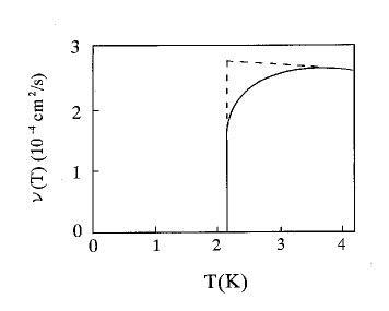
Figure 1: The kinematic viscosity $\nu(T)$ (a solid curve) of a bulk liquid helium 4.

In this paper, the capillary flow above $T_{\lambda}$ is revisited. The two-fluid model, which is the basis for understanding liquid helium 4, separates the system into the normal and superfluid parts from the beginning, and normally assumes that the latter abruptly appears at $T_{\lambda}$. The success of the two-fluid model instilled into us the notion that superflow appears at $T_{\lambda}$ in a mathematically discontinuous manner, and that all anomalous properties above $T_{\lambda}$ are due to thermal fluctuation. (In fact, in liquid helium 4 at $|T/T_{\lambda}-1|<10^{-2}$, the sharp increase in specific heat or the softening of sound propagation arises from thermal fluctuation.) Figure 1 shows the temperature dependence of the kinematic viscosity $\nu(T)=\eta(T)/\rho$ of the capillary flow of liquid helium 4 [8] [9] [10]. In Fig.1, when cooling the system, the kinematic viscosity $\nu(T)$ does not abruptly drops to zero at $T_{\lambda}$ like a dotted line, but it gradually decreases in $T_{\lambda}<T<3.7K$, and finally drops to zero at $T_{\lambda}$. Similarly to the anomalies at $|T/T_{\lambda}-1|<10^{-2}$, this gradual decrease in $\nu(T)$ in $T_{\lambda}<T<3.7K$ has been tacitly attributed to thermal fluctuation (except in ref.8). Actually, behind the two-fluid model, there exists a more basic assumption in statistical physics: the infinite-volume limit. To clearly define the phase transition, this limit eliminates the intermediate-sized order, in which “intermediate size” is equivalent to “microscopic one”. For the mechanical properties, however, in contrast to the thermodynamic ones, one cannot ignore the boundary condition of the system. In particular, in this system, since the size of the coherent wave function and that of the capillary are not so different at low temperatures, we cannot naively use the $V\rightarrow\infty$ limit. Rather, the magnitude of phenomena masked by this limit should be estimated by experiments. (In this sense, the low-temperature phenomenon with quantum coherence is essentially a mesoscopic one.)

Physically, the interpretation of $\nu(T)$ in $T_{\lambda}<T<3.7K$ on the basis of thermal fluctuation is questionable for the following reasons. (1) The range of temperature of 1.5 K from $T_{\lambda}$ to 3.7 K is too large for the thermal fluctuation [11]. For the fluctuation of temperature $\Delta T$, one knows the formula $\langle(\Delta T)^{2}\rangle=k_{B}T^{2}/C_{V}$, in which $C_{V}$ is the heat capacity of a fluctuating small region. As mentioned in ref.8, the $C_{V}$ in the case of $\Delta T=1.5K$ is about $2.8\times 10^{-23}J/K$, which implies that the fluctuating region would have to be as small as one atom diameter. (2) Thermal fluctuation gives rise to the short-lived and randomly oriented wave function obeying Bose statistics. In contrast, for the one-directional flow to show very small shear viscosity [12], a long-lived and coherent translational motion of particles along a specific direction is necessary, which is qualitatively different from thermal fluctuation. (In this sense, the fluctuation-dissipation theorem is not applicable to the nondissipative response such as the decrease in viscosity [13].) Rather, the gradual fall of $\nu(T)$ in $T_{\lambda}<T<3.7K$ is likely to represent the orderly redistribution of particle momenta due to Bose statistics , an advance sign of the state below $T_{\lambda}$ [8].

In the Bose system just above $T_{\lambda}$, particles experience a strong effect of Bose statistics, and the coherent wave function grows to a large but not yet macroscopic size. Since these wave functions are negligible at $V\rightarrow\infty$, they do not affect the definition of phase transition at $T_{\lambda}$. However, in contrast to thermal fluctuation, these intermediate-sized coherent wave functions have a possibility of leading to a coherent translational motion of particles within a mesoscopic distance [14]. At $T_{\lambda}<T<3.7K$, there is no macroscopic condensate connecting the two ends of the capillary, hence no macroscopic frictionless transport occurs. Rather, the intermediate-sized coherent wave function is likely to reduce the $\nu(T)$ of capillary flow. We will call such a wave function mesoscopic condensate not in the thermodynamic sense but in the mechanical sense. Figure.1 must include valuable information on the mesoscopic condensate. Our problem is to estimate it by experiment and compare it with the microscopic model. For this purpose, we must take a somewhat different approach to superflow.

(1) The shear viscosity of a quantum liquid has been studied by applying the kinetic theory of gases to phonons and rotons [15]. However, for our purpose, this method is not applicable. Well below $T_{\lambda}$, various excitations of liquid helium 4 are strictly suppressed except for phonons and rotons. Hence, they are normally regarded as a weakly interacting dilute Bose gas, although the excitation in liquid. For $\nu(T)$ above $T_{\lambda}$, however, the dilute-gas picture has no basis, because the basis for this picture, the macroscopic condensate, has not yet developed. Rather, the strongly interacting excitations in the liquid determine the $\nu$ above $T_{\lambda}$. The effect of Bose statistics on such excitations is worth studying.

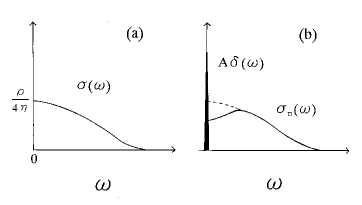
Figure 2: The change of the conductivity spectrum $\sigma(\omega)$ from (a) in a classical fluid to (b) in a superfluid.

In §2, we will develop an alternative method combining the correlation function with fluid dynamics [16]. The distribution of flow velocity in a capillary is described by Poiseuille’s formula

$$v_{x}(r)=\frac{d^{2}-r^{2}}{4\eta}\frac{\Delta P}{L},$$ (1)

where $d$ and $L$ are the radius and length of the capillary, respectively, and $\Delta P$ is the pressure between the two ends of the capillary. The simplest method of measuring $\eta$ is to set the capillary to stand vertically at gravity $g$. The level $h(t)$ of the liquid decreases as $h(t)=h(0)\exp(-\alpha t)$, where $\alpha$ includes $\eta$ as $\rho gd^{4}/(\eta L)$ (see Appendix. A). Hence, $\Delta P(t)$ also decreases as $\Delta P(t)=\Delta P(0)\exp(-\alpha t)$ in eq.(1). In $T_{\lambda}<T<3.7K$, the curve of $h(t)$ shows an anomalously small shear viscosity. Although it shows no sign of frictionless transport, the frequency spectrum of the quantities in eq.(1) reflects the mesoscopic dynamics in the flow as well as the macroscopic one, and therefore, mesoscopic superflow must exhibit a characteristic spectrum in it. On the axis of the capillary ($r=0$), multiplying both sides of eq.(1) by the density $\rho$, we define the massflow density $j(t)=\rho v_{x}(0,t)$, and the conductivity $\sigma=\rho/(4\eta)$. Under an oscillating $P(\omega)\exp(i\omega t)$, the spectrum $j(\omega)$ and $\sigma(\omega)$ (Fig.2(a)) satisfy

$$\mbox{\boldmath$j$}(\omega)=-\sigma(\omega)d^{2}\frac{\Delta\mbox{\boldmath$P$}(\omega)}{L}.$$ (2)

In the capillary flow below $T_{\lambda}$ or in the vicinity of $T_{\lambda}$, the superfluid and normal-fluid parts flow without any transfer of momentum to each other. Accordingly, $\sigma(\omega)$ splits into a sharp peak $A\delta(\omega)$ at $\omega=0$ and a continuous spectrum $\sigma_{n}(\omega)$ as in Fig.2(b);

$$\mbox{\boldmath$j$}(\omega)=-\left[\sigma_{n}(\omega)+A\delta(\omega)\right]d^{2}\frac{\Delta\mbox{\boldmath$P$}(\omega)}{L}.$$ (3)

In §2, eqs.(2) and (3) will be embedded into the general linear-response relation including both the dissipative and nondissipative (dispersive) responses. Applying the Kramers-Kronig relation to them, we will derive a formula of $\nu(T)=1/[4\sigma(T)]$ (eq.(11)) in the vicinity of $T_{\lambda}$, and quantitatively estimate the effect of Bose statistics in Fig. 1. In §2.3, the role of Bose statistics in the fall of shear viscosity will be discussed using the Maxwell relation.

(2) In the microscopic theory of shear viscosity $\eta$, one normally starts from the two-time correlation function of the tensor $J_{xy}(t)=-\sum_{i}(p_{i,x}p_{i,y}/m)$, and perform a perturbation calculation of $\langle J_{xy}(0)J_{xy}(t)\rangle$ with respect to the particle interaction [5] [6]. This method has the following difficulties in solving our problem. In the weak-coupling system (a gas, or a simple liquid such as liquid helium 4), the particle interaction $U$ normally enhances the relaxation of particles to local equilibrium positions in the flow, thereby decreasing $\eta$ [17]. If we would try to formulate this property using the Kubo formula for $\eta$, we must derive the decrease in $\eta$ from the increase in $U$. Since $\eta$ and $U$ changes in opposite directions, there must be a delicate cancellation of higher-order terms in the perturbation expansion of $\eta$. In contrast, when we start from Poiseuille’s formula, in which $\eta$ appears in the denominator of the linear-response coefficient as in eq.(1), we apply the Kubo formula not to $\eta$ but to the reciprocal $1/\eta$ in eq.(2). In the perturbation expansion of $1/\eta$ with respect to $U$, the increase in $U$ naturally leads to the increase in $1/\eta$, and therefore to the decrease in $\eta$ . In this case, one need not expect the cancellation, and the effect of $U$ on $\eta$ is simply built in from the beginning.

(3) We will focus on the redistribution of particle momenta in the vicinity of $T_{\lambda}$. In §3, following ref.14, we assume the Bose system without the macroscopic condensate as a non-perturbed state, and perform a perturbation calculation of $1/\eta$. By taking characteristic diagrams reflecting Bose statistics in the expansion, we will examine how the formation of a larger coherent wave function gradually decreases shear viscosity. Specifically, combining in §3 the phenomenological relation eq.(3) with the microscopic calculation, we will derive the formula of $\sigma(\omega)$ (eq.(28)) illustrated in Fig.2(b) , and derive the suppression of $\nu$.

(4) Compared with macroscopic condensate, the mesoscopic condensate shows different responses in the oscillation experiments. After defining the damping angular frequency (eq.(24)), we will examine the stability of superflow to the oscillation, and estimate the effect of condensate size on the stability (eq.(31)). From this viewpoint, we will briefly discuss the response of the superflow in porous media to torsional oscillation or ultrasound in §4.

Lastly, we will discuss these results in a wider context in §5.

2 Shear Viscosity in Capillary Flow

2.1 Formalism

In classical fluids, the capillary flow is a typical dissipative process. To describe both dissipative and nondissipative processes, let us generalize the conductivity spectrum $\sigma(\omega)$ in eq.(2) to the complex number

$$\mbox{\boldmath$j$}(\omega)=-\left[\sigma_{1}(\omega)+i\sigma_{2}(\omega)\right]d^{2}\frac{\Delta\mbox{\boldmath$P$}(\omega)}{L}.$$ (4)

The spectrum of $\Delta P(t)=\Delta P(0)\exp(-\alpha t)$ is given by $\Delta P(\omega)=\Delta P(0)\pi^{-1}(\omega^{2}+\alpha^{2})^{-1/2}$, which has a peak at $\omega=0$. We define the half width $\omega_{f}$ of the peak as $\omega_{f}=\sqrt{3}\alpha$. In eq.(4), $\sigma_{1}(\omega)$ must satisfy the following sum rule [6] including the conserved quantity $f(d)$ (see Appendix. B)

$$\frac{1}{\pi}\int_{0}^{\infty}\sigma_{1}(\omega)d\omega=f(d).$$ (5)

The average conductivity $\sigma$ is defined as $\sigma=\omega_{f}^{-1}\int_{0}^{\omega_{f}}\sigma_{1}(\omega)d\omega$, hence giving the shear viscosity $\eta=\rho/(4\sigma)$.

To incorporate eq.(4) into the linear-response theory, instead of $\Delta P(\omega)$, we will use the velocity $v_{0}(\omega)$, which satisfies the equation of motion $\rho dv_{0}(t)/dt=-\Delta P(t)/L$. Since $v_{0}(\omega)$ and $j(\omega)$ constitute the perturbation energy $\int j(\omega)v_{0}(\omega)d\omega$, we can regard $v_{0}(\omega)$ as the external field in eq.(4). We rewrite eq.(4) as

$$\mbox{\boldmath$j$}(\omega)=\rho\left[-\omega\sigma_{2}(\omega)+i\omega\sigma_{1}(\omega)\right]d^{2}\mbox{\boldmath$v$}_{0}(\omega),$$ (6)

and regard $\rho\left[-\omega\sigma_{2}(\omega)+i\omega\sigma_{1}(\omega)\right]d^{2}$ as the coarse-grained form of generalized susceptibility. In this formula, the real part $-\omega\sigma_{2}(\omega)$ corresponds to the non-dissipative process, and the imaginary part $\omega\sigma_{1}(\omega)$ to the dissipative one. In liquid, the former corresponds to the Couette flow of viscous liquid in a rotating bucket. When the whole fluid is in the uniform rotation, no internal friction occurs [18], and it rotates like a rigid body as $\mbox{\boldmath$v$}_{d}(\mbox{\boldmath$r$})=\mbox{\boldmath$\Omega$}\times\mbox{\boldmath$r$}$ ($\Omega$ is the angular velocity). The latter corresponds to the capillary flow. They are connected to each other by the Kramers-Kronig relation [19] as

$$\sigma_{1}(\omega^{\prime})=\frac{2}{\pi}\int_{0}^{\infty}d\omega\frac{\omega\sigma_{2}(\omega)}{\omega^{2}-\omega^{\prime 2}}.$$ (7)

Using the response of the rotating liquid as the real part $\omega\sigma_{2}(\omega)$, we can obtain the conductivity of the capillary flow $\sigma_{1}(\omega)$ by eq.(7). $\omega\sigma_{2}(\omega)$ is derived from the susceptibility $\chi_{\mu\nu}(q,\omega)$ (the real part of the generalized one) [20]. In general, the $\chi_{\mu\nu}(q,\omega)$ is decomposed into the longitudinal and transverse parts, $\chi_{\mu\nu}(q,\omega)=\chi^{L}(q,\omega)q_{\mu}q_{\nu}/q^{2}+\chi^{T}(q,\omega)\left(\delta_{\mu\nu}-q_{\mu}q_{\nu}/q^{2}\right)$, in which $\omega\sigma_{2}(\omega)$ belongs to the transverse part. (In the case of the rotation, the effect of the wall of the bucket propagates along the radial direction, which is perpendicular to that of particle motion.) Hence, we rewrite eq.(7) as

$$\rho d^{2}\sigma_{1}(\omega^{\prime})=-\frac{2}{\pi}\int_{0}^{\infty}d\omega\frac{\lim_{q\rightarrow 0}\chi^{T}(q,\omega)}{\omega^{2}-\omega^{\prime 2}}.$$ (8)

In the normal-fluid phase, because of $\chi^{T}(q,\omega)=\chi^{L}(q,\omega)$ for small $q$, $\chi^{T}(q,\omega)$ in eq.(8) is replaced by the longitudinal part $\chi^{L}(q,\omega)$. Such a modified formula with the aid of $\rho=\chi^{L}(q,0)$ defines the normal fluid conductivity $\sigma_{1n}(\omega)$ (see Appendix. B).

As $T\rightarrow T_{\lambda}$, owing to Bose statistics, the energy of the low-lying transverse excitation increases (see §2.3). It destroys the balance between the transverse and the longitudinal excitations, hence $\chi^{L}(q,\omega)-\chi^{T}(q,\omega)\neq 0$ at $\omega\rightarrow 0$. Instead of $\sigma_{1n}(\omega)$ defined by $\chi^{L}(q,\omega)$, one must go back to the original definition of eq.(8), and rewrite it using $\sigma_{1n}(\omega)$ as

$$\sigma_{1}(\omega^{\prime})=\sigma_{1n}(\omega^{\prime})$$ (9)

$$+\frac{2}{\rho\pi d^{2}}\int_{0}^{\infty}d\omega\frac{\lim_{q\rightarrow 0}[\chi^{L}(q,\omega)-\chi^{T}(q,\omega)]}{\omega^{2}-\omega^{\prime 2}}.$$

The integral over $\omega$ in Eq.(9) leads to a sharp peak at $\omega^{\prime}=0$ [19] with the aid of Hilbert transformation as

$$\int_{0}^{\infty}\frac{d\omega}{\omega^{2}-\omega^{\prime 2}}=\frac{\pi^{2}}{2}\delta(\omega^{\prime}).$$ (10)

Accordingly, a sharp peak $\lim_{q\rightarrow 0}[\chi^{L}(q,0)-\chi^{T}(q,0)]\delta(\omega)$ appears in $\sigma_{1}(\omega)$ of eq.(9) as required in eq.(3), where $\lim_{q\rightarrow 0}[\chi^{L}(q,0)-\chi^{T}(q,0)]$ corresponds to the mesoscopic superfluid density $\hat{\rho}_{s}(T)$. Using eq.(10) in eq.(9), and using the result in $\sigma=\omega_{f}^{-1}\int_{0}^{\omega_{f}}\sigma(\omega)d\omega$, we take out the sharp peak from this integral, and obtain the kinematic viscosity $\nu(T)=1/(4\sigma)$ as [21]

$$\nu(T)=\frac{\nu_{n}}{1+\displaystyle{\frac{2\pi}{d^{2}\omega_{f}}\frac{\hat{\rho_{s}}(T)}{\rho}}\nu_{n}},$$ (11)

where $\nu_{n}$ ($=1/[4\sigma_{n}]$) is $\nu$ of the classical liquid.

2.2 Comparison with the experiment

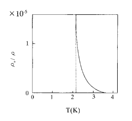
Figure 3: $\hat{\rho}_{s}(T)/\rho$ obtained by eq.(12) using $\nu(T)$ in Fig.1.

Equation (11) is a general formula depending on no specific model of liquids, and we can compare it to $\nu(T)$ shown in Fig.1 [10]. When we view the fall of $\nu(T)$ in Fig.1 as a manifestation of a mesoscopic condensate, we can estimate its $\hat{\rho_{s}}/\rho$ using eq.(11) as follows. We assume $\nu_{n}$ in eq.(11) to be $\nu$ at $T_{on}$=3.7K in Fig. 1, and derive $\omega_{f}$ in eq.(11) from the time dependence of the level of a liquid $h(t)=h(0)exp(-\alpha t)$ as follows. The $\alpha$ of liquid helium 3 was measured at 1.105 K as $5\times 10^{-4}/s$ in Fig.2 of ref.9. At 3.7 K, it approximately changes to $3\times 10^{-4}/s$ with a change of $\rho/\eta$ in $\alpha\propto\rho gd^{4}/(\eta L)$. For liquid heliums 3 and 4 near 3.7 K, the factor $\rho/\eta$ is nearly the same. Hence, we estimate that liquid helium 4 at 3.7 K has $\alpha=3\times 10^{-4}/s$ for a typical size of the capillary, and $\omega_{f}=\sqrt{3}\alpha=5\times 10^{-4}rad/s$ (a small value). With the above $\omega_{f}$ and a typical capillary radius $d=10^{-2}cm$, we estimate $\hat{\rho}_{s}(T)/\rho$ using $\nu(T)$ of Fig.1 as

$$\frac{2\pi}{d^{2}\omega_{f}}\frac{\hat{\rho}_{s}(T)}{\rho}=\nu(T)^{-1}-\nu(T_{on})^{-1},$$ (12)

and obtain Fig. 3. Just above $T_{\lambda}$, $\hat{\rho}_{s}(T)/\rho$ reaches $1.6\times 10^{-5}$.

Compared with the nondissipative process such as the rotation of liquid, the intrinsically dissipative process such as the capillary flow depends on some experimental parameters such as $\omega_{f}$ and $d$ as in eq.(11). In the rotating bucket experiment, the change in the moment of inertia $I_{z}$ simply obeys $I_{z}(T)=I_{z}^{cl}[1-\hat{\rho}_{s}(T)/\rho]$. In the rotation experiment by Hess and Fairbank [22], the moment of inertia $I_{z}$ above $T_{\lambda}$ is slightly smaller than the normal phase value $I_{z}^{cl}$. Using these currently available data, $\hat{\rho_{s}}(T_{\lambda}+0.03K)/\rho\cong 8\times 10^{-5}$, and $\hat{\rho_{s}}(T_{\lambda}+0.28K)/\rho\cong 3\times 10^{-5}$ in ref.14. Despite the subtleness inherent in the dissipative process, $\hat{\rho}_{s}(T)/\rho$ in Fig.3 has the same order of magnitude as $\hat{\rho}_{s}(T)/\rho$ independently obtained using $I_{z}(T)$. Just above $T_{\lambda}$, about $1/10^{5}$ of all helium 4 atoms participate in the mesoscopic condensate. They are negligible in thermodynamic quantities, but manifest themselves in the mechanical response such as shear viscosity. In eq.(11), the effect of $\hat{\rho}_{s}(T)$ is amplified by the small $\omega_{f}$.

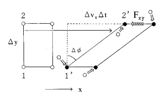
Figure 4: Deformation of a small rectangular element in the flow. The shear stress $F_{xy}$ is expressed as $\eta\partial v_{x}/\partial y$.

2.3 Physical picture in coordinate space

(1) Let us discuss the physical mechanism behind eq.(11). Figure 4 shows a small rectangular element in the flow, which initially deforms macroscopically, then relaxes to a part of the stationary flow with a relaxation time $\tau_{M}$. For $\eta$ of the classical liquid, Maxwell obtained a simple formula $\eta=G\tau_{M}$ (the Maxwell relation) in analogy with solids, where $G$ is the modulus of rigidity [23]. The macroscopic relaxation in Fig.4 is a result of the accumulation of microscopic relaxations by the excited particles. Quantum mechanics states that, in the decay from an excited state with an energy $E$ to a ground state with $E_{0}$, the higher excitation energy $E$ causes a shorter microscopic relaxation time $\tau$ as $\hbar/\tau\simeq|E-E_{0}|$. In eq.(8), the left-hand side includes the $\tau_{M}$ in $\sigma_{1}=\rho/(4G\tau_{M})$, whereas the right-hand side includes the many-body excitation spectrum in $\chi^{T}(q,\omega)$. In this sense, eq.(8) is the many-body version of $\hbar/\tau\simeq|E-E_{0}|$. (In other words, eq.(8) is another expression of the Maxwell relation.) In liquids, slightly different microscopic local structures are irregularly arranged , the energies $E$’s of which differ only slightly from each other. In the relaxation of one arrangement to others, the smaller energy difference $|E-E_{0}|$ leads to a longer $\tau$ in $\hbar/\tau\simeq|E-E_{0}|$. These long $\tau$’s result in a long $\tau_{M}$ of the macroscopic deformation, thus leading to a large shear viscosity $\eta=G\tau_{M}$ of the classical liquid.

In liquid helium 4 near $T_{\lambda}$, no structural transition is observed in coordinate space. Hence, $G$ must be a constant at the first approximation, and therefore the fall of the shear viscosity $\eta=G\tau_{M}$ is attributed to the decrease in $\tau_{M}$. At the microscopic level, this comes from the decrease in $\tau$’s. In view of $\hbar/\tau\simeq|E-E_{0}|$, the decrease in $\tau$ suggests the increase in $E$. Near $T_{\lambda}$, it is natural to attribute it to the effect of Bose statistics. The relationship between the excitation energy and Bose statistics dates back to Feynman’s argument on the scarcity of low-energy excitation in liquid helium 4 [24], in which he explained how Bose statistics affects the many-body wave function in configuration space. We will apply his explanation to the analysis of shear viscosity.

(2) Consider the motion of particles in Fig.4. For example, two particles 1 and 2, each of which simultaneously starts at $(x,y)$ and $(x,y+\Delta y)$, move along the $x$-direction to positions 1’ and 2’. The long thin arrows represent the displacement of white circles to black ones. In the BEC phase, the many-body wave function has permutation symmetry everywhere, and all white circles are therefore permutable in Fig.4. At first sight, these displacements by long arrows seem to be a large change, but they are reproduced by a set of small displacements of neighboring white circles by short thick arrows as shown in Fig.4. In Bose statistics, owing to permutation symmetry, one cannot distinguish between two types of particles after displacement, one moved from near positions by a short arrow, and the other moved from distant initial positions by a long arrow. Even if the displacement made by the long arrows is a large displacement in classical statistics, it is only a small displacement by the short arrows in Bose statistics . The displacement related to shear viscosity is a transverse one. In general, the transverse displacement does not change particle density on a large scale, and therefore, for any given particle after displacement, a nearby particle always exists in the initial distribution. (On the other hand, the longitudinal displacement largely changes the particle density, and therefore nearby particles do not always exist, which implies $\chi^{L}(q,\omega)-\chi^{T}(q,\omega)\neq 0$ in eq.(9).)

Let us consider this situation in 3N-dimensional configuration space following Feynman. The excited state related to shear viscosity, in which particles make small displacements, has a wave function that is not far apart from the ground-state wave function in configuration space. The excited-state wave function must be orthogonal to the ground-state wave function. Since the latter has an uniform amplitude, the former must spatially oscillate between the plus and minus values. This means that the wave function of the excited state due to slight displacements must oscillate within a small distance in configuration space. The kinetic energy of the system is determined by the 3N-dimensional gradient of the many-body wave function, and therefore this steep rise and fall of amplitude raises excitation energy. The relaxation of such a microscopic state is a rapid process. When these processes occur simultaneously, it leads to a rapid relaxation of the macroscopic deformation. This mechanism intuitively explains why Bose statistics leads to the decrease in shear viscosity $\eta=G\tau_{M}$.

(3) When the system is at high temperatures, the coherent wave function has a microscopic size. If the long arrow in Fig.4 takes a particle out of such a wave function, the particle after displacement cannot be reproduced by the slight displacement. The mechanism below $T_{\lambda}$ does not work for such a displacement, and $\tau_{M}$ changes to the ordinary long $\tau_{M}$ in the classical liquid. When the system is in $T_{\lambda}<T<3.7K$, the size of the coherent wave function is mesoscopic. In a repulsive system with high density such as liquid, the large-distance motion takes much energy, and therefore in the low-energy excitation, particles are likely to stay within the same wave function. The energy of such an excitation is low compared with that of the excitation due to large displacements, but owing to Bose statistics, it is not so low as that in the classical liquid, and therefore its relaxation to the ground state is relatively a fast process [12]. As $T\rightarrow T_{\lambda}$, the number of such fast relaxations gradually increases, and the superflow appears within the mesoscopic distance, which is the reason for the substantial fall of $\eta$ at $T_{\lambda}<T<3.7K$.

3 Microscopic Model

3.1 Onset of superflow

To formulate the mechanism of the fall of $\nu$ above $T_{\lambda}$, we consider the repulsive Bose system having the following hamiltonian

$$H=\sum_{p}\epsilon(p)\Phi_{p}^{\dagger}\Phi_{p}+U\sum_{p,p^{\prime}}\sum_{q}\Phi_{p-q}^{\dagger}\Phi_{p^{\prime}+q}^{\dagger}\Phi_{p^{\prime}}\Phi_{p},\qquad(U>0),$$ (13)

where $\Phi_{p}$ is the annihilation operator of a spinless boson, and begin with the state without the macroscopic condensate. The onset of superflow above $T_{\lambda}$ has a similar mechanism to the onset of the nonclassical moment of inertia above $T_{\lambda}$. In this subsection, we recapitulate ref.14 on this point with some modifications.

Let us discuss the role of particle interaction. The susceptibility $\chi_{\mu\nu}(q,\omega)$ is a correlation function of currents $j_{\mu}(q,\tau)=\sum_{p,n}(p+q/2))\Phi_{p}^{\dagger}\Phi_{p+q}e^{-i\omega_{n}\tau}$. From $\chi_{\mu\nu}=\chi^{L}q_{\mu}q_{\nu}/q^{2}+\chi^{T}(\delta_{\mu\nu}-q_{\mu}q_{\nu}/q^{2})$, we will extract the term proportional to $q_{\mu}q_{\nu}$, and define $\hat{\chi}_{\mu\nu}(q,\omega)=(\chi^{L}-\chi^{T})q_{\mu}q_{\nu}/q^{2}$ for $\hat{\rho_{s}}(T)$. In the ideal Bose system, we obtain

$$\hat{\chi}_{\mu\nu}(q,\omega)=-\frac{q_{\mu}q_{\nu}}{4}\frac{1}{V}\sum_{p}\frac{f_{B}(\epsilon(p))-f_{B}(\epsilon(p+q))}{\omega+\epsilon(p)-\epsilon(p+q)},$$ (14)

where $f_{B}(\epsilon(p))$ is the Bose distribution. If bosons would form the macroscopic condensate, $f_{B}(\epsilon(p))$ in eq.(14) is a macroscopic number for $p=0$ and nearly zero for $p\neq 0$. Thus, in the sum over $p$ on the right-hand side of eq.(14), only two terms corresponding to $p=0$ and $p=-q$ remain, with a result of $\hat{\chi}_{\mu\nu}(q,0)=\rho_{s}(T)q_{\mu}q_{\nu}/q^{2}$. When bosons form no condensate, however, the sum over $p$ in eq.(14) is carried out by replacing it with an integral, and one notices that $q^{-2}$ dependence disappears, hence $\rho_{s}(T)=0$. This means that when examining the system near $T_{\lambda}$, $\hat{\chi}_{\mu\nu}(q,\omega)$ under the particle interaction $H_{I}$ is needed. We obtain a perturbation expansion of $\chi_{\mu\nu}(q,\omega)$ with respect to $U$ as

$$\langle G|T_{\tau}j_{\mu}(x,\tau)j_{\nu}(0,0)|G\rangle$$

$$=\frac{\displaystyle{\langle 0|T_{\tau}\hat{j}_{\mu}(x,\tau)\hat{j}_{\nu}(0,0)exp\left[-\int_{0}^{\beta}d\tau\hat{H}_{I}(\tau)\right]|0\rangle}}{\displaystyle{\langle 0|exp\left[-\int_{0}^{\beta}d\tau\hat{H}_{I}(\tau)\right]|0\rangle}}.$$

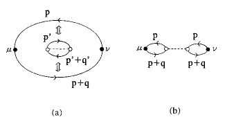
Figure 5: When $p=p^{\prime}$ and $p+q=p^{\prime}+q^{\prime}$ in (a), an exchange of particles between large and small bubbles yield (b).

In eq.(8) and its modified form of $\sigma_{1n}(\omega)$ using $\chi^{L}(q,\omega)$, the characteristic excitations of a liquid is included in $\chi^{L}(q,\omega)$. $\hat{\chi}_{\mu\nu}(q,\omega)=(\chi^{L}-\chi^{T})q_{\mu}q_{\nu}/q^{2}$ represents the change of $\chi^{L}$ induced by Bose statistics. When $\hat{\chi}_{\mu\nu}(q,\omega)$ first obtains a nonzero value at $T_{on}$, one can represent it by the simplest process in eq.(15). Figure. 5(a) shows $j_{\mu}j_{\nu}$ as a large bubble, and the effect of $H_{I}$ as a small bubble with a dotted line $U$. As $T\rightarrow T_{\lambda}$ in the normal phase, Bose statistics forces particles in the large and small bubbles to strictly obey the permutation symmetry. In Fig.5(a), when one of two momenta are equal ($p=p^{\prime}$) for two bubbles, and when the other two momenta are also equal ($p+q=p^{\prime}+q^{\prime}$), a graph made by exchanging these particles must be included in the perturbation expansion. Cutting the line at the point denoted by opposite arrows in Fig.5(a), and reconnecting it to the line with the same momentum of the other bubble yields two bubbles in Fig.5(b) with the common momenta $p$ and $p+q$ connected by the repulsive interaction $U$. As the mesoscopic condensate grows, such an exchange occurs many times, thus leading to a large chain of bubbles. Furthermore, among various momenta, the process including particles with $p=0$ or $p+q=0$ grows to play a dominant role. As a result, we obtain

$$\hat{\chi}_{\mu\nu}(q,i\omega)$$

$$=\frac{q_{\mu}q_{\nu}}{4}\frac{1}{V}\left[\frac{F_{\beta}(q,i\omega)}{1-UF_{\beta}(q,i\omega)}+\frac{F_{\beta}(q,-i\omega)}{1-UF_{\beta}(q,-i\omega)}\right],$$

where

$$F_{\beta}(q,i\omega)=$$

$$\frac{(\exp(\beta[\Sigma-\mu])-1)^{-1}-(\exp(\beta[\epsilon(q)+\Sigma-\mu])-1)^{-1}}{-i\omega+\epsilon(q)}.$$

($\Sigma$ is the self energy and $\mu$ is the chemical potential.) Since our interest is $\chi^{L}-\chi^{T}$ near $\omega=0$, we expand eq.(16) with respect to $\omega$

$$\hat{\chi}_{\mu\nu}(q,\omega)=\frac{q_{\mu}q_{\nu}}{4}\frac{1}{V}\frac{2F_{\beta}(q,0)}{1-UF_{\beta}(q,0)}$$ (18)

$$\times\left[1-\left(\frac{\omega}{\epsilon(q)(1-UF_{\beta}(q,0))}\right)^{2}+\cdots\right].$$

$F_{\beta}(q,0)$ in eq.(17) is a positive monotonically decreasing function of $q^{2}$. Since our interest is the macroscopic response of the system, let us expand it with respect to $q^{2}$ as

$$F_{\beta}(q,0)=\frac{\beta}{4\sinh^{2}\displaystyle{\left(\frac{|\beta[\mu(T)-\Sigma]|}{2}\right)}}$$ (19)

$$\times\left[1-\frac{\beta}{2}\frac{1}{\tanh\displaystyle{\left(\frac{|\beta[\mu(T)-\Sigma]|}{2}\right)}}\frac{q^{2}}{2m}+\cdots\right]$$

$$\equiv a-bq^{2}+\cdots.$$

The denominator on the right-hand side of eq.(18) has the form $1-UF_{\beta}(q,0)=(1-Ua)+Ubq^{2}+\cdots$. As $T$ approaches $T_{\lambda}$ ($\mu(T)-\Sigma\rightarrow 0$), the first term $a$ in the expansion of $F_{\beta}(q,0)$ gradually increases. Hence, $1-Ua$ gradually decreases, and finally satisfies $1-Ua=0$. At this temperature, eq.(18) becomes proportional to $q_{\mu}q_{\nu}/q^{2}$ as $V^{-1}[a/(2Ub)]q_{\mu}q_{\nu}/q^{2}$, hence giving its coefficient $\chi^{L}-\chi^{T}$ a nonzero value. This is a sign of the onset of superflow by the mesoscopic condensate [14].

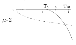
Figure 6: The temperature dependence of $\mu(T)-\Sigma(U)$ depicted by a solid curve, and the condition of eq.(20) by a one-point-dotted one. $T_{on}$ corresponds to 3,7K in Fig.1.

The condition $1-Ua=0$ yields

$$U\beta=4\sinh^{2}\left(\frac{\beta[\mu(T)-\Sigma]}{2}\right).$$ (20)

Figure. 6 schematically shows the condition of eq.(20) by a one-point-dotted curve, and $\mu(T)-\Sigma$ of the system by a thick curve. (The simplest approximation for $\mu(T)$ of liquid helium 4 is to use $\mu(T)$ of the ideal Bose gas with $T_{c}$ replaced with $T_{\lambda}$,

$$\mu(T)-\Sigma(U)=-\left(\frac{g_{3/2}(1)}{2\sqrt{\pi}}\right)^{2}k_{B}T_{\lambda}\left[\left(\frac{T}{T_{\lambda}}\right)^{3/2}-1\right]^{2},$$ (21)

which approximation dates back to London’s paper.) Since $\mu(T)-\Sigma$ reaches zero at the finite temperature $T_{\lambda}$, it approaches zero more rapidly than the one-point-dotted curve by eq.(20). Hence, above $T_{\lambda}$, there is always a temperature in which eq.(20) is satisfied. This is the reason why $\nu(T)$ in eq.(11) begins to fall above $T_{\lambda}$ as in Fig.1. We call this temperature the onset temperature $T_{on}$. Using the definition of $a$ and $b$ in eq.(19) and $Ua=1$ in $V^{-1}[a/(2Ub)]q_{\mu}q_{\nu}/q^{2}$, the mesoscopic superfluid density $\hat{\rho_{s}}(T)=\lim_{q\rightarrow 0}[\chi^{L}-\chi^{T}]$ at $T_{on}$ has the form

$$\hat{\rho_{s}}(T)=\frac{1}{V}\frac{m}{\sinh|\beta[\mu(T)-\Sigma]|}.$$ (22)

Since the sizes of the condensate and capillary are not so different, we do not take the $V\rightarrow\infty$ limit in eq.(22). Hence even when $\mu-\Sigma\neq 0$, $\hat{\rho_{s}}(T)$ is finite. Using eq.(22) in eq.(11), we can describe the fall of $\nu(T)$ in Fig.1. Equation (22) serves as an interpolation formula of $\hat{\rho_{s}}(T)$ in $T_{\lambda}<T<3.7K$, and jumps to a macroscopic value at $T_{\lambda}$.

3.2 Conductivity spectrum

Let us obtain the expression of $\sigma_{1}(\omega)$ in eq.(9). In Fig.2(b), the emergence of the peak at $\omega=0$ is accompanied by a gradual change of the continuum part. At $T=T_{on}$ ($Ua=1$), we rewrite eq.(18) as

$$\hat{\chi}_{\mu\nu}(q,\omega)=\frac{q_{\mu}q_{\nu}}{q^{2}}\frac{a^{2}}{2Vb}\left[1-\frac{\omega^{2}}{\omega_{d}^{2}}+\cdots\right],$$ (23)

where

$$\omega_{d}^{2}=\frac{\epsilon(q_{e})^{4}}{4(k_{B}T)^{2}}\frac{1}{\tanh^{2}\displaystyle{\left(\frac{|\beta[\mu(T)-\Sigma]|}{2}\right)}}.$$ (24)

($q_{e}$ is the wave number representing the size of the capillary.) We want a simple formula of $\hat{\chi}_{\mu\nu}(q,\omega)$ that agrees with eq.(23) at $\omega\rightarrow 0$ and shows a reasonable behavior at $\omega\rightarrow\infty$. At $T_{on}$, the simplest form of $\hat{\chi}_{\mu\nu}=(\chi^{L}-\chi^{T})q_{\mu}q_{\nu}/q^{2}$ satisfying these conditions is given by

$$\hat{\chi}_{\mu\nu}(q,\omega)\simeq\frac{q_{\mu}q_{\nu}}{q^{2}}\frac{a^{2}}{2Vb}\frac{1}{\left(\displaystyle{1+\frac{\omega^{2}}{\omega_{d}^{2}}}\right)}.$$ (25)

Equation.(25) represents the dynamical balance between the longitudinal and transverse responses. Using the definitions of $a$ and $b$ in eq.(19) and $Ua=1$, we define the generalized form of the mesoscopic superfluid density $\hat{\rho_{s}}(T,\omega)\equiv\lim_{q\rightarrow 0}[\chi^{L}(q,\omega)-\chi^{T}(q,\omega)]$ as

$$\hat{\rho_{s}}(T,\omega)=\frac{1}{V}\frac{m}{\sinh|\beta[\mu(T)-\Sigma]|}\frac{1}{\left(\displaystyle{1+\frac{\omega^{2}}{\omega_{d}^{2}}}\right)}.$$ (26)

Using eq.(26) as $\chi^{L}-\chi^{T}$ in eq.(9), taking the finite part of the integral as

$$\int_{0}^{\infty}d\omega\frac{1}{\omega^{2}-\omega^{\prime 2}}\frac{1}{\left(\displaystyle{1+\frac{\omega^{2}}{\omega_{d}^{2}}}\right)}=\frac{-\pi}{2\omega_{d}\left(\displaystyle{1+\frac{\omega^{\prime 2}}{\omega_{d}^{2}}}\right)},$$ (27)

and eq.(24) for $\omega_{d}$, we obtain the real part of conductivity as

$$\sigma_{1}(\omega)=\sigma_{1n}(\omega)+\frac{2V^{-1}}{\rho\pi d^{2}}\frac{m}{\sinh|\beta[\mu(T)-\Sigma]|}\frac{\pi^{2}}{2}\delta(\omega)$$

$$-\frac{2V^{-1}}{\rho\pi d^{2}}\left(\frac{k_{B}T}{\epsilon(q_{e})^{2}}\right)\frac{m}{\displaystyle{\cosh^{2}\left(\frac{|\beta[\mu(T)-\Sigma]|}{2}\right)}}\frac{\pi}{\left(1+\displaystyle{\frac{\omega^{2}}{\omega_{d}^{2}}}\right)}.$$

$\sigma_{1}(\omega)$ must satisfy the sum rule eq.(5) whether it is in the normal or superfluid phases. (In $\int_{0}^{\infty}\sigma_{1}(\omega)d\omega$ of the sum rule, the second term in the bracket of the right-hand side of eq.(28) yields a term proportional to $1/\sinh|\beta[\mu(T)-\Sigma]|$ with the aid of $\int_{0}^{\infty}d\omega/(1+\omega^{2}/\omega_{d}^{2})=\pi\omega_{d}/2$ and eq.(24). The first and second terms in the bracket of eq.(28) cancel out each other in $\int_{0}^{\infty}\sigma_{1}(\omega)d\omega$. [21])

In eq.(28), $\sigma_{1n}(\omega)$ is given by the real part of eq.(B5) in Appendix. B. Hence, the conductivity of the normal-fluid part $\sigma_{n}(\omega)$ is given by

$$\sigma_{n}(\omega)=\frac{1}{\omega d^{2}}Im\left(1-\frac{1}{J_{0}\left(id[1+i]\displaystyle{\sqrt{\frac{\omega}{2\nu_{n}}}}\right)}\right)$$

$$-\frac{2}{nd^{2}}\left(\frac{k_{B}T}{\epsilon(q_{e})^{2}}\right)\frac{V^{-1}}{\displaystyle{\cosh^{2}\left(\frac{|\beta[\mu(T)-\Sigma]|}{2}\right)}}\frac{1}{\left(1+\displaystyle{\frac{\omega^{2}}{\omega_{d}^{2}}}\right)},$$

($J_{0}$ is the zeroth order Bessel function, and $n=\rho/m$). The temperature dependence of $\sigma_{n}(\omega)$ comes from the second term on the right-hand side of eq.(29). As $\mu(T)-\Sigma\rightarrow 0$, $1/\cosh^{2}|\beta[\mu(T)-\Sigma]/2|$ and $\omega_{d}$ increase, hence, $\int_{0}^{\infty}\sigma_{n}(\omega)d\omega$ decreases. On the other hand, the conductivity of the superfluid part $\sigma_{s}(\omega)$ satisfies

$$\int_{0}^{\infty}\sigma_{s}(\omega)d\omega=\frac{\pi}{2nd^{2}}\frac{V^{-1}}{\sinh|\beta[\mu(T)-\Sigma]|}.$$ (30)

As $\mu(T)-\Sigma\rightarrow 0$, the sharp peak at $\omega=0$ increases owing to $1/\sinh|\beta[\mu(T)-\Sigma]|$. Equation (29) and (30) are the simplest formulae describing the change in $\sigma(\omega)$ at $T_{\lambda}<T<3.7K$ in Fig.2.

3.3 Stability of superflow

Equation. (26) implies that, for the objects oscillating at the frequency above $\omega_{d}$, a considerable part of the superfluid behaves as a normal flow. Here, we call $\omega_{d}$ in eq.(24) the damping angular frequency . For the experiment using the vertically standing capillary in gravity, we measure the integrated response of the system from $\omega=0$ to $\omega_{f}$. As long as the properties at approximately $\omega=0$ determine the observed quantities, this feature above $\omega_{d}$ does not seriously affect the result. On the other hand, there is another type of experiment in which the superfluid behavior is measured only at certain frequencies, such as torsional oscillation or ultrasound. In this method, there is a case in which the above feature gives rise to a serious problem (see §4).

The stability of the superflow by the mesoscopic condensate depends on temperature. As the Bose statistical coherence grows in eq.(24) ($\mu(T)-\Sigma\rightarrow 0$), the superflow becomes robust to the oscillating probe in eq.(26) ($\omega_{d}\rightarrow\infty$). By gradually changing temperature at $T>T_{\lambda}$, we can realize different size distributions of the mesoscopic condensate in the capillary flow. The quantity reflecting the size of the condensate is the chemical potential $\mu(T)$. Here, to characterize the size distribution of the condensate at $T$, we use the number of particles $\langle s\rangle$ satisfying $\beta(\mu-\Sigma)\langle s\rangle=-1$ (see Appendix.C). For a small $\mu-\Sigma$, eq.(24) is rewritten as

$$\omega_{d}=\frac{\epsilon(q_{e})^{2}}{k_{B}T}\langle s\rangle.$$ (31)

As $\langle s\rangle$ grows, $\omega_{d}$ increases, hence, as the size of the mesoscopic condensate grows, the superflow by the mesoscopic condensate gradually becomes robust to the oscillating probe.

The stability of superflow is also related to the repulsive interaction $U$. In the famous argument by Landau on the critical velocity of fully developed BEC, the change of one-particle spectrum from $p^{2}/(2m)$ to $v_{s}p$ induced by the repulsive interaction in the Bogoliubov spectrum plays a crucial role [2]. Although Landau’s argument deals with the magnitude of critical velocity, eq.(26) deals with the upper limit of frequency at which flow velocity changes. When $U=0$ in eq.(18), $\hat{\rho_{s}}(T,\omega)$ is written in the form of eq.(26), with $\sinh|\beta[\mu(T)-\Sigma]|$ replaced by $\sinh^{2}(|\beta[\mu(T)-\Sigma]|/2)$. In this case, $\omega_{d}^{2}$ in eq.(24) is simply $\epsilon(q_{e})^{2}$. Hence, with increasing $\omega$, $\hat{\rho_{s}}(T,\omega)$ vanishes far more rapidly than that in the case of $U\neq 0$. Physically, the repulsive interaction $U$ prevents the drop of particles from the superflow, thus stabilizing it. In eq.(24), the repulsive interaction gives the factor $1/\tanh^{2}(|\beta[\mu(T)-\Sigma]|/2)$ to $\omega_{d}^{2}$. Hence, $\hat{\rho_{s}}(T,\omega)$ does not easily vanish for a large $\omega$ in eq.(26). The repulsive interaction plays the significant role not only in the emergence of superflow by mesoscopic condensate, but also in its stabilization. In this sense, eqs.(24) and (26) are extensions of Landau’s argument to the underdeveloped BEC.

4 Implication for Superflow in Porous Media

In the capillary flow above $T_{\lambda}$, the mesoscopic condensate spontaneously emerges in free space, whereas in porous media below $T_{c}$, it is forced to emerge in a restricted space [25]. Despite this difference, when we focus on a single flow through a pore, the result of this paper gives us a simple criterion for the stability of superflow in porous media. In porous media, the superflow is normally measured by the method of torsional oscillation or ultrasound. Just below $T_{c}$, $\langle s\rangle$ in eq.(31) and $\omega_{d}$ in eq.(26) are still small. When the oscillator at $\omega>\omega_{d}$ induces the oscillation of superfluid, $[\hat{\rho_{s}}(T,0)-\hat{\rho_{s}}(T,\omega)]/\hat{\rho_{s}}(T,0)$ of the superfluid behaves as a normal-fluid part. Hence, $\omega^{2}/(\omega^{2}+\omega_{d}^{2})$ of superfluid is locked to the substrate , and $\hat{\rho_{s}}(T)$ is underestimated. With decreasing temperature, this underestimation of $\hat{\rho_{s}}(T)$ is improved by an increase in $\omega_{d}$ [26]. Alternatively, when we change the frequency at a given temperature, the oscillation methods using a higher frequency will detect a larger discrepancy between $T_{c}$ in the mechanical response and $T_{c}$ in the thermodynamic one.

On the other hand, in the oscillation experiments on the superfluid, another type of upper limit $\omega_{p}$ is known, which is set for the normal-fluid part to be locked to the substrate. (The viscous penetration depth $\delta=\sqrt{\nu/(2\omega)}$ must be greater than the channel size. Since the relevant size of the channel is about $10^{-5}cm$ and $\nu\simeq 10^{-4}cm^{2}/s$, $f_{p}=\omega_{p}/2\pi$ is roughly $10^{6}$ Hz.) In normal situations, $\omega_{p}>\omega_{d}$ is usually satisfied. At $\omega>\omega_{p}$, neither the normal-fluid nor superfluid parts is locked to the substrate, hence, $\hat{\rho_{s}}(T)$ is overestimated. At $\omega_{d}>\omega$, the normal and superfluid parts are correctly discriminated. A delicate problem arises at $\omega_{p}>\omega>\omega_{d}$, especially when a frequency comparable to $f_{p}=\omega_{p}/2\pi$ is used in ultrasound. Although $\omega_{p}$ does not depend on temperature, $\omega_{d}$ increases with decreasing temperature, and there may be a case of $\omega_{d}>\omega_{p}$ at very low temperatures. When we represent $\omega_{d}$ by its maximum $\omega_{d}(T=0)$, we can classify the situation into two cases: $\omega_{p}>\omega_{d}(T=0)$ and $\omega_{d}(T=0)>\omega_{p}$, depending on the type of porous medium. The interpretation of the experimental data obtained in such a situation will be complicated, because of the existence of two different kinds of upper limit in frequency.

Recently, a comparison between the measurement using a torsional oscillator (2140 Hz) and by ultrasound (10 MHz) was made in liquid helium 4 confined in a porous substrate, hectorite, and Gelsil [27]. The decoupling of the superfluid from the oscillating substrate results in a decrease in the moment of inertia $\Delta I_{z}$, and in the increase in the ultrasound velocity $\Delta v_{s}$. Different situations will be realized according to different frequencies and substrates. The comparison of experimental data between different frequencies will give us a clue to the dynamics of superflow in porous media.

5 Discussion

5.1 Comparison between superflow in the dissipative process and that in the nondissipative one

On the onset mechanism of superflow, it makes a difference whether superflow appears in the dissipative or nondissipative process. Comparing the moment of inertia $I_{z}(T)=I_{z}^{cl}(1-\hat{\rho_{s}}(T)/\rho)$ for the non-dissipative process [14] with the kinematical viscosity $\nu(T)$ of eq.(11) for the dissipative one, we note the following features of $\nu(T)$.

(1) In $I_{z}(T)=I_{z}^{cl}(1-\hat{\rho_{s}}(T)/\rho)$, $\hat{\rho_{s}}(T)$ appears only in the coefficient of the linear term of $I_{z}^{cl}$. In $\nu(T)$ of eq.(11), the effect of Bose statistics appears in all coefficients of higher-order terms of $\nu_{n}$ except for the first-order one. This feature does not depend on the particular model of a liquid, but on the general argument. (On the other hand, the microscopic derivation of $\nu_{n}$ depends on the model of a liquid.)

(2) In $I_{z}(T)=I_{z}^{cl}(1-\hat{\rho_{s}}(T)/\rho)$, the change in $\chi^{L}(q,\omega)-\chi^{T}(q,\omega)$ directly affects $I_{z}$ without being enhanced, and therefore the observed effect of the finite $\hat{\rho_{s}}(T)$ above $T_{\lambda}$ is very small. In $\nu(T)$ of eq.(11), because of the sharp peak in the dispersion integral in eq.(9), the small change in $\hat{\rho_{s}}(T)$ is strongly enhanced to the observable change in $\nu(T)$.

(3) The existence of $1/d^{2}$ before $\hat{\rho_{s}}(T)/\rho$ in eq.(11) indicates that the narrower capillary shows clearer evidence of frictionless flow. Similarly, the existence of $1/\omega_{f}$ indicates that the choice of experimental procedure, such as the method of applying the pressure between two ends of the capillary, affects the temperature dependence of the $\nu(T)$ of capillary flow. This means that superflow appearing in the dissipative process depends on more variables than that in the non-dissipative one, which is in accordance with the general feature of nonequilibrium phenomena.

5.2 Comparison with thermal conductivity

In liquid helium 4 near $T_{\lambda}$, we know a marked change in another type of conductivity, the anomalous thermal conductivity. Under a given temperature gradient $\nabla T$, the heat flow $Q$ satisfies $Q=-\kappa\nabla T$, where $\kappa$ is the coefficient of thermal conductivity. In the critical region above $T_{\lambda}$ ($|T/T_{\lambda}-1|<10^{-3}$), the rapid rise of $\kappa$ is observed, and finally at $T=T_{\lambda}$, $\kappa$ abruptly jumps to infinity. For $T_{\lambda}<T<3.7K$, however, two kinds of conductivity behave differently. In shear viscosity, the corresponding conductivity $\sigma(T)=1/(4\nu)$ shows a gradual rise, whereas $\kappa(T)$ shows no such rise. This difference is expected for the following reason. The $\kappa$ in thermal conductivity is expressed in terms of the correlation function with a similar structure to the $\eta$ in shear viscosity, but $\kappa$ and $\eta$ are qualitatively different. Although shear viscosity is associated with the transport of momentum (a vector), thermal conductivity is associated with that of energy (a scalar). For the vector field (velocity field), the direction of vectors has a rich variety in its spatial distribution. Among various flow-velocity fields, we can regard the Couette flow rotating like a rigid body in a bucket as the nondissipative counterpart to the capillary flow. On the other hand, for the scalar field (temperature field), the variety of possible spatial distributions is far limited. The flow of heat energy is always a dissipative phenomenon, and there is no nondissipative counterpart. Hence, the formulation using the Kramers-Kronig relation in §2 cannot be applied to the onset of the anomalous thermal conductivity, and no mechanism that amplifies the small $\hat{\rho_{s}}(T)$ is expected. This formal difference between shear viscosity and thermal conductivity is consistent with the experimental difference between $\sigma(T)=1/(4\nu)$ and $\kappa(T)$ at $T_{\lambda}<T<3.7K$.

5.3 Comparison with Fermi liquids

The fall of the shear viscosity in liquid helium 3 at $T_{c}$ is a phenomenon parallel to that in liquid helium 4. The formalism in §2 is applicable to liquid helium 3 as well. For the behavior above $T_{c}$, however, there is a striking difference between liquid helium 3 and 4. The phenomenon occurring in fermions in the vicinity of $T_{c}$ is not the gradual growth of the coherent wave function, but the formation of Cooper pairs by two fermions. (This difference evidently appears in the temperature dependence of specific heat: The $C(T)$ of liquid helium 3 shows a sharp peak at $T_{c}$ without a symptom of its rise above $T_{c}$.) Once Cooper pairs formed, they are composite bosons with a high density at low temperatures, and immediately jump to the superfluid state. Hence, the shear viscosity of liquid helium 3 shows an abrupt drop at $T_{c}$ without a gradual fall above $T_{c}$, like the dotted line in Fig.1.

5.4 Future problems

As $T$ approaches $T_{\lambda}$, eq.(22) becomes insufficient to use as an interpolation formula of $\hat{\rho_{s}}(T)$, because it predicts a far smaller $\hat{\rho_{s}}/\rho$ than that in Fig.3 when eq.(21) is used. This implies that a considerable number of helium 4 atoms with $p\neq 0$ are dragged into the superflow. Owing to the repulsive interaction, particles are likely to spread uniformly in coordinate space. By this feature, particles with $p\neq 0$ are forced to behave similarly to particles with $p=0$. If they move differently from the superflow, particle density becomes locally high, thus increasing interaction energy. This is the reason why a considerable number of particles with $p\neq 0$ participate in the superflow even when it is above $T_{\lambda}$ . This tendency will become apparent as $T\rightarrow T_{\lambda}$. Hence, the observed $\hat{\rho_{s}}(T)$ may be the sum of all $\hat{\rho_{s}}(T)$’s over different momenta. To explain Fig.3 quantitatively, a more realistic model of liquids is needed.

Among all nonequilibrium phenomena in liquids, the capillary flow of liquid helium 4 takes a unique position. When increasing temperature from below to above $T_{\lambda}$, one can see a primitive form of the shear viscosity of liquids in the gradual rise in $\nu(T)$, which arises from the superfluid in such a way that it does not occur in other systems. The emergence of slightly different local structures leads to a long relaxation time $\tau_{M}$, and hence to a finite shear viscosity of liquids. Its study has a possibility of shedding new light on the liquid theory.

In this paper, we used the Poiseuille solution of classical fluid dynamics, and examined the quantum effect appearing in the coefficient of shear viscosity. As an alternative approach, we know the quantum hydrodynamics by Landau [2] [28]. If we consider the shear viscosity at $T_{\lambda}<T<3.7K$ using this approach, it will correspond to the semiclassical solution in quantum hydrodynamics. This will give us interesting problems from practical and formal viewpoints.

Appendix A $h(t)=h(0)\exp(-\alpha t)$

To measure $\eta$, let us set the capillary to stand vertically in gravity $g$, the upper end of which is connected to a reservoir, while the lower end is open to the helium bath (Fig.1 in ref. 8). The mass of liquid passing through the capillary per unit time is $Q=2\pi\rho\int_{0}^{d}rv_{x}(r)dr$, which is given by eq.(1) as

$$Q=\rho\frac{\pi d^{4}}{8\eta}\frac{\Delta P}{L}.$$ (32)

$h(t)$ is the difference between the level inside the reservoir and the level in the bath. In the reservoir with a radius $R$, a mass of liquid $\rho\pi R^{2}h(t)$ flows out through the capillary at a rate of $Q$. In the vertically standing capillary, $\Delta P(t)$ between the above two levels is $\rho gh(t)$ in eq.(A1). $h(t)$ decreases according to

$$\rho\pi R^{2}\frac{dh}{dt}=-\frac{\pi d^{4}}{8\eta}\frac{\rho^{2}g}{L}h,$$ (33)

thereby leading to $h(t)=h(0)\exp(-\alpha t)$ with $\alpha=\rho gd^{4}/(8\eta LR^{2})$.

Appendix B Conductivity Spectrum $\sigma(\omega)$

The Stokes equation under the oscillating pressure gradient $\Delta P\exp(i\omega t)/L$ is written in the cylindrical polar coordinate as

$$\frac{\partial v}{\partial t}=\nu\left(\frac{\partial}{\partial r^{2}}+\frac{\partial}{r\partial r}\right)v+\frac{\Delta P\exp(i\omega t)}{\rho L}.$$ (34)

Velocity has the form

$$v(r,t)=\frac{\Delta P\exp(i\omega t)}{i\omega\rho L}+\Delta v(r,t),$$ (35)

under the boundary condition $v(d,t)=0$. In eq.(B1), $\Delta v(r,t)$ satisfies

$$\frac{\partial\Delta v(r,t)}{\partial t}=\nu\left(\frac{\partial}{\partial r^{2}}+\frac{\partial}{r\partial r}\right)\Delta v(r,t),$$ (36)

which solution is written in terms of the Bessel function $J_{0}(i\lambda r)$ with $\lambda=(1+i)\sqrt{\omega/(2\nu)}$. Hence,

$$v(r,t)=\frac{\Delta P\exp(i\omega t)}{i\omega\rho L}\left(1-\frac{J_{0}(i\lambda r)}{J_{0}(i\lambda d)}\right).$$ (37)

Using $v(r=0,t)$ of eq.(B4), the conductivity spectrum $\sigma(\omega)$ satisfying $\rho v(0,t)=\sigma(\omega)d^{2}\Delta P\exp(i\omega t)/L$ (eq.(2)) is given by

$$\sigma(\omega)=\frac{1}{i\omega d^{2}}\left(1-\frac{1}{J_{0}\left(id[1+i]\displaystyle{\sqrt{\frac{\omega}{2\nu}}}\right)}\right).$$ (38)

The real part of eq.(B5) gives a curve of $\sigma(\omega)$ in Fig.2(a). (Re $\sigma(0)$ in eq.(B5) agrees with $\rho/(4\eta)$.) It also determines the conserved quantity $\pi^{-1}\int\sigma(\omega)d\omega=f(d)\propto d^{-2}$ in eq.(5).

Appendix C Size of the Condensate

The grand partition function of the ideal Bose system $Z_{0}(\mu)=\prod(1-\exp[\beta(\epsilon_{p}-\mu)])^{-1}$ was rewritten by Feynman and Matsubara in terms of the size distribution of the coherent wave function [29]. For the repulsive Bose system with $\mu(T)-\Sigma$, it is given by

$$Z(\mu)=$$

$$\exp\left[\sum_{s=1}^{\infty}\left(\frac{\exp[\beta(\mu-\Sigma)s]}{s}+A_{s}\frac{V}{\lambda^{3}}\frac{\exp[\beta(\mu-\Sigma)s]}{s^{5/2}}\right)\right],$$

where $s$ is the number of Bose particles participating in the coherent many-body wave function, $\lambda$ is the thermal wavelength, and $A_{s}$ is a weakly $s$-dependent factor. The first and second terms in the exponent of eq.(C1) come from $p=0$ and $p\neq 0$ bosons, respectively. In $\exp[\beta(\mu-\Sigma)s]/s$ of the first term, $1/s$ is a symmetry factor, and $\exp[\beta(\mu-\Sigma)s]$ represents the probability that the condensate has $s$ particles. In $\exp(-\beta|\mu-\Sigma|s)$, the particle number $\langle s\rangle$ satisfying $\beta(\mu-\Sigma)\langle s\rangle=-1$ gives us a rough estimate of the typical volume size of the condensate.

References

- [1] P. Kapitza, Nature,141, (1938) 74, J.F. Allen and A.D. Meissner, Nature, 141, (1938) 75
- [2] L.D. Landau, J.Phys.USSR.5, (1941) 71. F. London Superfluid, (John Wiley and Sons, New York, 1954) Vol.2.
- [3] J.D. Reppy, J. Low. Temp. Phys. 87, (1992) 205.
- [4] Despite the long history of the study of superflow, it is only recently that experiments for the direct confirmation of the flow pattern below have started using the visualization technique (PIV). T. Zhang and S.W. Van Sciver, Nature Phys. 1, (2005) 36, and references therein.
- [5] As a text, G.F. Mazenko, Nonequilibrium Statistical Mechanics, (Wiley-VCH, 2006).
- [6] M.S. Green, J. Chem. Phys.22, (1954) 398, R. Kubo, J. Phys. Soc. Japan.12, (1957) 570, H. Mori, Phy. Rev. 112, (1958) 1829. E. Helfand, Phy. Rev. 119, (1960) 1, J.M. Luttinger, Phy. Rev. 135, A (1964) 1505.
- [7] As an early reference, J. Frenkel, Kinetic Theory of Liquids (Oxford, London, 1946). As a review, T. Keyes, J. Phys. Chem. A 101, (1997) 2921.
- [8] R. Bowers and K. Mendelssohn, Proc. Roy. Soc. Lond. A, 204,(1950) 366. They pointed out that the fall of in does not come from thermal fluctuations, but from the redistribution of the velocity spectrum preceding the transition.
- [9] K.N. Zinoveva, Zh. Eksp. Teor. Fiz, 34, (1958) 609 [Sov. Phys-JETP, 7, (1958) 421]
- [10] C.F. Barenghi, P.J. Lucas, and R.J. Donnelly, J. Low. Temp. Phys. 44, (1981) 491.
- [11] The ideal Bose gas shows infinite fluctuations of the number of particles at . But one cannot naively expect that the actual interacting Bose systems also show large fluctuations in the especially wide range of temperature near .
- [12] In Fig.1, is already times smaller than the of an ordinary classical liquid.
- [13] If increases in the vicinity of , thermal fluctuation seems to be a natural interpretation, because the critical slowing down is likely to enhance the viscosity.
- [14] S. Koh, Phy. Rev.B. 74, (2006) 054501. The intermediate-sized wave function has a possibility of decreasing the moment of inertia above . (For the Meissner effect of a charged Bose gas above , S. Koh, Phy. Rev.B. 68, (2003) 144502.)
- [15] L.D. Landau and I.M. Khalatonikov, JETP 19, (1949) 637, JETP 19, (1949)709, in Collected papers of L.D. Landau, edited by D. ter. Haar (Pergamon, London, 1965).
- [16] L.P. Kadanoff and P.C. Martin, Ann.Phys. 24, (1963) 419.
- [17] In the strong-coupling system, the strong interaction disturbs the relaxation, thereby leading to a large .
- [18] For the rigid-body rotation , the dissipation function is zero at every , where . Although this flow is unstable due to the absence of an energy barrier in an actual viscous liquid, it is intrinsically nondissipative in an ideal circumstance.
- [19] This method originated in the studies of the responses of superconductors. The Meissner effect and the electrical conductivity is described by the real and imaginary parts of the generalized susceptibility, respectively. R.A. Ferrell and R.E. Glover, Phy.Rev,109, (1958) 1398, M. Tinkham and R.A. Ferrell, Phy.Rev.Lett,2, (1959) 331.
- [20] As a review, P. Nozieres, in Quantum Fluids , ed by D.E. Brewer (North Holland, Amsterdam, 1966) p1, G. Baym, in Mathematical methods in Solid State and Superfluid Theory ed by R.C. Clark and G.H. Derrick (Oliver and Boyd, Edingburgh, 1969) p121.
- [21] In eqs.(11),(28) and (30), is used.
- [22] G.B. Hess and W.M. Fairbank, Phy.Rev.Lett,19, (1967) 216.
- [23] J.C. Maxwell, Phil.Trans.Roy.Soc.157, (1867) 49 in The scientific papers of J.C.Maxwell, edited by W.D. Niven (Dover, New York, 2003) vol.2, 26.
- [24] R.P. Feynman, in Progress in Low Temp Phys. vol.1, ed by C.J. Gorter (North-Holland, Amsterdam, 1955) p17.
- [25] Y. Nakamura and T. Takagi, J.Phys.Soc.Jpn.77, (2008) 034608.
- [26] In practice, there remains a locked fraction of superfluid to substrates, which is independent of temperature and frequency, and is relevant to internal geometries of cells.
- [27] J. Taniguchi, H. Ichida, Y. Aoki, S. Fukazawa, M. Hieda, and M. Suzuki, J. Low. Temp. Phys.148, (2007) 791, T. Kobayashi, J. Taniguchi, M. Suzuki, and K. Shirahama, J. Low. Temp. Phys.148, (2007) 797.
- [28] K. Miyake and K. Yamada, Prog.Theor.Phys.57, (1977) 1133.
- [29] R.P. Feynman, Phy.Rev.91, (1953) 1291. T. Matsubara, Prog.Theor.Phys.6, (1951) 714.