Multiband Hamiltonians of the Luttinger-Kohn Theory and Ellipticity Requirements

Abstract

Modern applications require a robust and theoretically strong tool for the realistic modeling of electronic states in low dimensional nanostructures. The $k\cdot p$ theory has fruitfully served this role for the long time since its creation. During last two decades several problems have been detected in connection with the application of the $k\cdot p$ approach to such nanostructures. These problems are closely related to the violation of the ellipticity conditions for the underlying system, the fact that until recently has been largely overlooked. We demonstrate that in many cases the models derived by a formal application of the Luttinger-Kohn theory fail to satisfy the ellipticity requirements. The detailed analysis, presented here on an example of the $6\times 6$ Hamiltonians, shows that this failure has a strong impact on the physically important properties conventionally studied with these models.

The effective mass theory is one of the fundamental parts in the physics of nanostructures. This theory allows us to get theoretical insight into the electronic properties of dominating bands near the extremum points Bir and Pikus (1974); Chuang (1995). Futhermore, the theory establishes a robust computational framework for simulating observable quantum-mechanical states and corresponding energies in the low-dimensional systems including quantum wells, wires, nanodots. In the original Luttinger–Kohn work Luttinger and Kohn (1955) authors applied the theory to the Schrödinger equation perturbed by a smooth potential and constructed a representation for valence bands Hamiltonian near high symmetry point $\Gamma$ of the first Brillouin zone in bulk Zinc-Blende (ZB) crystals with large fundamental band gap. Soon after that, Kane showed how to expand the model to the narrow gap materials such as InSb and Ge for instance, where one can also account for the influence of the conduction bands Kane (1957). One of the advantages of the $k\cdot p$ theory is in its universality. Indeed, the theory had also been extended to cover Wurtzite (WZ) type of crystals, materials with inclusions, heterostructure materials and superlatices Xia (1991). Another advantage of the effective mass theory that has recently been explored in some details in Patil and Melnik, 2009 is its flexibility, as one can easily adjust the models to include additional effects like strain, piezoelectricity, magnetic field, and respective nonlinear effects. These inbuilt multi-scale effects are crucial for such applications as light-emission diodes, lasers, high precision sensors, photo-galvanic elements, hybrid bio-nanodevices, and many others de Abajo (2007).

For a wide range of applications these models have provided good, computationally feasible and efficient approximations that agree well with experimental results Chuang (1995, 2009). However, for some types of crystal materials band structure calculations based on such multiband models lead to the solutions with unphysical properties Smith and Mailhiot (1986); Szmulowicz (1996) or so called spurious solutions Foreman (2007); Yang and Chang (2005); Lassen et al. (2009).

As a result, there have been various attempts to explain the origin of the spurious solutions and develop some reliable procedures on how to avoid them Veprek et al. (2007). These approaches rely on three main ideas: (a) to modify the original Hamiltonian and remove the terms responsible for the spurious solutions Kolokolov et al. (2003); Yang and Chang (2005), (b) to change band-structure parameters Eppenga et al. (1987); Foreman (2007), and (c) to identify and exclude physically inadequate observable states Kisin et al. (1998). All mentioned approaches suffer from the common weakness – the lack of clear justification of the underlying theoretical procedure and thus from limitations in their applicability Veprek et al. (2007, 2008).

In this work we show that spurious solutions are not just a reason but rather an imminent consequence of another fundamental problem in applications of the classical theory – the non-ellipticity of the multiband Hamiltonian. The widely adopted effective mass approximations of the original Schrödinger elliptic Hamiltonian turns out to be non-elliptic for a broad class of known material parameters (cf. Table 1). This fact leads to the following consequence: since any qualitative approximation methods must preserve the topological structure of the spectrum of a general linear operator, and as an implication symmetric properties in case of Schrödinger Hamiltonian, this evident discrepancy signifies the mathematical invalidity of performed approximation procedures for those materials. Among these mutiband Hamiltonians there are a number of widely used $6\times 6$ and $8\times 8$ Hamiltonians.

The paper is organized as follows. First, we revise basic properties of the original Schrödinger equation, and outline the mathematical model of the electronic band-structure problem.

Next, we derive the exact constraints on the material parameters for typical $6\times 6$ Hamiltonians in ZB Luttinger and Kohn (1955); Kane (1957) and WZ Bir and Pikus (1974) materials. Direct calculations using conventional Luttinger parameters (e.g. Madelung et al., 2002; Madelung, 2004) show that such parameters (e.g. Table 1) for many important semiconductor materials entail the violation of ellipticity requirements. As a result, the corresponding bandstructure model for them potentially susceptible to unphysical solutions, even in the bulk case, and therefore ought to be modified. Moreover, the corresponding time dependent Schrödinger equation loses the fundamental property of state conservation Berestetskii et al. (1982).

The material properties (such as fundamental band-gaps and spin-orbit splitting energies) obtained experimentally, represent real phenomena, whereas models based on finite bands Hamiltonians are meant to approximate them. The very last step in such approximation schemes Eppenga et al. (1987) enables us to calculate interband corrections to the main part of the Hamiltonians with help of perturbation theory Luttinger and Kohn (1955); Luttinger (1956); Bir and Pikus (1974). However, this last step lacks a rigorous theoretical foundation as it does not guaranty the convergence of the perturbation expansion. The result is that the derived Hamiltonian, although directly based on experimental parameters (column 4, 1), represents a totally different mathematical object compared to its origin. The physical evidences, to support this claim have been already known for GaAs Pfeffer and Zawadzki (1990) and recently been reported for Si Dorozhkin (2008).

We start with the Schrödinger equation with the potential $V(x)$

$$H_{0}\psi(x)\equiv\frac{\mathbf{p}^{2}}{2m^{\star}}\psi(x)+(V(x)+E^{\star}_{0})\psi(x)=E\psi(x),$$ (1)

where $E^{\star}_{0}$ is the band edge energy of the system, $\mathbf{p}$ is a momentum operator, $x\in\Omega\subset{\mathbb{C}}^{n},n\leq 3$, $m^{\star}$ is a piecewise-constant effective mass parameter. In $\Omega$ we supplement (1) by usual Dirichlet conditions on the boundary $S\equiv\partial\Omega$

$$\psi(x)=0,\quad x\in S.$$ (2)

Our major focus is on the heterostructure case, where the difference in the effective mass and probability current conservation imposes the discontinuity of $\nabla{\psi(x)}$ on the interface between materials (assuming that the basis Bloch functions are the same in all constituents Burt (1999)). In this case an appropriate choice of the functional space for coefficients from (1) is the Hilbert space of distributions with the compact support $\mathcal{H}^{1}(\Omega)$ Hörmander (1983a, b).

Then, the operator $H_{0}$ with the domain of definition $D(H_{0})\subset\mathcal{H}^{3}(\Omega)$ is a symmetric operator with an existing self-adjoint extension, hence it conserves the probability current Dirac (1981). General theory of elliptic partial differential equations characterizes the problem (1) in terms of the corresponding Fredholm type theorems (e.g. Egorov and Shubin, 1998 ), so that the problem (1), (2) has a countable set of eigenvalues $E_{i}$, smallest eigenvalue $E_{0}$ is simple and corresponding eigenstate $\psi_{0}$ is of constant sign in $\Omega$, furthermore

$$E_{i}\in[\rho_{0},\infty),\ \rho_{0}=E^{\star}_{0}+\min\{0,\inf_{\Omega}{V(x)}\},\quad i=0,\ldots n,$$

where V(x) is real.

If $V(x)$ is a gently varying function over the unit cell in the sense of Luttinger and Kohn, 1955 the original operator $H_{0}$ can be approximated by another operator $H$ (using Bloch theorem), determined by the projection $P$ of $H_{0}$ on the considered eigenspace and Lowding perturbation theory Luttinger and Kohn (1955); Bir and Pikus (1974). The last step in this approximation procedure accounts for the influence of the elements from the space complement to the egeinspace by the formula

$$H=PH_{0}+\sum\limits_{i=1}^{r}\lambda^{r}H^{(r)}$$ (3)

up to the order $r$. Setting $\lambda=1$ leads one to the final approximation, under the assumption that the series (3) is convergent for such $\lambda$. Despite a wide applicability of such approximations, the intrinsic ellipticity requirements for the realizations of $H$ have not been explicitly verified in a systematic manner (see Luttinger and Kohn, 1955; Luttinger, 1956; Kane, 1957; Bir and Pikus, 1974; Chuang, 1995, as well as more recent works).

As an example, let us consider two classical Hamiltonians for ZB Luttinger and Kohn (1955) and WZ Bir and Pikus (1974) type of materials with more scrutiny. In what follows we use the parameter notation identical to the works where corresponding Hamiltonians were obtained. When necessary, the parameters will be converted from one notation to another by using the formulas from [p. 82, Yu and Cardona, 2005].

First consider the Luttinger-Kohn (LK) Hamiltonian from Luttinger and Kohn, 1955

$$H^{LK}\equiv\left(\begin{array}[]{ccccccc}\frac{1}{2}P&L&M&0&i\frac{1}{\sqrt{2}}L&-i\sqrt{2}M\\ {L}^{\star}&\frac{1}{6}P+\frac{2}{3}Q&0&M&-\frac{i}{3\sqrt{2}}(P-2Q)&i\sqrt{\frac{3}{2}}L\\ {M}^{\star}&0&\frac{1}{6}P+\frac{2}{3}Q&-L&-i\sqrt{\frac{3}{2}}{L}^{\star}&-\frac{i}{3\sqrt{2}}(P-2Q)\\ 0&{M}^{\star}&-{L}^{\star}&\frac{1}{2}P&-i\sqrt{2}{M}^{\star}&-\frac{i}{\sqrt{2}}{L}^{\star}\\ -\frac{i}{\sqrt{2}}{L}^{\star}&\frac{i}{3\sqrt{2}}(P-2Q)&i\sqrt{\frac{3}{2}}L&i\sqrt{2}M&\frac{1}{3}(P+Q)&0\\ i\sqrt{2}{M}^{\star}&-i\sqrt{\frac{3}{2}}{L}^{\star}&\frac{i}{3\sqrt{2}}(P-2Q)&\frac{i}{\sqrt{2}}L&0&\frac{1}{3}(P+Q)\\ \end{array}\right),$$

where each of the $P,Q,L,M$ is a second order position dependent differential operator or equivalently second order polynomial in the momentum representation Luttinger and Kohn (1955):

$$\begin{array}[]{c}P=(A+B)k_{+}k_{-}+2Bk_{z}^{2},\quad Q=Bk_{+}k_{-}+Ak_{z}^{2},\\[11.0pt] M=\frac{1}{2\sqrt{3}}((A-B)(k_{x}^{2}-k_{y}^{2})-2iCk_{x}k_{y}),\\[11.0pt] L=-i\frac{C}{2\sqrt{3}}k_{-}k_{z},\quad k_{\pm}=k_{x}\pm ik_{y}.\end{array}$$

Our aim is to check the type (elliptic, hyperbolic or essentially hyperbolic) of the $H^{LK}$ as a partial-differential operator (PDO) on $\mathcal{H}^{1}(\Omega)$ as we know that the given Schrödinger operator from (1) is elliptic. Only the second order derivative terms are playing the dominant role in the following analysis because contributions from the terms linear in $k$ as well as from the potential, are bounded in the domain $D(H^{LK})$ Hörmander (1983b). It means that the results for more complicated physical models with potential contributions from additional fields (e.g. strain, magnetic field, etc.) will stay the same as for the original $H^{LK}$, analyzed here. The fact that the Hamiltonian is a linear operator guarantees that it is also true for any other representation of $H^{LK}$ obtained by linear (basis) transformations.

In a more general sense, for any $m$–dimensional matrix PDO $H=\{h_{ij}\}_{i,j=1}^{m}$, where each element $h_{ij}$ is a second order one dimensional PDO Egorov and Shubin (1998); Hörmander (1983a)

$$h_{ij}=\sum\limits_{k,l=0}^{n}h_{ij}^{kl}\frac{\partial^{2}}{\partial x_{k}\partial x_{l}},$$ (5)

the associated quadratic form is defined by

$$G(\xi_{1},...,\xi_{nm})=vMv^{T},\quad v=\left(\xi_{1},\ldots,\xi_{nm}\right),$$ (6)

where $M$ is an $mn\times mn$ matrix composed from the elements $h_{ij}^{kl}$. The $\mathrm{k\cdot p}$ Hamiltonians in $\mathbb{R}^{3}$ are a special case of (5)-(6) with the real eigenvalues $\alpha_{i}$ and $n=3$ (e. g. Veprek et al., 2007).

Using these notations, the procedure of obtaining the ellipticity condition for $H$ reduces to the question about the sign of $\lambda_{i}$ for the associated $M$. More precisely, the matrix differential operator $H$ will be elliptic if and only if all eigenvalues of the corresponding Hermitian $M$ will have the same sign Hörmander (1983b); Egorov and Shubin (1998).

In general, it is a challenging task to calculate the eigenvalues of $M$ explicitly, even for such small as $3\times 3$ Hamiltonians, but we recall that we deal here with usually sparse, band structure operators.

Taking into account the fact that the sequence of eigenenergies of $H_{0}$ is semi-bounded, for an approximation $H^{LK}$ (in the momentum representation), we obtain

$$\lambda_{i}<0,\quad\forall\ i=0,1,\ldots,nm.$$ (7)

The last constrains guarantee the ellipticity (in strong sense Hörmander (1983a)) of Hamiltonian $H$. The operator $H$ possess a self-adjoint extension in $D(H)\subset\mathcal{H}^{k+2}(\Omega)$, $k>0$, provided that the domain $\Omega$ is sufficiently smooth (piecewise Lipschitz). Then it can be extended to a Hermitian operator by closure in the norm [p. 113, Egorov and Shubin, 1998] or via Lax-Miligram procedure Hörmander (1983b). From the physical point of view the smoothness characteristics of $D(H)$ fulfill the natural assumption of quantum theory that the state of the system must be a continuous function of spatial variables even when some coefficients of $H$ have finite jumps like in the heterostructures consisting of different materials Chuang (1995); Burt (1999).

Table 1: The material parameters for ZB type of materials, $d$ – distance from the point $(A,B,C)$ to the ellipticity region $\Lambda_{-}(H^{LK})$

El.	$A$	$B$	$C$	$d$	El.	$A$	$B$	$C$	$d$
AlAs	-7.5	-2	8.4	1.97	Ge	-30	-4.6	33	10.64
AlP	-3.8	-3.4	7.2	0.92	Ge	-30	-4.6	33	10.64
AlP	-3.7	-3.4	7.2	1.01	Ge	-30	-4.4	36	11.99
GaN	-7.5	-3.8	6.1	In	InP	-11	-1.8	10	2.86
C	-4	-3.4	6.6	0.42	InP	-15	-2.1	17	5.72
C	-2.9	-2.3	3.9	In	InP	-9	-3.3	9.6	1.34
C	-6	-3.8	6	In	InSb	-100	-4	96	39.35
C	-3.1	-1.7	0.9	In	InSb	-100	-3	96	40.25
GaAs	-16	-2	6	0.89	Si	-6	-3.5	9.6	1.18
GaAs	-17	-2.2	6.6	0.98	Si	-5.5	-3.6	8.4	0.54
GaAs	-15	-3.1	17	4.83	Si	-6	-3.4	8.4	0.72
GaP	-6	-3	7.2	0.54	SiC	-2.6	-1.7	4.2	0.38
GaP	-8	-2.2	10	2.50	SiC	-4.8	-1.8	5.1	0.67

,

The direct calculation by (6) for $H^{LK}$ ($n=3$, $m=6$) leads us to the $18\times 18$ matrix $M^{LK}$ with the following distinct eigenvalues:

$$\begin{array}[]{cc}\lambda_{1}=-{\frac{\mathit{C}}{2}}+\mathit{A},&\lambda_{2/3}=({\frac{1}{4}}\pm{\frac{\sqrt{3}}{4}})\mathit{C}+\mathit{A},\\[12.0pt] \lambda_{4/5}=\pm{\frac{\mathit{C}}{2}}+\mathit{B},&\lambda_{6/7}={\pm\frac{\mathit{C}}{4}}+\mathit{B},\end{array}$$ (8)

where $\lambda_{1}$, $\lambda_{2/3}$, $\lambda_{4/5}$ have the multiplicity 2 and $\lambda_{6/7}$ have the multiplicity 4, respectively, and $A,B,C$ are usual material parameters Luttinger and Kohn (1955). By substituting (8) into (7), we receive the system of linear inequalities with respect to $A$, $B$ and $C$. They describe the feasibility region in the $A,B,C$ space, when $H^{LK}$ is an elliptic partial differential operator with the discrete and decreasing sequence of eigenvalues. One can use similar reasoning to obtain corresponding inequalities for other common representations of $H^{LK}$ through Luttinger parameters $\gamma_{i}$ Chuang (1995); Bir and Pikus (1974). Evidently, any solution of (7) for (8) would have a unique corresponding solution in $\gamma_{i}$ notation. Note next that the solution domain $\Lambda_{-}(H^{LK})$ of (8), (7) is symmetric with respect to the sign of $C$. It follows from the form of the $H^{LK}$ which is dependent on $|C|$ only. $\Lambda_{-}(H^{LK})$ comprises an unbounded pyramid in $\mathbb{R}^{3}$ (cf. Fig. 1) with the following rays as its edges: $\left(-\frac{1}{2}t,-\frac{1}{2}t,-t\right),\ \left(-\left(\frac{1}{4}+\frac{\sqrt{3}}{4}\right)t,-\frac{1}{2}t,t\right),$ and $(-t,0,0),\ \left(0,-\left(\frac{3}{4}+\frac{\sqrt{3}}{4}\right)t,0\right),$ for $t\in[0,\infty)$.

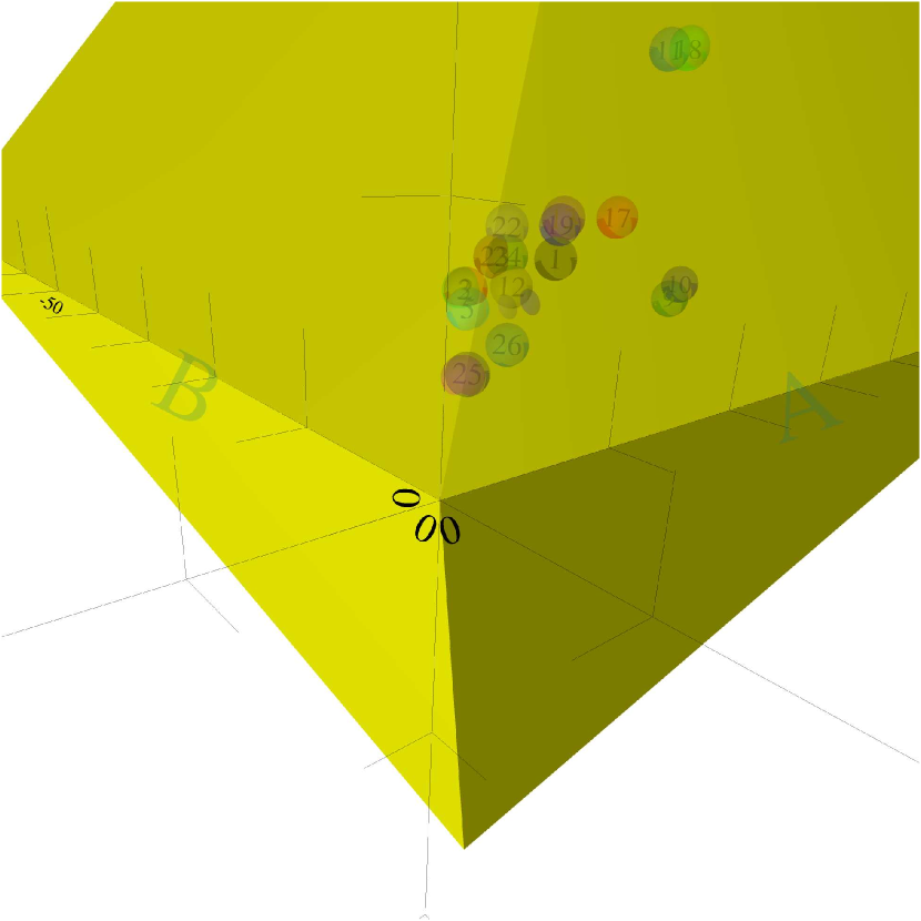
[ poster, toolbar, label=temp, text=, 3Droo=0.2233495084617366, 3Daac=60, 3Dcoo=0.0000067046325966657605 0.011743400245904922 -0.059044793248176575, 3Dc2c=0.060472868382930756 -0.054119743406772614 0.9967015981674194, 3Droll=44.09483043248314, 3Dlights=Hard, 3Dviews2=views.3dv, ]ZBLKinABC.u3d

Figure 1: The region $\Lambda_{-}(H^{LK})$ and the material parameters from Table 1.(color online)

Figure 1 represents the $H^{LK}$ ellipticity region together with the widely adopted values of the material parameters for different ZB type materials summarized in Table 1.

One can observe that, among all analyzed materials only two (indicated as ”In” in the third column of Table 1) have the admissible sets of parameters. All other data from Table 1 yield the condition $\lambda_{4}>0$. That is why the $H^{LK}$, for the corresponding materials, is not elliptic and may not be even symmetric. Moreover, instead the domain $D(H^{LK})=D(H)\subset\mathcal{H}^{3}(\Omega)$ we have only

$$D(H^{LK})=D(H)\subset\mathcal{H}^{1}(\Omega),$$ (9)

it means that the solution of (1) will have the discontinuities, for the systems with jump discontinues coefficients, which is the case for heterostructure materials, see e.g. Courant and Lax, 1956. The general theory guaranties that, in this case, the interface discontinuities will be observed all through the interior of the active region along the characteristics of $H^{LK}$, which are now shown to exist since the associated $G$ in (6) is of nonconstant sign [p. 153, Egorov and Shubin, 1998]. Additionally, (9) and the double degeneracy of $\lambda_{4}$ (8) would lead to the nonanalytic solution and thus the momentum operator, from (1), will be ill-defined (by the embedding theorems, [p. 119, Egorov and Shubin, 1998]). All the arguments stated before allow us to conclude that the $H^{LK}$ does not provide a sufficiently good approximation, preserving the type of the PDO, for most of the practical data.

The ellipticity analysis for ZB, can be applied to a WZ $6\times 6$ Hamiltonian Bir and Pikus (1974); Suzuki et al. (1995) without any changes. Ellipticity conditions that follows from such analysis are, again, linear in parameter variables

$$\begin{array}[]{cc}A_{2}+A_{4}<0,&A_{2}\pm(2A_{5}-2A_{4})<0,\\[12.0pt] A_{2}+4A_{5}<0,&A_{2}+3A_{4}-2A_{5}<0.\end{array}$$ (10)

Namely, $A_{i}$ are well-known Luttinger-like parameters for WZ Bir and Pikus (1974). As in the ZB case, each separate inequality has been obtained from (7) by substituting every distinct eigenvalue of the matrix $M$ associated with the WZ Hamiltonian. These conditions are also violated in most of practically important materials, among which, we would like to mention GaN, AlN and ZnO. Here, the distances to the WZ ellipticity region defined by (10) are approximately equal: 0.804, 0.862, 0.606 for GaN parameter sets Suzuki et al. (1995); Chuang and Chang (1996); Mireles and Ulloa (2000); 1.132 Suzuki et al. (1995); Chuang and Chang (1996), 1.271 Mireles and Ulloa (2000), 1.01 Jeon et al. (1996) for AlN; 1.067 Fan et al. (2006) for ZnO. The distances have the order of terms in the unperturbed part of the WZ Hamiltonian (which in the dimensionless Luttinger-like notation equal to 1), and thus are considerably high.

Let us return back to the feasible parameters for two materials C and GaN. For carbon, the parameter values were analyzed in Reggiani et al., 1983, where authors showed that they don’t agree with the Hall effect experimental measurements. In the same paper the authors suggested another, more consistent (in term of the measurements), set of parameters (row 5, Table 1). Observe, however, that the latter set does not belong to the ellipticity region $\Lambda_{-}(H^{LK})$. In terms of the distance to $\Lambda_{-}(H^{LK})$, we can also classify other mostly large band gap materials, such as Si, SiC, AlP and GaN, as those belonging to the same group. For GaN we have the set of $A,B,C$ lying inside the region and for other three materials sets lie relatively close to this region. Such small deviations are within the reported order of measurement accuracy ($0.25\%$, $0.3\%$ $0.6\%$ for Si, SiC and AlP, respectively). They can be eliminated by direct adjustments. The fact that the Si belongs to that category in spite of its smaller band gap of $\approx 1.11$ can be easily explained. Indeed, it is one component diamond crystal with highly regular parabolic main valence and conduction bands diagrams, and additionally its structure follows the time reversal symmetry at $\Gamma$ point.

The rest of the materials from Table 1 have more complicated structure, e.g. the InSb is a small band gap, big effective mass material. It is known Kane (1957), that by accounting for the valence bands only, LK approximation would be insufficient for InSb like materials, and presented analysis support this fact theoretically. Concerning the Ge and GaAs they have anisotropic lower conduction bands without time reversal symmetry and high coupling between the $p$-bonding topmost valence band and $p$-antibonding conduction band states Pfeffer and Zawadzki (1990). Inclusion these conduction band states leads to more precise $8\times 8$ and $14\times 14$ models Kane (1957); Pfeffer and Zawadzki (1990). The setup described above is still applicable for these models but with a few minor modifications.

References

- Bir and Pikus (1974) G. Bir and G. Pikus, Symmetry and Strain-Induced Effects in Semiconductors (Wiley, New York, 1974).
- Chuang (1995) S. L. Chuang, Physics of optoelectronic devices (Wiley, 1995).
- Luttinger and Kohn (1955) J. M. Luttinger and W. Kohn, Phys. Rev. 97, 869 (1955).
- Kane (1957) E. O. Kane, J. Phys. Chem. Solids 1, 249 (1957).
- Xia (1991) J.-B. Xia, Phys. Rev. B 43, 9856 (1991).
- Patil and Melnik (2009) S. R. Patil and R. V. N. Melnik, Nanotechnology 20, 125402 (2009).
- de Abajo (2007) F. J. G. de Abajo, Reviews of Modern Physics 79, 1267 (2007).
- Chuang (2009) S. L. Chuang, Physics of photonic devices (John Wiley & Sons, 2009).
- Smith and Mailhiot (1986) D. L. Smith and C. Mailhiot, Phys. Rev. B 33, 8345 (1986).
- Szmulowicz (1996) F. Szmulowicz, Phys. Rev. B 54, 11539 (1996).
- Foreman (2007) B. A. Foreman, Phys. Rev. B 75, 235331 (2007).
- Yang and Chang (2005) W. Yang and K. Chang, Phys. Rev. B 72, 233309 (2005).
- Lassen et al. (2009) B. Lassen, R. Melnik, and M. Willatzen, Commun. Comput. Phys. 6, 699 (2009).
- Veprek et al. (2007) R. G. Veprek, S. Steiger, and B. Witzigmann, Phys. Rev. B 76, 165320 (2007).
- Kolokolov et al. (2003) K. I. Kolokolov, J. Li, and C. Z. Ning, Phys. Rev. B 68, 161308(R) (2003).
- Eppenga et al. (1987) R. Eppenga, M. F. H. Schuurmans, and S. Colak, Phys. Rev. B 36, 1554 (1987).
- Kisin et al. (1998) M. V. Kisin, B. L. Gelmont, and S. Luryi, Phys. Rev. B 58, 4605 (1998).
- Veprek et al. (2008) R. G. Veprek, S. Steiger, and B. Witzigmann, Journal of Computational Electronics 7, 521 (2008).
- Madelung et al. (2002) O. Madelung, U. Rössler, and M. Schulz, Group IV Elements, IV-IV and III-V Compounds., vol. 41A1b of Landolt-Börnstein - Group III Condensed Matter (Springer-Verlag, 2002).
- Madelung (2004) O. Madelung, Semiconductors : data handbook (Springer, 2004).
- Berestetskii et al. (1982) V. Berestetskii, E. Lifshitz, and L. Pitaevskii, Quantum Electrodynamics, vol. 4 (Pergamon Press, 1982).
- Luttinger (1956) J. M. Luttinger, Phys. Rev. 102, 1030 (1956).
- Pfeffer and Zawadzki (1990) P. Pfeffer and W. Zawadzki, Phys. Rev. B 41, 1561 (1990).
- Dorozhkin (2008) S. I. Dorozhkin, JETP Lett. 88, 819 (2008).
- Burt (1999) M. G. Burt, J. Phys.: Condens. Matter 11, 53 (1999).
- Hörmander (1983a) L. Hörmander, Distribution theory and Fourier analysis (Springer-Verlag, 1983a).
- Hörmander (1983b) L. Hörmander, Differential operators with constant coefficients (Springer-Verlag, 1983b).
- Dirac (1981) P. A. M. Dirac, The principles of quantum mechanics (Clarendon Press, 1981).
- Egorov and Shubin (1998) Y. Egorov and M. Shubin, Foundations of the classical theory of partial differential equations (Berlin: Springer, 1998).
- Yu and Cardona (2005) P. Y. Yu and M. Cardona, Fundamentals of semiconductors: physics and materials properties (Springer, 2005), 3rd ed.
- Willatzen et al. (1994) M. Willatzen, M. Cardona, and N. E. Christensen, Phys. Rev. B 50, 18054 (1994).
- Courant and Lax (1956) R. Courant and P. D. Lax, Proc. Natl. Acad. Sci. U. S. A. 42, 872 (1956).
- Suzuki et al. (1995) M. Suzuki, T. Uenoyama, and A. Yanase, Phys. Rev. B 52, 8132 (1995).
- Chuang and Chang (1996) S. L. Chuang and C. S. Chang, Phys. Rev. B 54, 2491 (1996).
- Mireles and Ulloa (2000) F. Mireles and S. E. Ulloa, Phys. Rev. B 62, 2562 (2000).
- Jeon et al. (1996) J.-B. Jeon, Y. Sirenko, K. Kim, M. Littlejohn, and M. Stroscio, Solid State Communications 99, 423 (1996).
- Fan et al. (2006) W. J. Fan, J. B. Xia, P. A. Agus, S. T. Tan, S. F. Yu, and X. W. Sun, Journal of Applied Physics 99, 013702 (2006).
- Reggiani et al. (1983) L. Reggiani, D. Waechter, and S. Zukotynski, Phys. Rev. B 28, 3550 (1983).