Spin-orbit coupling and perpendicular Zeeman field for fermionic cold atoms: Observation of the intrinsic anomalous Hall effect

Abstract

We propose a scheme for generating Rashba spin-orbit coupling and perpendicular Zeeman field simultaneously for cold fermionic atoms in a harmonic trap through the coupling between atoms and laser fields. The realization of Rashba spin-orbit coupling and perpendicular Zeeman field provides opportunities for exploring many topological phenomena using cold fermionic atoms. We focus on the intrinsic anomalous Hall effect and show that it may be observed through the response of atomic density to a rotation of the harmonic trap.

Two important ingredients for manipulating electron spin dynamics and designing spin devices in spintronics Sarma are spin-orbit coupling and Zeeman field. For instance, Rashba spin-orbit coupling (RSOC) (assume in the $xy$ plane), together with a perpendicular Zeeman field (PZF) (along $\mathbf{e}_{z}$), yield a transverse (along $\mathbf{e}_{y}$) topological Hall current with an applied electric field (along $\mathbf{e}_{x}$). Such an intrinsic current was proposed to be one feasible explanation of the experimentally observed anomalous Hall effect (AHE) and spin Hall effect (SHE) in ferromagnetic semiconductors Niu1 ; Niu3 . However, the scattering of electrons from impurities and defects in the solid, leading to extrinsic AHE and SHE, makes the experimental observation of intrinsic AHE and SHE very difficult Nagaosa .

Ultra-cold atomic gases experience an environment essentially free from impurities and defects, and therefore provide an ideal platform to emulate many condensed matter models or even observe new phenomena. One important recent effort along this line is in study of atomtronics that, in analogy to electronics and spintronics, aims to realize devices and circuits using cold atoms Holland . One natural and important question in atomtronics is how to generate effective spin-orbit coupling and Zeeman fields. Great progress has been made recently on the generation of RSOC by considering the coupling between cold atoms and laser fields Ruseckas ; Zhu ; Liu ; Liu2 , which leads to a series of important applications Ruseckas2 ; Clark1 ; Clark2 ; Zhang .

However, the direction of the generated Zeeman field in these previous schemes Ruseckas ; Liu2 ; Ruseckas2 ; Clark1 ; Clark2 ; Zhang is in the spin-orbit coupling plane. Such in-plane Zeeman fields cannot open a band gap between different energy branches in the energy spectrum. The band gap, together with RSOC, is the physical origin of many topological phenomena. For instance, the band gap is necessary for the observation of the intrinsic AHE Niu1 . It is also the key ingredient of the recently broadly discussed schemes on the creation of a chiral $p_{x}+ip_{y}$-wave superfluid/superconductor from an s-wave superfluid/superconductor Zhangcw ; Sau for the observation of non-Abelian statistics and topological quantum computation Nayak . In contrast, a band gap can be opened in the presence of RSOC and PZF, but a scheme for generating them simultaneously for cold atoms is still absent.

In this paper, we propose a scheme to create RSOC and PZF simultaneously for a fermionic atomic gas in a harmonic trap. The realization of RSOC and PZF may open opportunities for the observation of many topological phenomena in cold atoms because of the non-zero Berry phase induced by RSOC and PZF. Here we focus on one of them: observation of the intrinsic AHE. In solid state systems, the AHE has been observed in transport experiments for electrons (i.e., measuring charge currents or voltages). Such transport experiments are not suitable for cold atoms in a harmonic trap. We find that the time-of-flight of cold atoms in the presence of RSOC and PZF can only yield a small asymmetry of the atomic density, therefore it may not be suitable for observing the intrinsic AHE. Instead, we consider the response of atom density to an external rotation of the trap, which corresponds to an effective magnetic field for atoms. Because the intrinsic AHE is not an quantized effect, the Strĕda formula Streda that was proposed for studying quantum Hall effects in cold atoms Zhai does not apply. We find that the atomic density response to the rotation contains not only contributions from the anomalous Hall conductivity, but also a new term from the orbit magnetic moments of atoms that is absent in previous literature Xiao . Both contributions originate from the topological properties of RSOC and PZF.

Consider ultra-cold Fermi atoms with a tripod electronic level scheme (Fig. 1a). States $\left|1\right\rangle$, $\left|2\right\rangle$, $\left|3\right\rangle$ are three hyperfine ground states, and state $\left|4\right\rangle$ is an excited state. The fermi gas is confined in a quasi-two dimensional (xy-plane) harmonic trap. Along the z direction, the atomic dynamics is “frozen” by a deep optical lattice, leading to a multiple layered system. The ground states $\left|1\right\rangle$, $\left|2\right\rangle$, $\left|3\right\rangle$ are coupled with state $\left|4\right\rangle$ by three lasers with corresponding Rabi frequencies $\Omega_{a1}$, $\Omega_{a2}$, and $\Omega_{a3}$. In the interaction representation, the single-particle Hamiltonian is

$$H=p^{2}/2m+V_{ext}+H_{I}-\mu,$$ (1)

where $H_{I}=\hbar\Delta\left|4\right\rangle\left\langle 4\right|-\hbar(\Omega_{a1}\left|4\right\rangle\left\langle 1\right|+\Omega_{a2}\left|4\right\rangle\left\langle 2\right|+\Omega_{a3}\left|4\right\rangle\left\langle 3\right|+H.c.)$ describes the laser-atom interaction, where $\Delta$ is the detuning to state $\left|4\right\rangle$. $V_{ext}$ is the external potential that includes the harmonic trap as well as potentials created by other laser fields, $\mu$ is the chemical potential.

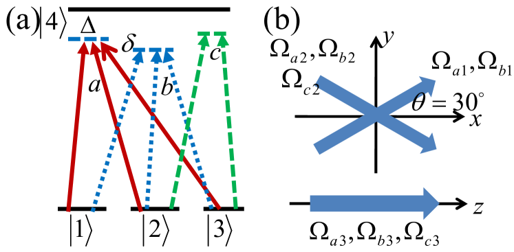
Figure 1: (Color online) Schematic representation of the light-atom interaction for the generation of the effective Hamiltonian (4). $a$, $b$, $c$ are three sets of lasers. Soild: $\Omega_{ai}$; Dotted: $\Omega_{bi}$; Dashed: $\Omega_{ci}$. $\Delta$ is the laser detuning of laser set $a$, $\delta$ is a small shift of the detuning for laser sets $b$ and $c$ from $\Delta$. (b) The configuration of the laser beams. All lasers are uniform plane waves.

The Rabi frequencies $\Omega_{ai}$ can be parameterized as $\Omega_{a1}=\Omega_{a}\sin\theta\cos\varphi e^{iS_{1}}$, $\Omega_{a2}=\Omega_{a}\sin\theta\sin\varphi e^{iS_{2}}$, $\Omega_{a3}=\Omega_{a}\cos\theta e^{iS_{3}}$, and $\Omega_{a}=\sqrt{\left|\Omega_{a1}^{2}\right|+\left|\Omega_{a2}^{2}\right|+\left|\Omega_{a3}^{2}\right|}$. The diagonalization of $H_{I}$ yields two degenerate dark states: $\left|D_{1}\right\rangle=\sin\varphi e^{iS_{31}}\left|1\right\rangle-\cos\varphi e^{iS_{32}}\left|2\right\rangle$, $\left|D_{2}\right\rangle=\cos\theta\cos\varphi e^{iS_{31}}\left|1\right\rangle+\cos\theta\sin\varphi e^{iS_{32}}\left|2\right\rangle-\sin\theta\left|3\right\rangle$, with $S_{ij}=S_{i}-S_{j}$. We choose a laser configuration illustrated in Fig. 1b with the parameters $\varphi=\pi/4$, $\theta=\arctan\sqrt{2}$, $S_{i}=\mathbf{q}_{i}\cdot\mathbf{R}$, $\mathbf{q}_{1}=q_{0}\left(\cos\frac{\pi}{6}\mathbf{e}_{x}+\sin\frac{\pi}{6}\mathbf{e}_{y}\right)$, $\mathbf{q}_{2}=q_{0}\left(\cos\frac{\pi}{6}\mathbf{e}_{x}-\sin\frac{\pi}{6}\mathbf{e}_{y}\right)$, $\mathbf{q}_{3}=q_{1}\mathbf{e}_{z}$, $\mathbf{R}=\left(x,y,z\right)$. The lasers $\Omega_{a1}$, $\Omega_{a2}$ are in the $xy$ plane, $\Omega_{a3}$ is along the $z$ direction, and $\left|\Omega_{a1}\right|=\left|\Omega_{a2}\right|=\left|\Omega_{a3}\right|$. Note that these three lasers are uniform plane waves, which are different from the optical lattices used in a previous scheme Zhang to generate RSOC. The effective low-energy Hamiltonian is obtained by projecting the Hamiltonian (1) onto the subspace of the degenerate dark states spanned by $\left|D_{i}\right\rangle$

$$H_{e}=\gamma k^{2}-\mu-\alpha\left(k_{x}\sigma_{z}+k_{y}\sigma_{x}\right)+V,$$ (2)

where $\gamma=\hbar^{2}/2m$, $\alpha=\gamma q_{0}/\sqrt{3}$, $V_{ij}=\left\langle D_{i}\right|V_{ext}\left|D_{j}\right\rangle$ is the effective external potential. The external harmonic trap $V_{trap}=V\left(\mathbf{r}\right)\sum\nolimits_{i=1}^{3}\left|i\right\rangle\left\langle i\right|$ is chosen to be spin-independent to avoid heating of atoms, where $V\left(\mathbf{r}\right)=m\omega_{t}^{2}r^{2}/2$, $\mathbf{r}=\left(x,y\right)$ is the coordinate in the $xy$ plane, $\omega_{t}$ is the trapping frequency.

Two additional laser sets $b$, $c$ with Rabi frequencies $\Omega_{bi}$, $\Omega_{ci}$ in Fig. 1 induce two Raman transitions between different hyperfine ground states, yielding an effective coupling interaction

$$H_{Z}=-\frac{\hbar}{\Delta}\left(\begin{array}[]{ccc}\left|\Omega_{b1}^{2}\right|&\Omega_{b1}^{\ast}\Omega_{b2}&\Omega_{b1}^{\ast}\Omega_{b3}\\ \Omega_{b2}^{\ast}\Omega_{b1}&\digamma_{1}&\digamma_{3}\\ \Omega_{b3}^{\ast}\Omega_{b1}&\digamma_{3}^{\ast}&\digamma_{2}\end{array}\right)$$ (3)

for atoms at the hyperfine ground states $\left|1\right\rangle$, $\left|2\right\rangle$, $\left|3\right\rangle$, where $\digamma_{1}=\left|\Omega_{b2}^{2}\right|+\left|\Omega_{c2}^{2}\right|$, $\digamma_{2}=\left|\Omega_{b3}^{2}\right|+\left|\Omega_{c3}^{2}\right|$, $\digamma_{3}=\Omega_{b2}^{\ast}\Omega_{b3}+\Omega_{c2}^{\ast}\Omega_{c3}$. We choose the detunings $\Delta_{b}$, $\Delta_{c}$ for the two sets ($b$ and $c$) of lasers as $\Delta_{b}=\Delta+\delta$, $\Delta_{c}=\Delta-\delta$, with $\delta\sim 2\pi\times 80$ MHz$\ll\Delta$. The small shifts of the detunings do not change the effective Rabi coupling between different hyperfine ground states, but remove the interference among different sets of lasers. The optical potentials generated by the laser sets $b$ and $c$ are taken as external potentials. With suitably chosen Rabi frequencies: $\Omega_{b1}=i\sqrt{3}\Omega_{0}e^{iS_{1}}$, $\Omega_{b2}=-\Omega_{0}e^{iS_{2}}$, $\Omega_{b3}=\Omega_{0}e^{iS_{3}},\Omega_{c2}=\sqrt{2}e^{i\pi/3}\Omega_{0}e^{iS_{2}}$, $\Omega_{c3}=\sqrt{2}\Omega_{0}e^{iS_{3}}$, the Hamiltonian (3) reduces to $H_{Z}=ih_{0}\left(\left|D_{2}\right\rangle\left\langle D_{1}\right|-\left|D_{1}\right\rangle\left\langle D_{2}\right|\right)$ with $h_{0}=3\hbar\Omega_{0}^{2}/\Delta$. Here $\Omega_{0}$ is the magnitude of the Rabi frequency of the laser $b2$. Within the dark state basis $\left|D_{i}\right\rangle$, $H_{Z}=h_{0}\sigma_{y}$. Under a new dark state basis $\left|\chi_{1}\right\rangle=\left(\left|D_{1}\right\rangle-i\left|D_{2}\right\rangle\right)/\sqrt{2}$, $\left|\chi_{2}\right\rangle=\left(-i\left|D_{1}\right\rangle+\left|D_{2}\right\rangle\right)/\sqrt{2}$, which corresponds to a unitary rotation of $\left|D_{i}\right\rangle$, the Hamiltonian (2) becomes

$$H_{e}=\gamma k^{2}-\mu+\alpha\left(k_{x}\sigma_{y}-k_{y}\sigma_{x}\right)+h_{0}\sigma_{z}+V\left(\mathbf{r}\right),$$ (4)

where the third term is the RSOC, the fourth term is the PZF. All eight lasers used for the generation of RSOC and PZF are uniform plane waves, therefore they do not lead to spatial periodic modulation of the atomic density. In addition, these lasers propagate only along three different directions (the same as other tripod schemes Ruseckas ; Ruseckas2 ; Clark1 ; Zhang ), therefore our scheme should be feasible in experiments.

Under the local density approximation with the local chemical potential $\mu\left(\mathbf{r}\right)=\mu-m\omega_{t}^{2}r^{2}/2$, the Hamiltonian (4) has two eigenenergies $\varepsilon_{\mathbf{k}\pm}=\gamma k^{2}-\mu\left(\mathbf{r}\right)\pm E_{0}$ with $E_{0}=\sqrt{h_{0}^{2}+\alpha^{2}k^{2}}$. There is an energy gap $E_{g}=2h_{0}$ opening between two spin orbit bands at $k=0$ (Fig. 2a). The intrinsic AHE is nonzero only when the chemical potential $\mu\left(\mathbf{r}\right)$ lies inside the gap.

The dynamics of cold fermi atoms are described by the semiclassical equations of motion Niu4

$$\mathbf{\dot{r}}=\partial\varepsilon_{\mathbf{k}}/\partial\mathbf{k}-\mathbf{\dot{k}\times\Gamma}_{z}\text{, }\mathbf{\dot{k}}=\mathbf{F/\hbar,}$$ (5)

where $\Gamma\left(\mathbf{k}\right)=\alpha^{2}h_{0}/2\left(\alpha^{2}k^{2}+h_{0}^{2}\right)^{3/2}\mathbf{e}_{z}$ is the Berry curvature in the momentum space and the physical origin of many topological phenomena. When there is a nonzero external force $\mathbf{F}$ along the $x$ direction, an anomalous velocity $\mathbf{v}_{AH}=-\mathbf{\dot{k}\times\Gamma}$ of atoms is induced along the $y$ direction. $\mathbf{v}_{AH}$ is the physical origin of the intrinsic AHE in electronic systems. However, it is difficult to perform a similar transport measurement commonly used for electronic systems for cold atoms in a harmonic trap. In the schemes for the observation of SHE in cold atoms Zhu ; Liu ; Liu2 , the time-of-flight image has been proposed. Because of the anomalous velocity $\mathbf{v}_{AH}$, we expect the time-of-flight expansion of cold atoms with RSOC, PZF and the gravitational force $\mathbf{F}=m\mathbf{g}$ (along the $x$ direction) has a transverse shift along the $y$ direction.

We assume that the harmonic trap in the $xy$ plane is suddenly turned off at $t=0$, and atoms start to expand, following the equations of motion (5). The column density along $y$ direction after the expansion depends on the initial atom distribution in both momentum and real spaces

$$n\left(y_{f},T,t\right)=\int d^{2}\mathbf{r}_{i}\int\frac{d^{2}\mathbf{k}}{\left(2\pi\right)^{2}}\delta\left(y_{f}-y_{i}-\Delta y\left(t\right)\right)f,$$ (6)

where $T$ is the temperature, $t$ is the time of flight. $\mathbf{r}_{i}$ ($y_{i}$) is the initial position of atoms, and $f\left(\mathbf{k},\mathbf{r}_{i},T\right)=1/\left(\exp\left[\left(\varepsilon_{\mathbf{k}}-\mu\left(\mathbf{r}_{i}\right)\right)/k_{B}T\right]+1\right)$ is the Fermi-Dirac distribution of atoms. $y_{f}$ is the position of atoms at time $t$. $\Delta y\left(t\right)=\int_{k_{x}}^{k_{x}+Ft/\hbar}dk_{x}^{\prime}\left(\frac{1}{F}\frac{\partial\varepsilon_{\mathbf{k}}}{\partial k_{y}}+\Gamma_{z}\left(k_{x}^{\prime},k_{y}\right)\right)$ is the distance of flight. $\delta\left(y\right)$ is the delta function.

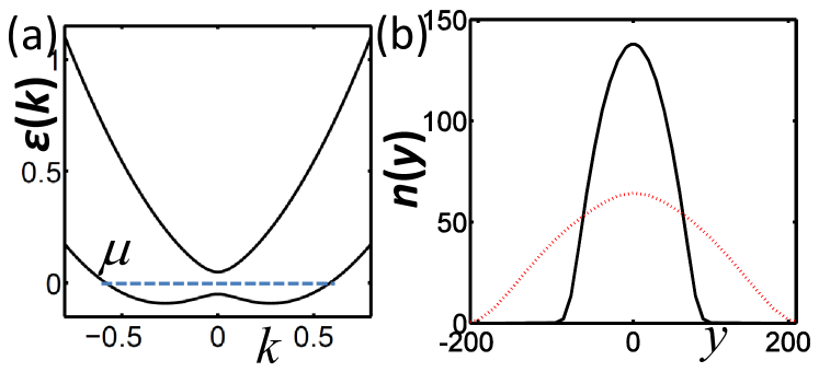
Figure 2: (Color online) (a) The spin-orbit band structure. $h_{0}=0.05E_{R}$. $\alpha^{2}/\gamma=1/3E_{R}$. We use the wavelength $\lambda=767$ nm of the ${}^{40}K$ D₂ transition line, the wavevector $k_{R}=2\pi/\lambda$, the recoil frequency $\omega_{R}=\hbar k_{R}^{2}/2m=2\pi\times 8.5KHz$, the recoil energy $E_{R}=\hbar\omega_{R}$, as the units of length, wavevector, frequency, and energy, respectively. $E_{R}$ corresponds to a temperature $T=2\mu K$. (b) The time of flight image of atoms in the presence of PSOC, PZF, and gravitational force. The unit of the density is $k_{R}^{2}=6.7\times 10^{9}$ cm^-2. $\mu=0$, $T=20nK$, $\omega_{t}=2\pi\times 10Hz$. Solid: $t=0$; Dotted: $t=19$ ms.

In Fig. 2b, we plot the column density $n\left(y_{f},T,t\right)$ at two different times. At $t=0$, the initial column density is symmetric along the $y$ axis. After a time $t$, $n\left(y_{f},T,t\right)$ becomes asymmetric because of the anomalous velocity of atoms. However, the expansion dynamics of atoms is dominated by the first term in $\Delta y\left(t\right)$, and the differences of the atomic densities at $\pm y_{f}$ correspond to only a small percentage (below 3%) of the total density. Therefore it may be hard to observe them in experiments. The difference between electrons and cold atoms comes from the fact that $\partial\varepsilon_{\mathbf{k}}/\partial k_{y}$ in an electronic system does not contribute to the overall transverse motion (the observed Hall current is purely from the anomalous velocity), while the initial atom velocities $\partial\varepsilon_{\mathbf{k}}/\partial k_{y}$ dominate the expansion process and the asymmetry of the column density should be small in an atomic system. Therefore we need develop other techniques for the observation of the intrinsic AHE.

Recently, the response of atomic density to a rotation of the trap has been proposed for measuring quantum Hall conductivity for cold atoms based on the well-known Strĕda formula Streda $\sigma=\partial n/\partial B$. Here the rotation for atoms is equivalent to the magnetic field for electrons. However, the Strĕda formula does not apply to the AHE because it is not quantized. Nevertheless, the density response to the rotation still contains rich information about the intrinsic AHE. Consider a rotation of the harmonic trap along the $z$ axis Haljan , the Hamiltonian can be written as

$$H = \hbar^{2}q^{2}/2m+\alpha\left(q_{x}\sigma_{y}-q_{y}\sigma_{x}\right)$$ (7)

$$+h_{0}\sigma_{z}+m\left(\omega_{t}^{2}-\varpi^{2}\right)r^{2}/2-\mu$$

in the rotation frame, where $\hbar\mathbf{q}=\hbar\mathbf{k}-m\varpi\mathbf{\hat{z}}\times\mathbf{r}$ is the mechanical momentum of atoms Niu4 , $\varpi$ is the rotation frequency of the trap. The density of atoms is

$$n\left(\mathbf{r}\right)=\left(2\pi\right)^{-2}\int d^{2}\mathbf{q}\left[1+m\varpi\Gamma_{z}/\hbar\right]f\left(\mathbf{q},\mathbf{r,}\varpi\right),$$ (8)

where $m\varpi\Gamma_{z}/\hbar$ is a correction to the well-known constant density of states $1/\left(2\pi\right)^{2}$ in the presence of nonzero Berry curvature fields and the rotation Xiao . $f\left(\mathbf{q},\mathbf{r,}\varpi\right)=1/\left(\exp\left[\left(\varepsilon_{\mathbf{m}}-\mu\left(\mathbf{r}\right)\right)/k_{B}T\right]+1\right)$ is the Fermi Dirac distribution of atoms, where the energy of atoms $\varepsilon_{\mathbf{m}}=\varepsilon_{\mathbf{q}}-M_{z}\varpi$ contains a correction $-M_{z}\varpi=-m\varpi\alpha^{2}h_{0}/4\hbar\left(\alpha^{2}q^{2}+h_{0}^{2}\right)$, known as the magnetization energy for electrons in the solid state Niu4 .

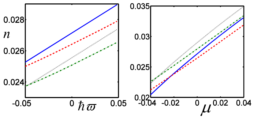
Figure 3: (Color online) Plot of the atom density $n\left(\varpi,\mu,T\right)$ with respect to $\hbar\varpi$ and $\mu$. The units are the same as that in Fig. 2. $h_{0}=0.05E_{R}$. $\alpha^{2}/\gamma=1/3E_{R}$. Solid and dotted: $T=2nK$; Dashed and dash dotted: $T=200nK$. (a) Solid and dashed: $\mu=0$; Dotted and dash dotted: $\mu=-0.01E_{R}$. (b) Solid and dashed: $\varpi=0$; Dotted and dash dotted: $\varpi=0.05\omega_{R}$.

We assume the rotation frequency $\varpi$ of the trap is slowly increased to keep the same temperature of the system. The local chemical potential can be fixed by increasing $\omega_{t}$ with $\varpi$. The response of the atom density to $\varpi$ is

$$\frac{\partial n}{\partial\varpi}=\int\frac{d^{2}\mathbf{q}}{\left(2\pi\right)^{2}}\left[\frac{m}{\hbar}\Gamma_{z}f+\left(1+\frac{m\varpi\Gamma_{z}}{\hbar}\right)\frac{\partial f}{\partial\mu}M_{z}\right]$$ (9)

for fixed $\mu$ and $T$. At $T=0$ and $\varpi=0$, Eq. (9) reduces to

$$\frac{\partial n}{\partial\varpi}=\frac{m}{\hbar}\int^{\mu}\frac{d^{2}\mathbf{q}}{\left(2\pi\right)^{2}}\Gamma_{z}\mathbf{+}\frac{M_{z}}{4\pi}\frac{1}{d\varepsilon_{\mathbf{q}}/dq^{2}|_{\varepsilon_{\mathbf{q}}=\mu}}.$$ (10)

Here the first term is the anomalous Hall conductivity $\sigma_{xy}$ for cold atoms. In the parameter region $\left|\mu\left(r\right)\right|<h_{0}$ (i.e., the chemical potential lies in the band gap), it yields $\sigma_{xy}=m\left[1-h_{0}/\sqrt{\alpha^{2}q_{F}^{2}\left(r\right)+h_{0}^{2}}\right]/4\pi\hbar$, where the Fermi wavevector $q_{F}\left(r\right)$ is obtained from $\varepsilon_{\mathbf{q}_{F}}=\mu\left(r\right)$. In the parameter region $\alpha^{2}/\gamma\gg h_{0}$, $q_{F}^{2}\approx\alpha^{2}/\gamma^{2}$ and $\sigma_{xy}\approx m/4\pi\hbar$. The second term $\bar{\sigma}_{xy}$, originating from the non-zero orbit magnetic moment $M_{z}$, is an additional contribution to $\partial n/\partial\varpi$ that was missing in the previous literature Xiao for electron systems. Eq. (10) is a generalization of Strĕda formula for the anomalous Hall effects. By varying parameters and measuring the density response, we can extract information not only about the anomalous Hall conductivity, but also the magnetic moment that is generally hard to measure in solid state systems. In the parameter region $\alpha^{2}/\gamma\gg h_{0}$, $\bar{\sigma}_{xy}\approx\gamma mh_{0}/8\pi\hbar\alpha^{2}\ll m/4\pi\hbar\approx\sigma_{xy}$. Therefore $\sigma_{xy}$ dominates in Eq. (9) in this region, and the density response $\partial n/\partial\varpi$ yields a rough measurement for the anomalous Hall conductivity.

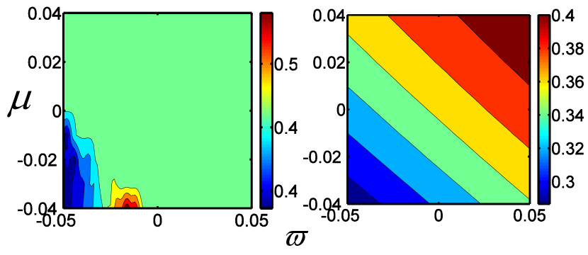
Figure 4: (Color online) Plot of $\partial n\left(\varpi,\mu,T\right)/\partial\varpi$ with respect to $\varpi$ and $\mu$. The unit of $\partial n\left(\varpi,\mu,T\right)/\partial\varpi$ is taken to be $m/2\pi\hbar$. The other units are the same as that in Fig. 2. $h_{0}=0.05E_{R}$ and $\alpha^{2}/\gamma=E_{R}/3$. (a) $T=2$ nK (b) $T=200$ nK.

We numerically calculate the density $n$ and density response $\partial n/\partial\varpi$ as functions of the parameters $\left(\mu,\varpi,T\right)$, and plot them in Figs. 3 and 4 for $T=200$ nK and 2 nK. The presence of the harmonic trap changes the chemical potential at $r$ by $-m\left(\omega_{t}^{2}-\varpi^{2}\right)r^{2}/2$. In a realistic experiment, the effective trapping frequency $\sqrt{\omega_{t}^{2}-\varpi^{2}}$ in the presence of rotation may be slightly different from the initial trapping frequency $\omega_{t0}$ without rotation to keep the same temperature of the system Ho . This can be overcome by comparing the densities at different spatial points $r$, $r^{\ast}$ such that $\mu-\frac{1}{2}m\left(\omega_{t}^{2}-\varpi^{2}\right)r^{\ast 2}=\mu-\frac{1}{2}m\omega_{t0}^{2}r^{2}$ to keep the same local chemical potential Ho . With this method, we can measure the density response to the rotation with the fixed temperature and chemical potential. In addition, the rotation of the system requires an asymmetric harmonic trap Haljan , which does not affect our results because it only change the spatial positions for the measurement of the density change at a fixed chemical potential through a different local chemical potential dependence $\mu\left(\mathbf{r}\right)=\mu-m[\left(\omega_{tx}^{2}-\varpi^{2}\right)x^{2}+\left(\omega_{ty}^{2}-\varpi^{2}\right)y^{2}]/2$. We adopt a set of parameters: $\alpha^{2}/\gamma=E_{R}/3=2\pi\hbar\times 2.8$ KHz, $h_{0}=2\pi\hbar\times 425$ Hz, $\omega_{t0}=2\pi\times 50$ Hz, $\varpi_{\max}=0.05\omega_{R}=2\pi\times 425Hz$, $\omega_{t}\approx\sqrt{\omega_{t0}^{2}+\varpi^{2}}$, $\omega_{t}-\varpi=\omega_{t0}^{2}/\left(\omega_{t}+\varpi\right)\approx 2\pi\times 3Hz$. At $r=0.1\lambda\omega_{R}/\pi\omega_{t0}$ $=4.2\mu m$, the chemical potential $\mu$ changes by $0.01E_{R}$. From Figs. 3 and 4, we see a maximum density change at the order of $3\times 10^{7}$ cm^-2 can be observed with a rotation frequency $\varpi_{\max}$, which corresponds to about 10% of the total density and can be observed in a realistic experiment. The density variation at a medium temperature $T=200$ nK is at the same order as that at a low temperature $T=2$ nK. Note that the multiple layer structure induced by the optical lattice confinement along the $z$ direction can further enhance the signal.

In summary, we propose a scheme to create RSOC and PZF simultaneously for cold atomic gases. We show that, by measuring the atomic density response to a rotation of the trap, the intrinsic AHE can be observed for cold fermionic atoms in a harmonic trap. We emphasize that the creation of RSOC and PZF brings new opportunities for studying many topological phenomena, such as chiral p-wave superfluids, anomalous and spin Hall insulators, etc.

Acknowledgments: We thank Di Xiao and Qian Niu for helpful discussion. This work is supported by the ARO (W911NF-09-1-0248) and DARPA-YFA (N66001-10-1-4025).

References

• (1) I. ZutiΔ‡, J. Fabian, and S. Das Sarma, Rev. Mod. Phys. 76, 323 (2004).
• (2) T. Jungwirth, Q. Niu, and A. H. MacDonald, Phys. Rev. Lett. 88, 207208 (2002).
• (3) J. Sinova et al., Phys. Rev. Lett. 92, 126603 (2004).
• (4) N. Nagaosa et al., Rev. Mod. Phys. 82, 1539 (2010).
• (5) B. T. Seaman et al., Phys. Rev. A 75, 023615 (2007).
• (6) J. Ruseckaset al., Phys. Rev. Lett. 95, 010404 (2005).
• (7) S.-L. Zhu et al., Phys. Rev. Lett. 97, 240401 (2006).
• (8) X.-J. Liu et al., Phys. Rev. Lett. 98, 026602 (2007).
• (9) X.-J. Liu et al., Phys. Rev. Lett. 102, 046402 (2009).
• (10) G. Juzeliunas et al., Phys. Rev. Lett. 100, 200405 (2008).
• (11) J. Y. Vaishnav et al., Phys. Rev. Lett. 101, 265302 (2008).
• (12) J. Y. Vaishnav and C. W. Clark, Phys. Rev. Lett. 100, 153002 (2008).
• (13) T. D. Stanescu, C. Zhang, and V. Galitski, Phys. Rev. Lett. 99, 110403 (2007).
• (14) C. Zhang et al., Phys. Rev. Lett. 101, 160401 (2008).
• (15) J. D. Sau, et al., Phys. Rev. Lett. 104, 040502 (2010).
• (16) C Nayak et al., Rev. Mod. Phys. 80, 1083 (2008).
• (17) P. StrΔ•da, J. Phys. C 15, L717 (1982).
• (18) R. O. Umucalilar, Hui Zhai, M. O. Oktel, Phys. Rev. Lett. 100, 070402 (2008).
• (19) D. Xiao, J. Shi, and Q. Niu, Phys. Rev. Lett. 95, 137204 (2005).
• (20) G. Sundaram, and Q. Niu, Phys. Rev. B, 59, 14915 (1999).
• (21) P. C. Haljan et al., Phys. Rev. Lett. 87, 210403 (2001).
• (22) T.-L. Ho, and Q. Zhou, Nat. Phys. 6, 131 (2010).