Fluctuation Domains in Adaptive Evolution

Abstract

We derive an expression for the variation between parallel trajectories in phenotypic evolution, extending the well known result that predicts the mean evolutionary path in adaptive dynamics or quantitative genetics. We show how this expression gives rise to the notion of fluctuation domains – parts of the fitness landscape where the rate of evolution is very predictable (due to fluctuation dissipation) and parts where it is highly variable (due to fluctuation enhancement).  These fluctuation domains are determined by the curvature of the fitness landscape.  Regions of the fitness landscape with positive curvature, such as adaptive valleys or branching points, experience enhancement. Regions with negative curvature, such as adaptive peaks, experience dissipation.  We explore these dynamics in the ecological scenarios of implicit and explicit competition for a limiting resource.

1 Introduction

Fitness landscapes have long been an important metaphor in evolution. Wright (1931) originally introduced the concept to explain his result that the mean rate of evolution of a quantitative trait is proportional to gradient of its fitness.  The result and its accompanying metaphor continue to arise in evolutionary theory, having been derived independently in quantitative genetics (Lande, 1979), game-theoretic dynamics (Hofbauer and Sigmund, 1998; Abrams, 1993), and adaptive dynamics (Dieckmann and Law, 1996).  The metaphor creates a deterministic image of evolution as the slow and steady process of hill climbing.  Other descriptions of evolution have focused on its more stochastic elements – the random chance events of mutations and the drift of births and deaths that underlie the process (Kimura, 1984, 1968; Ohta, 2002).  In this manuscript, we seek to characterize the deviations or fluctuations of evolutionary trajectories around the expected evolutionary path.

Our main result is that the size of deviations of evolutionary trajectories is determined largely by the curvature of the evolutionary landscape whose gradient is determining the mean rate of evolution. The landscape metaphor can be used to understand the interplay of stochastic and deterministic forces by identifying regimes where the selection will counterbalance or enhance such stochastic fluctuations. Because curvature can be positive (concave up) or negative (concave down), the evolutionary landscape can be divided into domains where fluctuations are enhanced or dissipated.  To make this more precise, we focus on a Markov model of evolution used in the theory of adaptive dynamics.  This Markov model gives rise to the familiar gradient equation – like that which first inspired the fitness landscapes metaphor – and also a more precise statement of the fluctuation dynamics.  The adaptive dynamics framework is general enough that we can consider how these results apply in a variety of ecological scenarios. We illustrate the surprising consequence of bimodal distributions of expected phenotypes among parallel trajectories emerging from a fixed starting point on a single-peak adaptive landscape due to fluctuation enhancement. We also provide a landscape interpretation that suggests how the ideas of fluctuation dynamics apply to other ecological and evolutionary models.

2 Theoretical construction

Various definitions of fitness landscape have been used in the study of evolutionary dynamics. The conventional idea postulates a mapping between trait values and fitness (Levins, 1962, 1964; Rueffler et al., 2004).  The difficulty with this conception is that, in many cases, fitness of a given population type is mediated largely through competition with other populations, and is thus dependent on the current distribution of populations and their respective phenotypes in the environment. This dependence on densities or frequencies turns the static fitness landscape into a dynamic landscape, whose shape changes as the number of individuals, and their corresponding traits, changes.

It is possible to depict the fitness landscape that emerges even in the face of density- or frequency-dependent competition by returning to Wright’s notion of a landscape. To do so, consider a resident population of individuals in an environment, each of which have an identical trait value, i.e., a monomorphic population. Next, consider the per-capita fitness of a small number of mutant individuals with a similar, but different trait.  The per-capita fitness of mutants in the environment may be larger, smaller or identical to the per-capita fitness of residents. The gradient in fitness around the trait represented by the resident is termed the selective derivative (Geritz et al., 1997) in adaptive dynamics (analogous to the selective gradient in quantitative genetics). The fitness landscape is defined by integrating over these derivatives in trait space, to obtain a local picture of how fitness changes.  In the limit of small, slow mutation, it can be shown that the population will evolve as predicted by the shape of the landscape: by climbing towards a peak most rapidly when the slope is steep (Rueffler et al., 2004), see Fig. 1 for three illustrative examples.   The trait on the horizontal axis is that of the resident, not the mutant.  The lower panels show the slope of the mutant fitness as a function of the resident trait (up to a multiplicative factor)– the slope of the mutant fitness changes as the resident trait changes. The trait of the resident population evolves in the direction given by that slope.  Integrating the lower panel along the resident trait axis reveals the fitness landscape the resident trait climbs in an evolutionary process (top panels). Note that changes in the mutant fitness are captured in the changes in slope of the landscape; the fitness landscape itself remains fixed. We derive the expected evolutionary dynamics of the phenotypic trait of the resident and its variation among parallel trajectories in the following sections.

2.1 Model

Consider a population monomorphic for a particular phenotypic trait, $x$.  The abundance of the population, $N(x,t)$ of trait $x$, is governed by its ecological dynamics:

$$\frac{\mathrm{d}N(x)}{\mathrm{d}t}=f(x,N,E),$$ (1)

which may depend on the trait, population abundance, and the environmental conditions, $E$.  The evolutionary dynamics proceed in three steps  (Dieckmann and Law, 1996; Champagnat et al., 2006).  First, the population assumes its equilibrium-level abundance $N^{\ast}(x)$, determined by its phenotypic trait $x$.  Next, mutants occur in the population at a rate given by the individual mutation rate $\mu$ times the rate of births at equilibrium, $b(x)$.  The mutant phenotype, $y$, is determined by a mutational kernel, $M(x,y)$. The success of the mutant strategy depends on the invasion fitness, $s(y,x)$, defined as the per-capita growth rate of a rare population. Mutants with negative invasion fitness die off, while mutants with positive invasion fitness will invade with a probability that depends on this fitness (Geritz et al., 1997).

The invasion fitness is calculated from the ecological dynamics, Eq. (1), and will in general depend on the trait $x$ of the resident population as well as that of the mutant, $y$.  We assume that a successful invasion results in replacement of the resident (Geritz et al., 1997, 2002), and the population becomes monomorphically type $y$.  The details of this formulation can be found in Appendix A.  The important observation is that such a model can be represented by a Markov process on the space of possible traits, $x$.  The population can jump from any position $x$ to any other position $y$ at a transition rate $w(y|x)$ determined solely by the trait values $x$ and $y$.  The probability that the process is at state $x$ at time $t$ then obeys the master equation for the Markov process,

$$\frac{\mathrm{d}}{\mathrm{d}t}P(x,t)=\int\mathrm{d}y\  \left[w(x|y)P(y,t)-w(y|x)P(x,t)\right].$$ (2)

No general solution to the master equation (2) exists. However, if the jumps from state $x$ to state $y$ are sufficiently small (i.e., if mutants are always close to the resident), we can obtain approximate solutions for $P(x,t)$ by applying a method known as the Linear Noise Approximation (van Kampen, 2001), Appendix B.  Doing so yields a general solution for the probability $P(x,t)$ in terms of the transition rates, $w(y|x)$, Eq. (23).  The linear noise approximation derives a diffusion equation as an approximation to the original jump process, as is commonly postulated.  While this diffusion can be written as a partial differential equation (PDE), following Kimura, or as a stochastic differential equation, the solution for the probability density can be proven to be Gaussian and hence it suffices to write down ordinary differential equations for the first two moments (Kurtz, 1971).

2.2 The Fluctuation Equation

We assume the mutational kernel $M(y,x)$ is Gaussian in the difference between resident and mutant traits, $y-x$, with width $\sigma_{\mu}$ and that mutations occur at rate $\mu$. A more thorough discussion of these quantities can be found in Appendix A, where they are developed in the process of deriving the transition probability $w(y|x)$ that specifies the underlying Markov process. Using Eq. (23) which results from the systematic expansion of the master equation (2), the mean trait $\hat{x}$ obeys

$$\frac{\mathrm{d}\hat{x}}{\mathrm{d}t}=\frac{1}{2}\mu\sigma_{\mu}^{2}N^{*}(\hat{x})\partial_{y}s(y,\hat{x})|_{y=\hat{x}}\equiv a_{1}(\hat{x}),$$ (3)

with an expected variance $\sigma^{2}$ that obeys

$$\frac{\partial\sigma^{2}}{\partial t}=2\sigma^{2}\partial_{\hat{x}}a_{1}(\hat{x})+2\sqrt{\tfrac{2}{\pi}}\sigma_{\mu}\left|a_{1}(\hat{x})\right|.$$ (4)

Eq. (3) recovers the familiar canonical equation of adaptive dynamics (Dieckmann and Law, 1996) for the mean trait. Eq. (4), which describes the variance, we term the fluctuation equation of adaptive dynamics. The linear noise approximation (see Appendix B) also predicts that the probability distribution itself is Gaussian, so that Eqs. (3) and (4) determine the entire distribution of possible trajectories in this approximation. To illustrate the local behavior of the model, we define the fitness landscape as $L(x)=\int_{0}^{x}a_{1}(y)\,dy$.

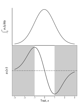
(a) Implicit Resource

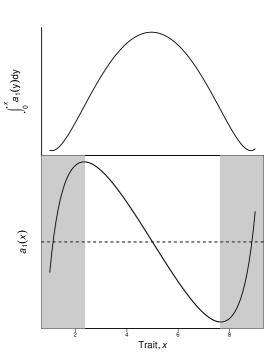
(b) Chemostat

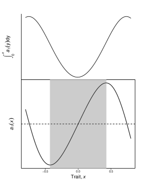
(c) Branching

Figure 1: Fluctuation domains. The lower panels show the rate of evolution given by Eq. (3) vs. the resident trait $x$ for three ecological models: (a) implicit competition for a limiting resource (Section 4), (b) explicit resource competition (Appendix C), and (c) symmetric branching for dimorphic populations (with a resident population of trait $x$ and another at $-x$, Appendix E). The horizontal dashed lines in the lower panel denote where $a_{1}(x)=0$, i.e., the selective derivative is zero, and correspond to evolutionarily singular points, e.g., adaptive peaks and valleys. Shaded and unshaded regions in the lower panels correspond to trait values for which fluctuations are enhanced (shaded) and dissipated (unshaded). The adaptive landscape is defined as the integral of this expression (upper panels) – where populations climb the hills at a rate proportional to their steepness. Note that the adaptive landscape for the symmetric branching case has two peaks, and so evolutionary trajectories will lead to a stable dimorphism.

3 Fluctuation Domains

A closer look at Eq. (4) will help motivate our geometric interpretation of fluctuation domains. The approximation requires that the mutational step size $\sigma_{\mu}$ is very small, hence the second term will almost always be much smaller than the first (except when the fluctuations $\sigma$ themselves are also very small). Note that the second term resembles the right-hand side of (3), differing only by a small scalar constant and the fact that it is always positive. Interestingly, this means that the second term vanishes at the singular point where $a_{1}(\hat{x})=0$ and $\sigma^{2}=0$: fluctuations cannot be introduced at an evolutionary equilibrium. That the first term is the gradient of the deterministic (mean) dynamics and the second term is smaller by a factor of the small parameter in the expansion are general features of the linear noise approximation.

The first term of (4) implies that the variance $\sigma^{2}$ will increase or decrease exponentially at a rate determined by $\partial_{x}a_{1}(x)$; i.e., the curvature of the fitness landscape. This landscape and its gradient are depicted in Fig. 1 for several ecological scenarios. Plotting the gradient itself makes it easier to see when fluctuations will increase or decrease. On the gradient plot the singular point is found where the curve crosses the horizontal axis.

In the neighborhood of a singular point corresponding to an adaptive peak, the slope is negative, hence the first term in Eq. (4) (the coefficient of $\sigma^{2}$) is negative and fluctuations dissipate exponentially. This means that two populations starting with nearby trait values will converge to the same trajectory. In this region no path will stochastically drift far from the mean trajectory, hence the canonical equation will provide a good approximation of all observed paths. We term the part of the trait-space landscape where $\partial_{x}a_{1}(x)<0$ the fluctuation-dissipation domain, analogous to the fluctuation-dissipation theorem found in other contexts (van Kampen, 2001).

Farther from the singular point corresponding to an adaptive peak, $\partial_{x}a_{1}(x)$ becomes positive (see Fig. 1(a) and Fig. 1(b)). While this part of trait-space still falls within the basin of attraction of the singular point, the variance $\sigma^{2}$ between evolutionary paths will grow exponentially. Initially identical populations starting with trait values in this region will experience divergent trajectories due to this enhancement. The variation can become quite large, with evolutionary trajectories that differ significantly from the mean. We call this region of trait-space where $\partial_{x}a_{1}(x)>0$ the fluctuation enhancement domain. Eventually trajectories starting in this region will be carried into the fluctuation-dissipation domain, where they will once again converge.

Evolutionary branching points (Dieckmann and Doebeli, 1999; Geritz et al., 1998) provide another example of a fluctuation enhancement domain. Until now, we have assumed that successful mutants replace the resident population, a result known as “invasion implies substitution” (Geritz et al., 2002). However, at an evolutionary branching point, the mutant invader no longer replaces the resident population, and the population becomes dimorphic. In dealing with monomorphic populations, we have been able to describe the evolutionary dynamics in terms of the change of a single trait, describing a single resident population. For dimorphic populations, two resident populations coexist, and both influence the shape of the landscape. Thus, an invader’s fitness, $s(y;x_{1},x_{2})$, and its rate of evolution, $a_{1}(x_{1},x_{2})$, will depend on how it performs against both populations. The evolutionary dynamics after branching are two-dimensional and require a multivariate version of Eq. (4). Despite this, we can still gain qualitative insight using the intuition that connects fluctuation domains to curvature.

The existence of the stable dimorphism fundamentally distorts the landscape. While the population was monomorphic, being closer to the singular point always ensured a higher fitness. Once a resident population sits on either side of a branching point though, the singular point becomes a fitness minimum. This description of evolution towards points which become fitness minima after branching has been addressed extensively elsewhere (Geritz et al., 1997, 1998; Geritz, 2004). Here, what interests us is the effect of branching on fluctuations. If the landscape is smooth, a minimum must have positive curvature and therefore must be an enhancement domain. The farther a mutant gets from the branching point, the faster it can continue to move away, thus enhancing the initially small differences between mutational jumps. A rigorous description of this effect would require a multivariate version of Eq. (4) which is beyond the scope of this paper. Instead, we illustrate the enhancement effect by taking a slice of the two-dimensional landscape by assuming that the dimorphic populations have symmetric trait values about the singular strategy, $x_{1}=-x_{2}=x$. The fitness landscape for the case of symmetric branching is shown in Fig 1(c), and the derivation provided in Appendix D. Note that the region around the branching point is a fluctuation enhancement regime and the two new fitness maxima far from the branching point are in fluctuation dissipation regimes.

To provide a more concrete illustration of the fluctuation dynamics, we will focus on the description of the ecological competition model and compare the theoretical predictions of Eq. (3) and Eq. (4) to point-process simulations of the Markov process (Gillespie, 1977).

4 An Example of Fluctuation Domains in Resource Competition

4.1 An Ecological Model of Implicit Competition for a Limiting Resource

The logistic model of growth and competition in which populations compete for a limited resource is a standard model in ecological dynamics (Dieckmann and Doebeli, 1999). Here, we consider the population dynamics of $N(x,t)$ individuals each with trait $x$:

$$\frac{\mathrm{d}N(x,t)}{\mathrm{d}t}=rN(x,t)\left(1-\frac{\sum_{y}N(y,t)C(x,y)}{K(x)}\right),$$ (5)

where $r$ is the birth rate and $\sum_{y}rN(y)C(x,y)/K(x)$ is the density-dependent death rate. In the model, $K(x)$ is the equilibrium population density and $C(x,y)$ is a function which describes the relative change in death rate of individuals of type $x$ due to competition by individuals of type $y$. Given $C(x,x)=1$, the equilibrium density of a monomorphic population is $N^{\ast}(x)=K(x)$. Following Dieckmann and Doebeli (1999) we assume the following Gaussian forms,

$$K(x)=K_{0}e^{-x^{2}/(2\sigma_{k}^{2})},$$ (6)

and

$$C(x,y)=e^{-(x-y)^{2}/(2\sigma_{c}^{2})},$$ (7)

where $\sigma_{k}$ and $\sigma_{c}$ are scale factors for the resource distribution and competition kernels respectively. We focus on the case $\sigma_{c}>\sigma_{k}$, for which the model has a convergence-stable evolutionarily stable strategy (ESS) at $x=0$ (Geritz et al., 1998). Having specified the ecological dynamics, we must also specify the evolutionary dynamics, which we assume occur on a much slower time scale. We assume that with probability $\mu$ an individual birth results in a mutant offspring, and that the mutant trait is chosen from a Gaussian distribution centered at the trait value of the parents and with a variance $\sigma_{\mu}^{2}$. From this we can assemble $w(y|x)$, and compute equations (3) and (4) (see Appendix B).

4.2 Numerical simulation of stochastic evolutionary trajectories

There are many ways to represent evolutionary ecology models in numerical simulations, including finite simulations, fast-slow dynamics, and point processes (Dieckmann and Doebeli, 1999; Nowak and Sigmund, 2004; Champagnat et al., 2006; Champagnat and Lambert, 2007). We choose to model the evolutionary trajectories of the ecological model in Eq. (5) by explicitly assuming a separation of ecological and evolutionary time scales. First, given a trait $x$, the ecological equilibrium density $N^{\ast}(x)$ is determined. Then, the time of the next mutant introduction is calculated based on a Poisson arrival rate of $\mu rN^{\ast}(x)$. In essence, we are assuming that ecological dynamics occur instantaneously when compared to evolutionary dynamics. The trait of the mutant, $y$, is equal to $x$ plus a normal deviate with variance $\sigma_{\mu}^{2}$. The mutant replaces the resident with probability given by the standard branching process result, $1-d(y,x)/b(y,x)$ where $d$ and $b$ are the per-capita birth and death rate of the mutant, respectively, so long as $b>d$, and with probability 0 otherwise. The ecological steady state is recalculated and the process continues. Simulations are done using Gillespie’s minimal process method (Gillespie, 1977). Estimates of the mean phenotypic trait $\hat{x}$ and the variance $\sigma^{2}$ are calculated from ensemble averages of at least $10^{5}$ replicates.

Figure 2: Simulations over fluctuation domains. The dynamics of the mean path, variance between paths, and snapshots of the trait distribution in time for three initial conditions: $x_{0}=1$, $x_{0}=2$, and $x_{0}=3$ (top to bottom successively). The three rows correspond to trajectories experiencing fluctuation dissipation (tow) and fluctuation enhancement (bottom) along with an intermediate case (middle). The mean (first column) and variance (second column) among trait values are plotted over time. Circles are simulation averages from $10^{5}$ replicates and lines are theoretical predictions. The final column shows the theoretical Gaussian distribution (solid line) at the point in time indicated by the dashed line and closed circle in the first two columns, and the actual histogram (circles) of positions across the replicates at that time. The bottom right panel shows a bimodal distribution among replicates in the case of fluctuation enhancement. Parameters: $\sigma_{k}^{2}=1$, $\sigma_{c}^{2}=1.01$, $r=10$, $\sigma_{\mu}=0.0005$, $\mu=1$.

4.3 Comparison of Theory and Simulation

We consider simulations with three different initial conditions: starting within the fluctuation-dissipation domain ($x=1)$, just into the fluctuation-enhancement domain ($x=2$), and deep into the fluctuation enhancement regime ($x=3)$ in successive rows in Fig. 2. For each condition, the simulation is repeated $10^{5}$ times and we compare the resulting distribution of trajectories to that predicted by theory. In the first column we plot the numerically calculated mean path taken to the ESS (shown in circles), and compare to the theoretical prediction of Eq. (3). In the second column, we plot the variance between paths, and compare to the predictions of Eq. (4). As each replicate begins under identical conditions, the initial variance is always zero. In the third column, we present the distribution of traits among the replicates at a single instant in time. We chose the moment of maximum variance so that deviations from the theoretically predicted Gaussian kernel will be most evident.

4.3.1 Fluctuation-Dissipation Domain

Starting at the edge of the dissipation domain, fluctuations grow for only a short time before rapidly decaying, in the first row of Fig. 2. Since the simulation is sampled at regular time intervals, the vertical spacing of points indicate the rate of evolution. Theoretical predictions closely match simulation results for both the mean and variance, and the resulting distribution matches the theoretically predicted Gaussian. The variance represents an almost negligible deviation from the mean trajectory.

4.3.2 Fluctuation-Enhancement Domain

Our second ensemble at $x=2$ begins clearly within the fluctuation-enhancement domain. In the second row of Fig. 2, the variance plot (center panel) begins by growing exponentially. Once the population crosses into the dissipation domain, at $x=1$, at about $t=1000$, the variance peaks and then dissipates exponentially. This transition appears as an inflection point in the mean path (left panel). Though the variation now represents significant deviations, the distribution still appears Gaussian (right panel).

4.3.3 Strong Fluctuations

In the third row of Fig. 2, starting deep within the fluctuation-enhancement domain at $x=3$, theory and simulation agree initially. Remaining long enough in this domain, fluctuations are eventually on the same order of magnitude as the macroscopic dynamics themselves, and the linear noise approximation underlying the theory begins to break down. The theory and simulation variance diverge, while the mean path is substantially slower than predicted by the canonical equation. In the right panel, the reason for this becomes clear. At this point in the divergence, the distribution is far from Gaussian, rather it has become bimodal, with some replicates having reached the stable strategy at $x=0$ and others having hardly left the initial state.

The mechanism behind the emergence of bimdal probability distributions for trajectories can be seen in the final row of Fig. 2. The theoretical trajectory predicted by Eq. (3) is sigmoidal, comprised of slow change at the beginning and end and rapid evolution in the middle. Ecologically, this arises at the beginning from the small population size available to generate mutations, and at the end from the weakening selection gradient. Populations with intermediate trait values hence experience rapid trait evolution, giving rise to this transiently bimodal distribution. The theory provides insight into this case of strong fluctuations in two ways – first, it is driven by the existence of a fluctuation-enhancement domain, and second, it is anticipated by the theoretical prediction of fluctuations that are on the same order as the macroscopic dynamics. We observe that these macroscopic fluctuations can arise whenever the population remains long enough in the enhancement regime, independent of other model details. The fluctuation equation for the explicit resource competition (chemostat) model shown in Fig. 1(b) and described in Appendix C never predicts fluctuations that reach macroscopic values, and simulations of this system (not shown) do not produce bimodal trait distributions.

5 Discussion

The metaphor of fitness landscapes has been a powerful tool for understanding evolutionary processes (Wright, 1932; Lande, 1979; Abrams, 1993; Dieckmann and Law, 1996). The concept of a landscape arises naturally from describing the rate of change of the mean trait as being proportional to the evolutionary gradient. We extend this metaphor to understand fluctuations away from this mean, where our analysis of a Markov process representation of evolution in the adaptive dynamics framework brings us back to the notion of a fitness landscape. In this case, it is the curvature of that landscape which informs the dynamics of these fluctuations away from the expected evolutionary path. Our result linking landscape curvature to fluctuation domains is consistent with similar results from quantitative genetics that relate the sign and magnitude of the quadratic selection coefficient in the Price equation to increases or decreases in trait variation (Lande and Arnold, 1983; Chevin and Hospital, 2008).

Though the mathematical analysis of the Markov process is somewhat technical, the result is generally intuitive. Graphs such as Fig. 1 provide a visualization of how fluctuations will behave on the landscape, while our fluctuation equation, Eq. (4), provides a more explicit description of those fluctuations. This result, like the gradient expression itself, relies on the underlying randomness being small relative to the scale of evolutionary change. We have seen how these approximations can break down in the case of very large fluctuations, resulting in a bimodal distribution of phenotypes. While Eq. (4) fails to describe this case accurately, it predicts the breakdown of the approximation by the explosion of fluctuations. Though we have focused on the adaptive dynamics model of evolution, we hope that the approach taken here can be extended to other landscape representations. Further, we hope that our model will be broadly applicable to assessing the repeatability of evolution in experimental studies of microbes and viruses (Wichman et al., 1999; Cooper et al., 2003) and in ecological studies of rapid phenotypic change caused by biotic interactions (Duffy and Sivars-Becker, 2007) and/or anthropogenic factors (such as over-fishing) (Olsen et al., 2005).

In this work, we have compared theoretical predictions to numerical simulations. Even when a closed form expression such as (4) exists for the deviations, some of the most dramatic examples in Fig. 2 emerge only when the diffusion approximation breaks down and stochastic forces become macroscopic. In the spirit of scientifically reproducible research (Gentleman and Lang, 2007; Schwab et al., 2000; Stodden, 2009), we freely provide all the source code required to replicate the simulations and figures shown in the text. Though the numerical simulations are written in C for computational efficiency, we provide a user interface and documentation by releasing all the code, figures, text, and examples as a software package for the widely used and freely available R statistical computing language.

6 Acknowledgements

We thank Sebastian Schreiber for many helpful discussions, and also thank Michael Turelli, Géza Meszéna and an anonymous reviewer for comments. This work is funded in part by the Defense Advanced Research Projects Agency under grant HR0011-05-1-0057. Joshua S. Weitz, Ph.D., holds a Career Award at the Scientific Interface from the Burroughs Wellcome Fund. Carl Boettiger is supported by a Computational Sciences Graduate Fellowship from the Department of Energy under grant number DE-FG02-97ER25308.

Appendix A Adaptive Dynamics and the Transition Probability $w(y|x)$

In this appendix we construct the Markov process $w(y|x)$ under the assumptions of adaptive dynamics (Dieckmann and Law, 1996). The probability per unit time of making the transition in trait space from a monomorphic population with trait $x$ to one with trait $y$ is given by

$$w(y|x)=\mathcal{M}(y,x)\mathcal{D}(y,x).$$ (8)

In the framework presented here, a monomorphic population of residents with trait $x$ generate mutants with trait $y$, some of which survive. The rate at which a mutation is generated from a population is

$$\mathcal{M}(y,x)=\mu(x)b(x)N^{\ast}(x)M(x,y),$$ (9)

where $b(x)$ is the per-capita birth rate at equilibrium, $\mu(x)$ the mutation probability per birth, $N^{\ast}(x)$ the equilibrium population size for a population with trait $x$, and $M(x,y)$ is the distribution from which the mutant trait is drawn. The probability of surviving accidental extinction of a branching process given the mean individual birth rate $b$ and mean death rate $d$ for the mutant $y$ is $\mathcal{D}(y,x)=1-d(y,x)/b(y,x)$ if $d(y,x)<b(y,x)$ and $\mathcal{D}(y,x)=0$ otherwise (Feller, 1968). The terms $b(y,x)$ and $d(y,x)$ refer to the birth and death rate, respectively, of a rare mutant with trait $y$ in an equilibrium population of $x$.

Given a mutant strategy $y$ such that $\mathcal{D}(y,x)>0$ we have

$$w(y|x)=\mu(x)N^{\ast}(x)b(x)M(x,y)[b(y,x)-d(y,x)]/b(y,x).$$ (10)

Expanding the fitness, $b(y,x)-d(y,x)$, to first order the transition rate is then

$$w(y|x)\approx\mu(x)N^{\ast}(x)\partial_{y}s(y,x)|_{y=x}M(x,y)[y-x],$$ (11)

where $\partial_{y}s(y,x)|_{y=x}$ is known as the selective derivative (Geritz et al., 1997). From Eq. (11) one can apply a particular model by specifying expressions for the mutation rate $\mu(x)$, stationary population size, $N^{\ast}(x)$, fitness function $s(y,x)$ and mutational kernel $M(x,y)$. In the competition for a limited resource model, (Dieckmann and Doebeli, 1999) used here, these are:

$$\mu(x) =\mu,$$

$$M(y,x) =\tfrac{1}{\sqrt{2\pi\sigma_{\mu}^{2}}}e^{-\frac{(y-x)^{2}}{2\sigma_{\mu}^{2}}},$$

$$s(y,x) =r\left(1-\frac{N^{\ast}(y)e^{-\frac{(x-y)^{2}}{2\sigma_{c}^{2}}}}{N^{\ast}(x)}\right),$$

$$N^{\ast}(x) =K_{0}e^{-\frac{x^{2}}{2\sigma_{k}^{2}}}.$$ (12)

Consequently, the evolutionary transition rates in for this model are given by

$$w(y|x)=-\mu K_{0}e^{-\frac{x^{2}}{2\sigma_{k}^{2}}}\frac{rx}{\sigma_{k}^{2}}\frac{e^{-\frac{(y-x)^{2}}{2\sigma_{\mu}^{2}}}}{\sqrt{2\pi\sigma_{\mu}^{2}}}[y-x].$$ (13)

The transition rate $w(y|x)$ for the explicit resource competition model is presented along with the model details in Appendix C. Using the appropriate transition rate in the linear noise approximation described in Appendix B, we recover the equations for the curves plotted in Fig. 1 which are integrated to obtain the theoretical predictions of Fig. 2. These explicit expressions are given in Appendix E.

Appendix B Linear Noise Approximation

B.1 About the approximation

The linear noise approximation is a common approach for describing Markov processes. Though often applied in discrete cases such as one-step (birth-death) processes, it can be generalized to the continuous case we consider, where a population at trait $x$ can jump to another trait value $y$. The approximation transforms the Markov process specified by a master equation on the transition rates $w(y|x)$ to an approximate partial differential equation (PDE) for the probability distribution. This PDE resembles the Fokker-Planck equation for the process, except that the PDE resulting from the linear noise approximation is guaranteed to be linear and its solutions Gaussian. Consequently, solving for the two moments, the mean and variance, will lead to a system of ordinary differential equations. Substituting the form of $w(y|x)$ found in Appendix A into this ODE system recovers Eq. (3) and (4) in the text.

The approximation is straight-forward (involving a change of variables and a Taylor expansion), if cumbersome. The approximation is rigorously justified over any fixed time interval $T$ in the limit of small step sizes (Kurtz, 1971), which parallels more modern justification of the Canonical equation (Champagnat et al., 2001). The original derivation of the canonical equation makes use of (unscaled) jump moments, introduced by van Kampen (2001). We review this approach first, as it provides a good intuition for the full linear noise approximation. The actual approximation relies on a change of variables which makes explicit use of the small step sizes, and derives rather than assumes the Gaussian character of the distribution.

B.2 Original jump moments

The dynamics of the average phenotypic trait are given by

$$\frac{\mathrm{d}\hat{x}(t)}{\mathrm{d}t}=\int\mathrm{d}x\phantom{\cdot}x\frac{\mathrm{d}}{\mathrm{d}t}P(x,t).$$ (14)

Using the master equation

$$\frac{\mathrm{d}}{\mathrm{d}t}P(x,t)=\int\mathrm{d}y\ \left[w(x|y)P(y,t)-w(y|x)P(x,t)\right],$$ (15)

to replace $\tfrac{\mathrm{d}}{\mathrm{d}t}P(x,t)$ and performing a change of variables, we find,

$$\frac{\mathrm{d}\hat{x}(t)}{\mathrm{d}t}=\int\mathrm{d}x\int\mathrm{d}y[y-x]w(y|x)P(x,t).$$ (16)

Defining the $k$th jump moment as $a_{k}=\int(y-x)^{k}w(y|x)\mathrm{d}y$, the dynamics can be written as,

$$\frac{\mathrm{d}\hat{x}(t)}{\mathrm{d}t}=\langle a_{1}(x)\rangle.$$ (17)

It is by no means obvious if or when the deterministic path approximation $\langle a_{1}(x)\rangle\approx a_{1}(\langle x\rangle)$ is valid, as $a_{1}$ will often be nonlinear. The justification lies in the linear noise approximation. Proceeding as above, we also find an expression for the second moment,

$$\frac{\mathrm{d}\langle x^{2}(t)\rangle}{\mathrm{d}t}=2\langle xa_{1}(x)\rangle+\langle a_{2}(x)\rangle.$$ (18)

Which again, we will only be able to solve by means of the linear noise approximation.

B.3 The linear noise approximation

To justify this step we will change into variables where we can have an explicit parameter $\varepsilon$ that relates to the step size. The trait $x$ is approximated by an average or macroscopic value $\phi$ and a deviation $\xi$ that scales with the mutational step size $\varepsilon$; $x=\phi+\varepsilon\xi$. Defining $r\equiv y-x$ expand the transition rate $w(y|x)$ in powers of $\varepsilon$,

$$w(y|x)=f(\varepsilon)\left[\Phi_{0}(\varepsilon x;r)+\varepsilon\Phi_{1}(\varepsilon x;r)+\varepsilon^{2}\Phi_{2}+\ldots\right],$$ (19)

where the $\Phi$ terms in the expansion are functions in which $\varepsilon$ appears only in terms of $\varepsilon x$. The function $f(\varepsilon)$ indicates that we can rescale the entire process by some arbitrary factor of $\varepsilon$ since it can always be absorbed into the timescale. We can then define the transformed jump moments as moments of $\Phi$ rather than $w$,

$$\alpha_{\nu,\lambda}(X)=\int r^{\nu}\Phi_{\lambda}(X,r)\mathrm{d}r.$$ (20)

The probability $P(x,t)$ is expressed in terms of the new variables $P(\phi(t)+\varepsilon\xi,t)=\Pi(\xi,t)$, and the master equation (2) becomes:

$$\frac{\partial}{\partial\tau}\Pi(\xi,\tau) -\varepsilon^{-1}\frac{\mathrm{d}\phi}{\mathrm{d}\tau}\frac{\partial}{\partial\xi}\Pi(\xi,\tau)$$

$$= -\varepsilon^{-1}\frac{\partial}{\partial\xi}\alpha_{1,0}(\phi(\tau)+\varepsilon\xi)\cdot\Pi(\xi,\tau)$$

$$+ \frac{1}{2}\frac{\partial^{2}}{\partial\xi^{2}}\alpha_{2,0}(\phi(\tau)+\varepsilon\xi)\cdot\Pi(\xi,\tau)$$

$$- \frac{1}{3!}\varepsilon\frac{\partial^{3}}{\partial\xi^{3}}\alpha_{3,0}(\phi(\tau)+\varepsilon\xi)\cdot\Pi(\xi,\tau)$$

$$+ \varepsilon\frac{\partial}{\partial\xi}\alpha_{1,1}(\phi(\tau)+\varepsilon\xi)\cdot\Pi(\xi,\tau)+\mathcal{O}(\varepsilon^{2}),$$ (21)

where we have rescaled time by $\varepsilon^{2}f(\varepsilon)t=\tau$. Expanding the jump moments around the macroscopic variable $\phi$,

$$\alpha_{\nu,\lambda}(\phi(t)+\varepsilon\xi)\approx\alpha_{\nu,\lambda}(\phi)+\varepsilon\xi\alpha_{\nu,\lambda}^{\prime}+\frac{1}{2}\varepsilon^{2}\xi^{2}\alpha_{\nu,\lambda}(\phi)^{\prime\prime}+\mathcal{O}\varepsilon^{3},$$

(where primes indicate derivatives with respect to $\phi$), and collecting terms of leading order in $\varepsilon$ we have:

$$\frac{\mathrm{d}\phi}{\mathrm{d}\tau}=\alpha_{1,0}(\phi),$$ (22)

which is a completely deterministic expression. Substituting the form of $w(y|x)$ from (11) recovers the canonical equation of adaptive dynamics, Eq. (3). Observe that the fluctuations are an order $\varepsilon$ smaller, demonstrating that this is indeed a consistent approximation. Collecting terms of order $\varepsilon^{0}$ we have the partial differential equation

$$\frac{\partial}{\partial\tau}\Pi(\xi,\tau)=-\alpha_{1,0}^{\prime}(\phi)\frac{\partial}{\partial\xi}\xi\Pi+\frac{1}{2}\alpha_{2,0}(\phi)\frac{\partial^{2}}{\partial\xi^{2}}\Pi,$$ (23)

while all other terms are order $\varepsilon$ or smaller. This is a partial differential equation for the evolution of the probability distribution of traits. It is a linear Fokker-Planck equation, hence its solution is Gaussian and $\Pi(\xi,t)$ can be described to this order of accuracy by its first two moments,

$$\frac{\partial\langle\xi\rangle}{\partial t} =\alpha_{1,0}^{\prime}(\phi)\langle\xi\rangle,$$

$$\frac{\partial\langle\xi^{2}\rangle}{\partial t} =2\alpha_{1,0}^{\prime}(\phi)\langle\xi^{2}\rangle+\alpha_{2,0}(\phi),$$

where prime indicates derivative with respect to the trait $x$. If $\alpha_{1,0}^{\prime}(\phi)<0$ or the initial fluctuations $\langle\xi\rangle_{0}$ are zero, the first moment can be ignored, and the variance of the ensemble is given by transforming back into the original variables:

$$\varepsilon^{2}\frac{\partial\sigma^{2}}{\partial t}=2\alpha_{1,0}^{\prime}(\phi)\sigma^{2}+\alpha_{2,0}(\phi).$$ (24)

Transforming between the scaled variables and the original variables requires the appropriate choice of $\varepsilon$. The assumption that mutational steps are small provides a natural choice: $\varepsilon=\sigma_{\mu}$. Substituting Eq. (11) to compute the jump moments, this recovers the fluctuation expression (4) in the text. Note that even before we perform this substitution that (24) has the same form as (4); fluctuations grow or diminish at a rate determined by the sign of the gradient of the deterministic equation, Eq. (22).

Appendix C Chemostat Model

The graphical model for a second scenario is also displayed in Fig. 1. This scenario describes competition and evolution with explicit resource dynamics for a chemostat system. We consider a resource $Q$ that flows in at rate $D$ from a reservoir fixed at concentration $Q_{0}$. To retain constant volume in the chemostat, both biotic and biotic components are flushed from the system at constant rate $D$. The chemostat contains populations with $N_{i}$ organisms, each of which take up nutrients at a rate $g_{i}$ and convert these into reproductive output with efficiency $\eta_{i}$,

$$\dot{Q} =DQ_{0}-DQ-\mathbf{g}(Q)\mathbf{N},$$ (25)

$$\dot{N}_{i} =-DN_{i}+\eta_{i}g_{i}(Q)N_{i}.$$ (26)

Assume that the uptake of nutrients is governed by Michaelis-Mentin dynamics, and also that a trade-off exists between efficiency of nutrient take-up and conversion (imagining greater investment in foraging means less energy available for reproduction),

$$g(Q) =Q/(1+hQ),$$

$$\eta(x) =x,$$

$$h(x) =x^{2},$$

where the trait $x$ may differ between populations.

The associated equilibrium population size for a population with trait $x$ is

$$\bar{N}(x) =\frac{DQ_{0}-D\bar{Q}}{g(\bar{Q},x)}=xQ_{0}-\frac{xD}{x-x^{2}D}.$$

Similarly, the resource uptake of a mutant with trait $y$ in an environment at an equilibrium set by a resident type with trait $x$ is given by

$$g_{y}(\bar{Q}_{x})=\frac{1}{x/D-x^{2}+y^{2}},$$

from which we find the invasion fitness function and its gradient,

$$s(y,x) =\frac{y}{x/D-x^{2}+y^{2}}-D,$$

$$\partial_{y}s(y,x)|_{y=x} =\frac{D}{x}-2D^{2}.$$

Assuming a Gaussian mutation kernel and constant mutation rate, from Eq. (11) the transition rate function $w(y|x)$ is

$$w(y|x)\approx\mu\left[xQ_{0}-\frac{xD}{x-x^{2}D}\right]\left[\frac{D}{x}-2D^{2}\right]\frac{e^{-\frac{(y-x)^{2}}{2\sigma_{\mu}^{2}}}}{\sqrt{2\pi\sigma_{\mu}^{2}}}[y-x].$$ (27)

Appendix D Branching Model

The model of implicit competition for a limiting resource, Eqs. (5)-(7), is well known to exhibit the phenomenon of evolutionary branching when the competition kernel is narrower than the resource distribution, $\sigma_{c}<\sigma_{k}$ (Dieckmann and Doebeli, 1999). Once branching occurs, the invasion fitness of a rare mutant is no longer given by $s(y,x)$ as in Eq. (12), but instead depends on the trait values of each of the coexisting residents $x_{1}$ and $x_{2}$, as in $s(y,x_{1},x_{2})$. This invasion fitness can still be calculated directly from the competition model, Eqs. (5)-(7). This mutant can either arise from the $x_{1}$ or $x_{2}$ population and replace it. If we assume $x_{1}=-x_{2}=x$, we have the case of a symmetrically branching population. While many realizations of branching may be close to symmetric, this is but a one-dimensional slice through a two-dimensional trait space $(x_{1},x_{2})$. In this case, we can express the equilibrium density of each resident species by $K_{\text{r}es}(x)=K(x)/(1+C(x,-x))$. We then consider the initial per capita growth rate of a rare mutant with trait $y$:

$$s(y,x,-x)=r\left(1-\frac{K_{\text{r}es}(x)C(x,y)+K_{\text{r}es}(-x)C(-x,y)}{K(y)}\right).$$ (28)

This replaces the $s(y,x)$ function for the monomorphic population, and we proceed as before to calculate $a_{1}(x)$ in Eq. (3). That is, we evaluate $\partial_{y}s(y,x,-x)$ at $y=x$, take $K_{\text{r}es}(x)\equiv N^{\ast}(x)$ to recover a closed-form slice of the branching landscape that is depicted in Fig. 1(c). The expression itself is given in the Appendix E, Eq. (31).

Appendix E Explicit solutions for examples

For the example logistic competition in a monomorphic population, the evolution of the mean trait $x$ is given by:

$$\frac{\mathrm{d}x}{\mathrm{d}t}=-\frac{x}{2\sigma^{2}_{k}}r\mu\sigma^{2}_{\mu}K_{0}e^{-x/2\sigma^{2}_{k}}.$$ (29)

In Fig. 1, we choose parameters such that $r\mu K_{0}\sigma_{\mu}^{2}/2=1$ and $\sigma_{k}^{2}=1$.

For the chemostat:

$$\frac{\mathrm{d}x}{\mathrm{d}t}=\frac{1}{2}\mu\sigma^{2}_{\mu}\left(Qx-\frac{D}{1-xD}\right)(D/x-2D^{2}).$$ (30)

In Fig. 1, we choose parameters such that $\mu\sigma^{2}_{\mu}=1$, $D=0.1$, and $Q=0.1$.

And for the symmetrically dimorphic population,

$$\frac{\mathrm{d}x}{\mathrm{d}t}=\frac{-r\mu\sigma^{2}_{\mu}K_{0}e^{-\tfrac{x^{2}}{2}\left(\tfrac{4}{\sigma_{c}^{2}}-\tfrac{1}{\sigma_{k}^{2}}\right)}(\sigma^{2}_{c}+e^{\tfrac{2x^{2}}{\sigma^{2}_{c}}}\sigma^{2}_{c}-2\sigma^{2}_{k})x}{\left(1+e^{2x^{2}/\sigma^{2}_{c}}\right)^{2}\sigma^{2}_{c}\sigma^{2}_{k}}.$$ (31)

The parameters for the dimorphic population plot of Fig. 1 are chosen such that $r\mu K_{0}\sigma_{\mu}^{2}/4=1$, $\sigma_{k}^{2}=2$ and $\sigma_{c}^{2}=1$.

The right-hand side of each of these expressions is the function $a_{1}(x)$ from the text, Eq. (3). This function also determines the fluctuation dynamics by way of Eq. (4). The respective plots of $a_{1}(x)$ are used in Fig. 1, while solving the ODEs for $\hat{x}(t)$ and $\sigma^{2}(t)$ gives the theoretical predictions of Fig. 2.

References

- Abrams (1993) Abrams, P., 1993. Evolutionarily unstable fitness maxima and stable fitness minima of continuous traits. Evolutionary Ecology 7, 467–487.
- Champagnat et al. (2001) Champagnat, N., Ferriere, R., G., B. A., 2001. The canonical equation of adaptive dynamics: a mathematical view. Selection 1–2, 73–83.
- Champagnat et al. (2006) Champagnat, N., Ferrière, R., Meleard, S., 2006. Unifying evolutionary dynamics: From individual stochastic processes to macroscopic models. Theor. Pop. Biol. 69, 297–321.
- Champagnat and Lambert (2007) Champagnat, N., Lambert, A., 2007. Evolution of discrete populations and the canonical equation of adaptive dynamics. Ann. Appl. Prob. 17, 102–155.
- Chevin and Hospital (2008) Chevin, L., Hospital, F., 2008. Selective sweep at a quantitative trait locus in the presence of background genetic variation. Genetics 180, 1645–1660.
- Cooper et al. (2003) Cooper, T., Rozen, D., Lenski, R., 2003. Parallel changes in gene expression after 20,0000 generations of evolution in Escherichia coli. Proceedings of the National Academy of Sciences, USA 100, 1072–7.
- Dieckmann and Doebeli (1999) Dieckmann, U., Doebeli, M., 1999. On the origin of species by sympatric speciation. Nature 400, 354–357.
- Dieckmann and Law (1996) Dieckmann, U., Law, R., 1996. The dynamical theory of coevolution: a derivation from stochastic ecological processes. J. Math. Biol. 34, 579–612.
- Duffy and Sivars-Becker (2007) Duffy, M., Sivars-Becker, L., 2007. Rapid evolution and ecological host-parasite dynamics. Ecology Letters 10, 44–53.
- Feller (1968) Feller, W., 1968. An Introduction to Probability Theory and Its Applications. Vol. 1. Wiley, New York.
- Gentleman and Lang (2007) Gentleman, R., Lang, D. T., 2007. Statistical analyses and reproducible research.
- Geritz et al. (2002) Geritz, S., Gyllenberg, M., Jacobs, F., Parvinen, K., 2002. Invasion dynamics and attractor inheritance. Journal of Mathematical Biology 44, 548–560.
- Geritz (2004) Geritz, S. A. H., 2004. Resident-invader dynamics and the coexistence of similar strategies. J. Math. Biol. 50, 67–82.
- Geritz et al. (1998) Geritz, S. A. H., Kisdi, E., Meszéna, G., Metz, J. A. J., 1998. Evolutionarily singular strategies and the adaptive growth and branching of the evolutionary tree. Evol. Ecol. 12, 35–57.
- Geritz et al. (1997) Geritz, S. A. H., Metz, J. A. J., Kisdi, E., Meszéna, G., 1997. The dynamics of adaptation and evolutionary branching. Phys. Rev. Lett. 78, 2024–2027.
- Gillespie (1977) Gillespie, D., 1977. Exact stochastic simulation of coupled chemical reactions. Journal of Physical Chemistry 81.25, 2340–2361.
- Hofbauer and Sigmund (1998) Hofbauer, J., Sigmund, K., 1998. Evolutionary Games and Population Dynamics. Cambridge University Press, Cambridge, U.K.
- Kimura (1968) Kimura, M., 1968. Evolutionary rate at the molecular level. Nature 217, 624–626.
- Kimura (1984) Kimura, M., 1984. The neutral theory of molecular evolution. Cambridge University Press, Cambridge, UK.
- Kurtz (1971) Kurtz, T., 1971. Limit theorems for sequences of jump Markov processes approximating ordinary differential equations. Journal of Applied Probability 8, 344–356.
- Lande (1979) Lande, R., 1979. quantitative genetic analysis of multivariate evolution, applied to brain: body size allometry. Evolution 33, 402–416.
- Lande and Arnold (1983) Lande, R., Arnold, S. J., 1983. The measurement of selection on correlated characters. Evolution 37, 1210–1226.
- Levins (1962) Levins, R., 1962. Theory of fitness in a heterogeneous environment. i. the fitness set and adaptive function. The American Naturalist 96 (891), 361–373.
- Levins (1964) Levins, R., 1964. Theory of fitness in a heterogeneous environment. iii. the response to selection. Journal of Theoretical Biology 7, 224–240.
- Nowak and Sigmund (2004) Nowak, M. A., Sigmund, K., 2004. Evolutionary dynamics of biological games. Science 303, 793–9.
- Ohta (2002) Ohta, T., 2002. Near-neutrality in revolution of genes and gene regulation. Proc. Natl. Acad. Sci. 99, 16134–7.
- Olsen et al. (2005) Olsen, E., Lilly, G., Heino, M., Morgan, M., Brattey, J., Dieckmann, U., 2005. Assessing changes in age and size at maturation in collapsing populations of atlantic cod (Gadus morhua). Canadian Journal of Fisheries and Aquatic Sciences 62, 811–823.
- Rueffler et al. (2004) Rueffler, C., Dooren, T. V., Metz, J., 2004. Adaptive walks on changing landscapes: Levins’ approach extended. Theoretical Population Biology 65, 165–178.
- Schwab et al. (2000) Schwab, M., Karrenbach, M., Claerbout, J., 2000. Making scientific computations reproducible. Science and Engineering 2 (6), 61–67.
- Stodden (2009) Stodden, V., 2009. The legal framework for reproducible scientific research: Licensing and copyright. Computing in Science and Engineering 11 (1), 35–40.
- van Kampen (2001) van Kampen, N., 2001. Stochastic Processes in Physics and Chemistry. Elsevier Science.
- Wichman et al. (1999) Wichman, H., Badgett, M., Scott, L., Boulianne, C., Bull, J., 1999. Different trajectories of parallel evolution during viral adaptation. Science 285, 422–424.
- Wright (1931) Wright, S., 1931. Evolution in mendelian populations. Genetics 16, 97–159.
- Wright (1932) Wright, S., 1932. The roles of mutation, inbreeding, crossbreeding and selection in evolution. In: Proceedings of the 6th International Congress of Genetics. Vol. 1. pp. 356–66.