Thermalization of random motion in weakly confining potentials

Abstract

We show that in weakly confining conservative force fields, a subclass of diffusion-type (Smoluchowski) processes, admits a family of ”heavy-tailed” non-Gaussian equilibrium probability density functions (pdfs), with none or a finite number of moments. These pdfs, in the standard Gibbs-Boltzmann form, can be also inferred directly from an extremum principle, set for Shannon entropy under a constraint that the mean value of the force potential has been a priori prescribed. That enforces the corresponding Lagrange multiplier to play the role of inverse temperature. Weak confining properties of the potentials are manifested in a thermodynamical peculiarity that thermal equilibria can be approached only in a bounded temperature interval $0\leq T<T_{max}=2\epsilon_{0}/k_{B}$, where $\epsilon_{0}$ sets an energy scale. For $T\geq T_{max}$ no equilibrium pdf exists.

We depart from a folk lore assumption that a thermodynamical system has a state characterized by a probability density, mackey0 . That amounts to studying (random) dynamical systems in terms of time-dependent probability density functions (pdfs) and discovering whether and how the system may approach a state of thermodynamical equilibrium. Localization properties of pdfs, both far from and at equilibrium, can be quantified in terms of Shannon entropy. Admissible dynamical equilibria can be inferred from various variational principles.

At this point we invoke a classification of maximum entropy principles (MEP) as given in Ref. kapur . Let us look for pdfs that derive from so-called first inverse MEP: given a pdf $\rho(x)$, choose an appropriate set of constraints such that $\rho(x)$ is obtained if Shannon measure of entropy is maximized (strictly speaking, extremized) subject to those constraints.

Namely if a system evolves in a potential $V(x)$ (at the moment, we consider a coordinate $x$ to be dimensionless), we can introduce the following functional

$$L\{\rho(x)\}=-\lambda\int_{-\infty}^{\infty}V(x)\rho(x)dx-\int_{-\infty}^{\infty}\rho(x)\ln[\rho(x)]dx,$$ (1)

where (without limitation of generality) we consider the one-dimensional case. The first term comprises the mean value of a potential. A constant $\lambda$ is (as yet physically unidentified) Lagrange multiplier, which takes care of aforementioned constraints. The second term stands for Shannon entropy of a continuous (dimensionless) pdf $\rho(x)$. An extremum of the functional $L\{\rho(x)\}$ can be found by means of standard variational arguments and gives rise to the following general form of an extremizing pdf $\rho_{*}(x)$

$$\rho_{*}(x)=C\exp(-\lambda V(x)),$$ (2)

which, if regarded as the Gibbs-Boltzmann pdf, implies that the parameter $\lambda$ can be interpreted as inverse temperature, $\lambda=(k_{B}T)^{-1}$ ($k_{B}$ is Boltzmann constant), at which a state of equilibrium (asymptotic pdf) is reached by a random dynamical system in a confining potential $V(x)$.

A deceivingly simple question has been posed in chap. 8.2.4 of Ref. kapur . Having dimensionless logarithmic potential ${\cal{V}}(x)=\ln(1+x^{2})$, one should begin with evaluating a mean value ${\cal{U}}=\langle{\cal{V}}\rangle$ $\equiv\int_{-\infty}^{\infty}{\cal{V}}(x)\rho(x)dx$. Next one needs to show that only if this particular value is prescribed in the above MEP procedure, Cauchy distribution will ultimately arise. Additionally, one should answer what kind of distribution would arise if any other positive expectation value is chosen. The answer proves not to be that straightforward and we shall analyze this issue below.

To handle the problem we admit all pdfs $\rho(x)$ for which the mean value $\langle\ln(1+x^{2})\rangle$ exists, i.e. takes whatever finite positive value. Then, we adopt the previous variational procedure with the use of Lagrange multipliers. This procedure shows that what we extremize is not the (Shannon) entropy itself, but a functional ${\cal{F}}$ with a clear thermodynamic connotation (Helmholtz free energy analog, stat ):

$$\Phi(x)=\alpha\,{\cal{V}}(x)+\ln\rho(x)\rightarrow{\cal{F}}=\langle\Phi\rangle=\alpha\,\langle{\cal{V}}\rangle-{\cal{S}}(\rho)\,.$$ (3)

Here ${\cal{S}}(\rho)=-\langle\ln\rho\rangle$ and $\alpha$ is a Lagrange multiplier. From now on we, we consider a parameter multiplier in the form $\alpha=\epsilon_{0}/(k_{B}T)$, where $\epsilon_{0}$ is characteristic energy scale of a system. Note that Eq. (3), provides a dimensionless version of a familiar formula $F=U-TS$, relating the Helmholtz free energy $F$, internal energy $U$ and entropy $S$ of a random dynamical system.

The extremum condition for ${\cal{F}}$

$${\frac{\delta{\cal{F}}(\rho)}{\delta\rho}}=0$$ (4)

yields an extremizing pdf in the form

$$\rho_{\alpha}(x)={\frac{1}{Z_{\alpha}}}\,(1+x^{2})^{-\alpha}$$ (5)

provided the normalization factor $Z_{\alpha}=\int_{-\infty}^{\infty}(1+x^{2})^{-\alpha}\,dx$ exists. It turns out that the integral can be evaluated explicitly in terms of $\Gamma$ - functions

$$Z_{\alpha}=\frac{\sqrt{\pi}\Gamma(\alpha-1/2)}{\Gamma(\alpha)},\ \alpha>1/2\,,$$ (6)

so that we can in principle deduce a numerical value of the parameter $\alpha$, by resorting to our assumption that the mean value $\langle{\cal{V}}\rangle_{\alpha}$ has actually been fixed.

We observe that the extremizing pdfs $\rho_{\alpha}$ (5) appear to constitute a one-parameter family of pdfs, named by us Cauchy family, gar ; stef . It is seen from Eq. (6) that the extremizing functions (5) are normalizable only for $\alpha>1/2$ as at $\alpha\to 1/2$ we have $Z_{\alpha}\to\infty$. We illustrate this behavior in Fig. 1, which shows that as $\alpha\to 1/2$ the whole pdf $\rho_{\alpha}(x)$ becomes identically equal to zero.

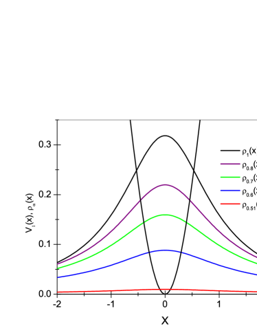
Figure 1: $\ln(1+x^{2})$ against $\rho_{\alpha}(x)$ with $1/2<\alpha\leq 1$.

To deduce the values of above dimensionless inverse temperature $\alpha$, we need an explicit expression for the mean value

$${\cal{U}}_{\alpha}=\langle{\cal{V}}\rangle_{\alpha}=\frac{\Gamma(\alpha)}{\sqrt{\pi}\Gamma(\alpha-1/2)}\int_{-\infty}^{\infty}\frac{\ln(1+x^{2})}{(1+x^{2})^{\alpha}}dx.$$ (7)

It turns out that it can be given in terms of digamma function $\psi(x)=d(\ln\Gamma)/dx$ abr . We get

$${\cal{U}}_{\alpha}=-\frac{2\pi}{\sin(2\pi\alpha)}+\psi(1-\alpha)-\psi\left(\frac{3}{2}-\alpha\right),\ \alpha>\frac{1}{2}.$$ (8)

The dependence of ${\cal{U}}_{\alpha}$ on $\alpha$ is reported in Fig. 2, where it is seen that this function is divergent at $\alpha=1/2$ (see also below) and decays monotonously at large $\alpha$. This decay is conrolled by an asymptotic expansion

$${\cal{U}}_{\alpha}\approx\frac{1}{2\alpha}+\frac{3}{8\alpha^{2}}+\frac{1}{4\alpha^{3}}+...,$$ (9)

which is also shown on Fig. 2. It is seen that decay of ${\cal{U}}_{\alpha}$ at large $\alpha$ obeys the inverse power law. It follows from Fig. 2 that the expansion (9) gives a very good approximation of ${\cal{U}}_{\alpha}$ for $\alpha>3$.

Figure 2: ${\cal{U}}_{\alpha}$ (curve 1) and its asymptotic expansion at large $\alpha$ (curve 2).

We note that, apparently, Eq. (8) involves another divergence problems, if we choose integer $\alpha$. This obstacle can be circumvented by transforming Eq. (8) to an equivalent form that has no (effectively removable) divergencies. Namely, we get

$${\cal{U}}_{\alpha}=-\pi\tan\pi\alpha+\psi(\alpha)-\psi\left(\frac{3}{2}-\alpha\right)$$ (10)

and the tangent contribution vanishes for integer $\alpha$. On the other hand, this expression shows that the divergence of ${\cal{U}}_{\alpha}$ at $\alpha\to 1/2$ originates from the first term in (10), as $\psi$ functions have finite values at this point. Near $\alpha=1/2$ the first term of Eq. (10) diverges as $(\alpha-1/2)^{-1}$, which is clearly seen in Fig. 2.

The preceding discussion shows that weak confinement properties of logarithmic potential manifest themselves in the fact that the corresponding (Cauchy family) equilibrium pdfs exist only for the semi-infinite range of (dimensionless) inverse temperatures $\alpha\in(1/2,+\infty)$. Note that for strongly confining potentials (like e.g. $V(x)\sim x^{2}$ or $x^{4}$) this is not the case as it follows from Eq. (2) that the normalizing integral $C^{-1}=\int_{-\infty}^{\infty}\exp[-\lambda V(x)]dx$ is convergent at any $\lambda$, so that the whole temperature range $[0,\infty)$ is allowed.

Let us turn to a quantitative discussion of an impact of weak confinement properties of the above logarithmic potentials on thermodynamical properties of a random system. To this end, we should focus our attention on the thermodynamic meaning of the (originally Lagrange multiplier) parameter $\alpha$ and its semi-bounded range of variability $(1/2,+\infty)$. This is also related to above problem of explicit calculation of $\alpha$ for a specific pdf.

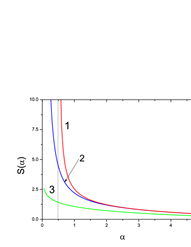
Figure 3: ${\cal{S}}_{\alpha}$ for Cauchy family (curve 1) and its asymptotic expansion at large $\alpha$ (curve 2) . ${\cal{S}}^{G}_{\alpha}$ for Gaussian family is also shown (curve 3).

With an explicit expression for Cauchy family pdfs (5) in hands, we readily evaluate Shannon entropy to obtain

$${\cal{S}}_{\alpha}=-\int_{-\infty}^{\infty}\rho_{\alpha}(x)\ln\rho_{\alpha}(x)dx=\ln Z_{\alpha}+\alpha\,{\cal{U}}_{\alpha}.$$ (11)

Then, the (as yet dimensionless) Helmholtz free energy ${\cal F}_{\alpha}$ reads

$${\cal{F}}_{\alpha}=\alpha{\cal{U}}_{\alpha}-{\cal{S}}_{\alpha}\equiv-\ln Z_{\alpha},$$ (12)

with $\alpha$ being the dimensionless inverse temperature, c.f. Ref. stat .

We note, that in view of the divergence of $Z_{\alpha}$, both the Shannon entropy and the Helmholtz free energy (likewise ${\cal{U}}_{\alpha}$) cease to exist at $\alpha=1/2$. We plot ${\cal{S}}_{\alpha}$ as a function of $\alpha$ in Fig.3. It is seen that entropy monotonously decays for $\alpha>1/2$ and for larger values of $\alpha$. An asymptotic expansion of the entropy shows logarithmic plus inverse power signatures

$${\cal{S}}_{\alpha}\approx\frac{1}{2}\left(1-\ln\frac{\alpha}{\pi}\right)+\frac{3}{4\alpha}+\frac{3}{8\alpha^{2}}+...$$ (13)

These series are shown along with the entropy in Fig. 3.

As $\alpha$ grows, the number of moments of respective pdfs increases. That allows to expect that an ”almost Gaussian” behavior should be displayed by $\alpha\gg 1$ members of Cauchy family (5). This is indeed the case. To this end, let us recall that the normalized Gaussian function with zero mean and variance $\sigma^{2}=1/2\alpha$ reads

$$\rho_{\alpha}^{G}(x)=\sqrt{\frac{\alpha}{\pi}}\ e^{-\alpha x^{2}}\equiv{\frac{1}{Z_{\alpha}^{G}}}e^{-\alpha x^{2}}.$$ (14)

The corresponding Shannon entropy gives exactly the first term of Eq. (13)

$${\cal{S}}^{G}_{\alpha}=\frac{1}{2}\ln\frac{\pi e}{\alpha}.$$ (15)

The plot of ${\cal{S}}^{G}_{\alpha}$ is reported in Fig.3 together with ${\cal{S}}_{\alpha}$ for Cauchy family. This equality suggests that at large $\alpha$ Cauchy family pdfs (5) transit to Gaussian one (14). This transition can be revealed if we rewrite Cauchy family pdfs (5) in the exponential form $\rho_{\alpha}(x)=\exp(\ln\rho_{\alpha})$ where $\ln\rho_{\alpha}=-\ln Z_{\alpha}-\alpha\ln(1+x^{2})$. It can be shown that at large $\alpha$ the ”tails” of pdf do not make substantial contribution so that only small $x$ play a role. This means that in limiting case of large $\alpha$ we can expand $\ln(1+x^{2})$ at small $x$. Then, employing series expansions

$$Z_{\alpha\to\infty}^{-1}\approx\sqrt{\frac{\alpha}{\pi}}-\frac{3}{8\sqrt{\pi\alpha}}-\frac{7}{128\alpha\sqrt{\pi\alpha}}-...$$ (16)

we arrive at

$$\rho_{\alpha}(x)\approx\left[\sqrt{\frac{\alpha}{\pi}}-\frac{3}{8\sqrt{\pi\alpha}}...\right]\,\exp\left(-\alpha x^{2}+\alpha\frac{x^{4}}{2}...\right)$$ (17)

whose leading order gives exactly the normalized Gaussian (14). Accordingly, c.f. Fig. 3, an inequality $\alpha>5$ sets a regime where a fairly good approximation of the Cauchy family pdfs by Gaussian is valid. Note that ultimately, in the $\alpha\to\infty$ limit, both families of functions (sequentially) approach the Dirac delta function(al).

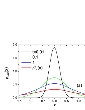
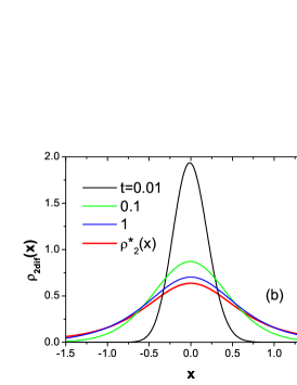
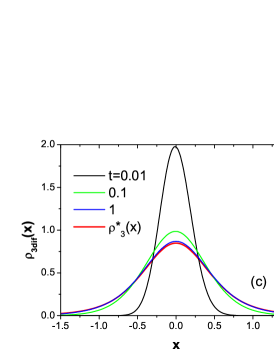
Figure 4: Time evolution of pdf’s $\rho(x,t)$ for Smoluchowski processes in logarithmic potential $\ln(1+x^{2})$. The initial ($t=0$) pdf is set to be a Gaussian with height 25 and half-width $\sim 10^{-3}$. The first depicted stage of evolution corresponds to $t=0.01$. Target pdfs are the members of Cauchy family (5) for $\alpha=1$ (panel (a)), 2 (panel (b)) and 3 (panel (c)) respectively.

Let us now show that the variational principle (1) explicitly identifies an equilibrium solution of the Fokker-Planck equation for standard Smoluchowski diffusion processes. To address our thermalization issue correctly, we now use dimensional units. The Fokker - Planck equation that drives an initial probability density $\rho(x,t=0)$ to its final (equilibrium) form $\rho(x,t\to\infty)$ reads

$$\partial_{t}\rho=D\Delta\rho-\nabla\cdot(b(x)\rho).$$ (18)

We still refer (although without substantial limitation of generality) to the 1D case, so that $\nabla\equiv\partial/\partial x$. Here, the drift field $b(x)$ is time-independent and conservative, $b(x)=-\nabla V(x)/(m\gamma)$ ($V(x)$ is a potential, while $m$ is a mass and $\gamma$ is a reciprocal relaxation time of a system). We keep in mind that $\rho$ and $b\rho$ vanish at spatial infinities or other integration interval borders.

If Einstein fluctuation-dissipation relation $D=k_{B}T/m\gamma$ holds, the equation (18) can be identically rewritten in the form $\partial_{t}\rho=\nabla[\rho\nabla\Psi]/(m\gamma)$, where

$$\Psi=V+k_{B}T\ln\rho$$ (19)

whose mean value is indeed the Helmholtz free energy of random motion

$$F\equiv\left<\Psi\right>=U-TS.$$ (20)

Here the (Gibbs) entropy reads $S=k_{B}{\cal{S}}$, while an internal energy is $U=\left<V\right>$. In view of assumed boundary restrictions at spatial infinities, we have $\dot{F}=-(m\gamma)\left<{v}^{2}\right>\leq 0$. Hence, $F$ decreases as a function of time towards its minimum $F_{*}$, or remains constant.

Let us consider the stationary (large time asymptotic) regime associated with an invariant density $\rho_{*}$ (c.f. mackey for an extended discussion of that issue). Then, $\partial_{t}\rho=0$ and we have $\nabla\Psi[\rho_{*}]=C\rho_{*}$ ($C$ is arbitrary constant) which yields

$$\rho_{*}={\frac{1}{Z}}\exp[-V/k_{B}T]\,.$$ (21)

Therefore, at equilibrium:

$$\Psi_{*}=V+k_{B}T\ln\rho_{*}\Longrightarrow\langle\Psi_{*}\rangle=-k_{B}T\ln Z\equiv F_{*},$$ (22)

to be compared with Eq. (12). Here, the partition function equals $Z=\int\exp(-V/k_{B}T)dx$, provided that the integral is convergent. Since $Z=\exp(-F_{*}/k_{B}T)$ we have recast $\rho_{*}(x)$ in the familiar Gibbs-Boltzmann form $\rho_{*}=\exp[(F_{*}-V)/k_{B}T]$.

On physical grounds, $V(x)$ carries dimensions of energy. Therefore to establish a physically justifiable thermodynamic picture of Smoluchowski diffusion processes, relaxing to Cauchy family pdfs in their large time asymptotics, we need to assume that logarithmic potentials ${\cal{V}}(x)=\ln(1+x^{2})$ are dimensionally scaled to the form $V(x)=\epsilon_{0}{\cal{V}}$ where $\epsilon_{0}$ is an arbitrary constant with physical dimensions of energy.

By employing $(1/\epsilon_{0})\,V(x)=\ln(1+x^{2})$, we can recast previous variational arguments (MEP procedure) in terms of dimensional thermodynamical functions. Namely, in view of $k_{B}T\Phi(x)=V(x)+k_{B}T\,\ln\rho(x)$ we have an obvious transformation of Eqs. (3), (5) and (12) into Eqs. (20),(21) and (22) respectively with $k_{B}T\Phi(x)=\Psi(x)$.

The above dimensional arguments tell us that in weakly confining logarithmic potentials, Cauchy family of pdfs can be regarded as a one-parameter family of equilibrium pdfs, where the reservoir temperature $T$ enters through the exponent $\alpha$. Proceeding in this vein, we note that $\epsilon_{0}$ should be regarded as a characteristic energy (energy scale) of the considered random system.

We observe that $\alpha\to\infty$ corresponds to $T\to 0$ i.e. a maximal localization (Dirac delta limit) of the corresponding pdf. In parallel ${\cal{S}}(\alpha\to\infty\equiv T\to 0)\to 0$ and an analogy with the Nernst theorem is established.

The opposite limiting case $\alpha\to 1/2$ looks interesting as well. Namely, we have ${\cal{S}}(\alpha\to 1/2)\to\infty$. To grasp the meaning of this limiting regime, we rewrite $\alpha=1/2$ in the form $k_{B}T=2\epsilon_{0}$. Accordingly, the temperature scale, within which our system may at all be set at thermal equilibrium, is bounded: $0<k_{B}T<2\epsilon_{0}$. For temperatures exceeding the upper bound $T_{max}=2\epsilon_{0}/k_{B}$ no thermal equilibrium is possible in the presence of (weakly, i.e. weaker then, e.g., $V(x)\sim x^{2}$ ) confining logarithmic potentials $V(x)=\epsilon_{0}\,\ln(1+x^{2})$. The case of $\alpha=1$ i.e. $k_{B}T=\epsilon_{0}$ corresponds to Cauchy density.

Let us finally add that in Ref. gar , we have analyzed diffusion processes in logarithmic potentials, with a focus on temporal relaxation patterns of the process towards asymptotic pdfs from the Cauchy family. For clarity of presentation (dynamical interpolation scenarios between initial Gaussian and equilibrium Cauchy-type pdfs do not seem to have ever been considered in the literature), in Fig. 4 we plot various stages of the diffusive Fokker - Planck dynamics for processes that all have been started from a narrow Gaussian. It turns out that the the resultant (large time asymptotic) equilibrium pdfs are members of Cauchy family (5), labeled respectively by $\alpha=1$, $2$ and $3$.

References

- (1) M. C. Mackey, Time’s arrow: The origins of thermodynamic behavior, Springer-Verlag, Berlin, 1992
- (2) J. N. Kapur and H. K. Kesavan, Entropy Optimization Principles with Applications, Academic Press, Boston, 1992
- (3) P. Garbaczewski, V. Stephanovich and D. Kȩdzierski, Non-Gaussian targets and (ab)normal patterns of relaxation in random motion, arXiv:1004.0127, (2010)
- (4) P. Garbaczewski and V. Stephanovich, Phys. Rev. E 80, 031113, (2009)
- (5) P. Garbaczewski, Entropy, 7 [4], 253-299, (2005)
- (6) M. Abramowitz and I. A. Stegun, Handbook of mathematical functions, Dover, NY, 1970
- (7) M. C. Mackey and M. Tyran-Kamińska, Physica A, 365, 360-382, (2006)