Persistent Evidence of a Jovian Mass Solar Companion in the Oort Cloud

PROPOSED RUNNING HEAD
“Jovian Mass Solar Companion in the Oort Cloud”

EDITORIAL CORRESPONDENCE AND PROOFS
John J. Matese
Department of Physics
University of Louisiana at Lafayette
Lafayette, LA, 70504-4210
Tel: (337) 482 6697
Fax: (337) 482 6699
E-mail: matese@louisiana.edu

Abstract: We present an updated dynamical and statistical analysis of outer Oort cloud cometary evidence suggesting the sun has a wide-binary Jovian mass companion. The results support a conjecture that there exists a companion of mass $\approx 1-4\;{\rm M_{Jupiter}}$ orbiting in the innermost region of the outer Oort cloud. Our most restrictive prediction is that the orientation angles of the orbit normal in galactic coordinates are centered on $\Omega$, the galactic longitude of the ascending node = 319^∘ and $i$, the galactic inclination = 103^∘ (or the opposite direction) with an uncertainty in the normal direction subtending $\approx 2\%$ of the sky. A Bayesian statistical analysis suggests that the probability of the companion hypothesis is comparable to or greater than the probability of the null hypothesis of a statistical fluke. Such a companion could also have produced the detached Kuiper Belt object Sedna. The putative companion could be easily detected by the recently launched Wide-field Infrared Survey Explorer (WISE).

Key Words: Comets, dynamics; Celestial mechanics; Kuiper Belt; Jovian planets; Planetary dynamics

1 Introduction

Anomalies in the aphelia distribution and orbital elements of Outer Oort cloud comets led to the suggestion that $\approx$ 20% of these comets were made discernable due to a weak impulse from a bound Jovian mass body (Matese et al. (1999)). Since that time the data base of comets has doubled. Further motivation for an updated analysis comes from the recent launch of the Wide-field Infrared Survey Explorer (WISE; (2007)), which could easily detect the putative companion orbiting in the outer Oort cloud. Such an object would be incapable of creating comet “storms”. To help mitigate popular confusion with the Nemesis model (Whitmire and Jackson (1984), Davis et al. (1984)) we use the name recently suggested by Kirkpatrick and Wright (2010), Tyche, (the good sister of Nemesis) for the putative companion.

The outer Oort cloud (OOC) is formally defined as the ensemble of comets having original semimajor axes $A\geq 10^{4}$ AU (Oort (1950)). It has been shown that the majority of these comets that are made discernable are first-time entrants into the inner planetary region (Fernandez (1981)) and these comets are therefore commonly referred to as new. The dominance of the galactic tide in making OOC comets discernable at the present epoch has been predicted on theoretical grounds (Heisler and Tremaine (1986)). Observational evidence of this dominance has been claimed to be compelling (Delsemme (1987); Matese and Whitman (1992); Wiegert and Tremaine (1999); Matese and Lissauer (2004)).

Matese and Lissauer (2004) adopted an in situ energy distribution similar to the initial distribution of Rickman et al. (2008) and took the remaining phase space external to a “loss cylinder” to be uniformly populated at the present epoch. The distribution of cometary orbital elements made discernable from the tide alone was then obtained and compared with observations.

Similar modeling (Matese and Lissauer (2002)) had been performed including single stellar impulses which mapped the comet flux over a time interval of 5 Myr, in 0.1 Myr intervals. Peak impulsive enhancements $\geq 20\%$ were found to have a half-maximum duration of $\approx 2$ Myr and occurred with a mean time interval of $\approx 15$ Myr. Various time-varying distributions of elements were compared with the modeled tide-alone results and inferences about the signatures of a weak stellar impulse were drawn.

In Section 2 we review a discussion (Matese and Lissauer (2004)) of a subtle characteristic of galactic tidal dominance which is difficult to mimic with observational selection effects or bad data. Along with the more well known feature of the deficiency of major axis orientations in the direction of the galactic poles and equator, we compare with observations these predictions based on the tidal interaction alone and show that the data are of sufficiently high quality to unambiguously demonstrate the dominance of the galactic tide in making comets discernable at the present epoch. A critique of objections to this assertion (Rickman et al. (2008)) is also presented. More recent detailed modeling (Kaib and Quinn (2009)) provide important insights into the evolving populations of the in situ and discernable populations of the Oort cloud. We comment further on these works in this section.

In Section 3 we describe the theoretical analysis combining a secular approximation for the galactic tide and for a point mass perturber, describing how a weak perturbation of OOC comets would manifest itself observationally. Evidence suggesting that there is such an aligned impulsive component of the observed OOC comet flux has been previously reported (Matese et al. (1999)). It has been found that none of the known observational biases can explain the alignment found there (Horner and Evans (2002)). The size of the available data has since doubled which leads us to review the arguments here.

In Section 4 we present the supportive evidence that an impulsive enhancement in the new comet flux of $\approx 20\%$ persists in the updated data. We also discuss dynamical and observational limits on parameters describing the putative companion. Section 5 summarizes our results and presents our conclusions.

2 Secular dynamics of the galactic tide

Near-parabolic comets are most likely to have their perihelia reduced to the discernable region. The dynamics of the galactic tide acting on near-parabolic OOC comets is most simply described in a Newtonian framework (Matese et al. (1999), Matese and Lissauer (2002), Matese and Lissauer (2004)). A summary of their analyses is now given and followed with the evidence that the galactic tidal perturbation dominates in making OOC comets discernable at the present epoch.

2.1 Theory

Saturn and Jupiter provide an effective dynamical barrier to the migration of OOC comet perihelia. OOC comets that are approaching the planetary zone at the present time were unlikely to have had a prior perihelion, $q_{prior}$, that was interior to the “loss cylinder” radius, $q_{lc}\approx 15$ AU, when it left the planetary region on the present orbit. The simplifying assumption $q_{lc}\leq q_{prior}$ is then made for the present orbit. During the present orbit comet perihelion will then have been changed by the galactic tide (and by any putative companion or stellar perturbation). The orbital elements just before re-entering the planetary region on the present orbit are commonly referred to as “original” and will be, in essence, the observed values with the exception of the semimajor axis (perturbations by the major planets do not significantly change any other orbital element of OOC comets). Thus $q_{prior}$ is changed to $q_{original}\approx q_{obs}$, the observed value, during the course of the present orbit. As an observed comet comes within a discernable region ($q_{obs}\leq q_{discernable}\approx 5$AU) and leaves the planetary region again, the semimajor axis will have been changed from $A_{original}$ to $A_{future}$, i.e., $A_{future}\equiv A_{prior}$ for the next orbit. The comet is most likely ejected or turned into an inner Oort cloud comet with a small fraction returning as OOC comets. Daughter comets returning to the discernable zone are likely to have faded and be more difficult to observe (Wiegert and Tremaine (1999)). The $17th$ Catalogue of Cometary Orbits (Marsden and Williams (2008)) indicates that $\approx 14\%$ of observed original OOC comets exit the planetary region as future OOC comets. Therefore the discernable population of OOC comets should be dominated by first time entrants to the loss cylinder. In the following we adopt the notation $A\equiv A_{original}$.

For near-parabolic comets, the angular momentum per unit mass determines the perihelion distance, $\mathbf{H}\equiv\mathbf{R}\times{\dot{\mathbf{R}}}$, ($\mathbf{H}\perp\mathbf{q},\;H\approx\sqrt{2\mu_{\odot}q}$). With these assumptions, an observed OOC comet entering the loss cylinder region for the first time had perihelion distances $q_{obs}\leq q_{discernable}<q_{lc}\leq q_{prior}$. Therefore, reducing $q$ in a single orbit requires a decrease in angular momentum from the galactic tidal torque (and/or from angular momentum changes by the putative companion or star),

$$\Delta\mathbf{H}\equiv\mathbf{H_{obs}}-\mathbf{H_{prior}}\;\textrm{, or,}\;\;\;q_{prior}-q_{obs}=\left(\mathbf{\Delta H}^{2}-2\mathbf{H_{obs}}\cdot\mathbf{\Delta H}\right)/2{\mu_{\odot}}.$$ (1)

The weakest perturbation that could make a comet discernable would reduce the prior perihelion distance from $q_{prior}\approx q_{lc}$ to $q_{obs}\approx q_{discernable}$ (see Fig. 1) such that

$${|\Delta\mathbf{H}|}_{min}=\sqrt{2\mu_{\odot}\;q_{lc}}-\sqrt{2\mu_{\odot}\;q_{discernable}}\;\;.$$ (2)

Also of interest is the evolution of the aphelion orientation, ${\mathbf{\hat{Q}}}\equiv~{}({\cos B}\;{\cos L},{\cos B}\;{\sin L},\sin B)$, expressed in terms of the aphelion latitude, $B$, and longitude, $L$.

If the galactic tide dominates in making OOC comets discernable we can recast Eq. (1) as $q_{prior}-q_{obs}=\left(\mathbf{\Delta H_{tide}}^{2}-2\mathbf{H_{obs}}\cdot\mathbf{\Delta H_{tide}}\right)/2{\mu_{\odot}}$ from which it is implied that if weak tidal perturbations dominate in making OOC comets discernable, the tidal characteristic, $S\equiv{\rm Sign}(\mathbf{H_{obs}}\cdot\Delta\mathbf{H_{tide}})$ will more often be $\;-1$ than +1. Detailed modeling results (Matese and Lissauer (2004)) confirm this implication. This characteristic combination of observed orbital elements forms an essential aspect of the present analysis and has not been included in modeling results presented elsewhere (e.g., Rickman et al. (2008), Kaib and Quinn (2009)).

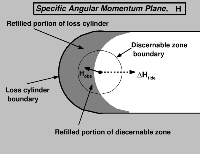
Fig. 1: Schematic illustration of the plane of specific angular momentum phase space, $\mathbf{H}$, for a given $A$ and $\mathbf{\widehat{Q}}$, the aphelion direction defining the normal to this plane. Phase space points illustrated have the same values of $A$, $B$, and $L$, but cover the entire region of $\mathbf{H}$ just outside the loss cylinder. Light gray shaded region outside the loss cylinder boundary ($H>H_{lc}\propto\sqrt{q_{lc}}$) denotes the filled phase space of comets leaving the planetary region on their prior orbits. The uniform displacement of all phase space points one orbit later by a tidal perturbation $\mathbf{\Delta H_{tide}}$ is shown partially refilling the loss cylinder region (indicated as the dark gray region). The discernable zone within the loss cylinder ($H<H_{discernable}\propto\sqrt{q_{discernable}}$) is indicated. It remains unfilled for negligible perturbations of small-$A$ comets, becomes totally refilled for strong perturbations of large-$A$ OOC comets, and, as illustrated here, is partially refilled for weak perturbations of intermediate-$A$ OOC comets. The tidal characteristic $S\equiv{\rm Sign}(\mathbf{H_{obs}}\cdot\Delta\mathbf{H_{tide}})=-1$ for all observed comets in the refilled portion of the discernable phase space here. Over successive orbits the loss cylinder and its shadow region of unfilled phase space (shaded white) will be depleted for small-$A$ and intermediate-$A$ OOC comets.

A graphical illustration of this theme in Fig. 1 shows the phase space changes in $\mathbf{H}$ for a specific choice of $\mathbf{\widehat{Q}}$ and $A$ over the course of a single orbit period. As comets recede from the planetary region on their prior orbits, the interior of the loss cylinder phase space region is essentially emptied of OOC comets by planetary perturbations. The adjacent exterior region remains uniformly populated in this model. To lowest order in $q/A$, i.e., the near-parabolic phase space region just outside the loss cylinder boundary, the vector displacement in specific angular momentum, $\mathbf{\Delta H_{tide}}$, is independent of the prior value of angular momentum, $\mathbf{H_{prior}}$, and depends only on $A$ and the major axis orientation, $\mathbf{\widehat{Q}}$, which are taken to be fixed for the phase space of Fig. 1. In a single orbit all nearby specific angular momentum phase space points, filled and empty, are displaced uniformly (Matese and Lissauer (2004)). Figure 1 illustrates that in the present modeling, the phrase “loss cylinder” might be more appropriately changed to “loss circle”. It also indicates that the phrase “loss cone” which is commonly used in describing impulsive domination is no longer appropriate if the tide dominates.

The magnitude of the single-orbit angular momentum displacement is strongly dependent on $A$, varying as $A^{7/2}$. Small-$A$ comets are defined here as having negligible galactic perturbations, $<{|\Delta\mathbf{H}|}_{min}$, unable to repopulate the discernable zone with new comets. This includes the inner Oort cloud (IOC), but also overlaps with the smallest-$A$ population of the formal OOC. Large-$A$ OOC comets are defined here as those having strong tidal perturbations resulting in large displacements in $\mathbf{H}$ that completely refill the discernable zone, making $S=\mp 1$ equally likely. Intermediate-$A$ OOC comets are defined here as those that are weakly perturbed by the tide and only partially refill the discernable zone. Intermediate-$A$ comets preferentially have $S=-1$, as seen in Fig. 1. In this context intermediate-$A$ OOC comets have the smallest observed values of $A$ among the OOC comets if the tide alone makes the comets discernable. The fuzzy boundaries between small-$A$, intermediate-$A$ and large-$A$ depend weakly on $B$ and $L$. We choose the boundaries for these intervals based on data discussed in Section 3.

Therefore, independent of stellar influences on the in situ distribution of semimajor axes, if the galactic tidal interaction with the OOC dominates impulsive interactions in making OOC comets discernable at the present epoch we should see

• a preponderance of OOC comets with $S=-1$ over those with $S=+1$, and

• an association in which $S=-1$ correlates with the smallest observed values of $A$ for OOC comets.

Conversely, if perturber impulses dominate in making OOC comets discernable at the present epoch, the unique tidal characteristic $S$ should be a random variable and should be uncorrelated with $A$.

2.2 Observational evidence for tidal dominance at the present epoch

Our data are taken from the $17th$ Catalogue of Cometary Orbits from which we convert the ecliptic Eulerian orbital angles into the galactic angles $B$, $L$ and $\alpha$, the orientation angle of $\mathbf{H}$ defined in Matese and Lissauer (2004). The Catalogue lists 102 OOC comets (see Appendix) of the highest quality class, 1A (we count the split comet C/1996-J1A(B) as a single comet). The quality class predominantly distinguishes the accuracy of the original semimajor axis determination (Marsden et al. (1978)). Since our analysis depends sensitively on an accurate determination of $A$, we restrict our detailed discussions to class 1A comets. In a previous analysis (Matese et al. (1999)) the orbital elements of 82 OOC comets of quality classes 1A+1B given in the 11th Catalogue were used, 47 of which were class 1A.

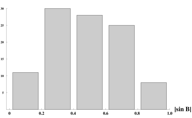
Fig. 2: The distribution in $|\sin B|$ for class 1A new comets.

The first observational indication that the galactic tide dominates involved the distribution in the galactic latitude of aphelion, $B$ (Delsemme (1987)). One finds (Matese et al. (1999)) that the dominant disk tidal term in the perturbation is $\propto|\sin B\cos B|$. (Rickman et al. (2008) conclude that this perturbation is $\propto|\sin B|$ rather than $\propto|\sin B\cos B|$). $B$ and $L$ are sensibly constant in the course of a single orbit since $\mathbf{Q}$ has significant inertia for near-parabolic orbits. Therefore, if the tide dominates we should expect deficiencies of major axis orientations along the galactic poles and the galactic equator, and peaks near $B=\pm 45^{\circ}$. One might argue that observational selection effects can artificially produce an equatorial gap, but polar gaps will be more difficult to attribute to an observational selection effect.

In Fig. 2 we show the results presented as a distribution in $|\sin B|$, which would be uniform for a random distribution. Polar and equatorial gaps are clear, as predicted if the galactic tide dominates. A small (but potentially informative) discrepancy is the location of the peak. If the tide dominates, our modeling (Matese and Lissauer (2004)) predicts a peak at $|\sin B|\approx 0.7$, somewhat larger than seen in the data. We now look to the tidal characteristic $S$ to further emphasize tidal dominance.

Fig. 3: The cumulative binding energy distribution ($x\equiv 10^{6}$ AU/$A$) separately illustrated for $S=\mp 1$. Solid line $\leftrightarrow$ $S=-1$, dotted line $\leftrightarrow$ $S=+1$.

The prediction that $S=\mp 1$ should be equally likely for large-$A$ OOC comets, and that there should be a preponderance of $S=-1$ for intermediate-$A$ OOC comets (see Fig. 1) is now considered. In terms of the original orbital binding energy parameter $x\equiv 10^{6}$ AU/$A$, class 1A OOC comets have a mean formal error of $\approx$ 5 units, but the uncertainty due to unmodeled outgassing effects is likely to be somewhat larger (Kresák (1992), Królikowska (2006)). In particular the number of nominally unbound original orbits is likely indicative of the true errors embodied in the tails of the class 1A OOC energy distribution.

In Fig. 3 we show the cumulative class 1A binding energy distribution of 66 comets with $S=-1$ and 36 comets with $S=+1$. The binomial probability that as many or more would exhibit this imbalance if in fact $S=\mp 1$ were equally likely is $2\times 10^{-3}$. Further, as predicted by tidal dynamics, this preponderance of $S=-1$ also correlates with intermediate-$A$ OOC comets in a statistically significant manner. $S=\mp 1$ is approximately equally likely for comets with $x\leq 30$, suggesting that for this range of semimajor axes the galactic tide is strong enough to refill the discernable zone almost completely, i. e., the tidal efficiency is nearly $100\%$ (Matese and Lissauer (2002)). We therefore take this as the defining boundary between large-$A$ and intermediate-$A$ comets. In contrast, for $30<x$ the evidence is that the tide weakens dramatically since 45 comets have $S=-1$ and only 12 have $S=+1$. The binomial probability that as many or more would exhibit this imbalance if in fact $S=\mp 1$ were equally likely for this energy range is $7\times 10^{-6}$. This is unambiguous evidence that the class 1A data are of sufficiently high quality and sufficiently free of observational selection effects to detect this unique imprint of tidal dominance in making OOC comets discernable at the present epoch.

Kaib and Quinn (2010) have found that $\approx 5\%$ of discernable OOC comets should have $60<x$, the majority of which have evolved from a primordial location in the IOC. It is unlikely that these comets have had their prior orbit perihelia outside the loss cylinder and therefore would not satisfy ${|\Delta\mathbf{H}|}>{|\Delta\mathbf{H}|}_{min}$. Taking account of expected errors in the binding energies we adopt $30<x<60$ as the defining interval for intermediate-$A$ comets.

These clear signatures of galactic tidal dominance in making OOC comets discernable do not mean that we must abandon hope for detecting any impulsive imprint on the distributions, as we describe in Sec 3. The characteristic $S=-1$ continues to dominate for observed IOC comets, suggesting that they are likely to be daughters of OOC comets. $S=-1$ also remains dominant for other quality class OOC data (1B, 2A, 2B). However the dominance no longer correlates with the energy range $30<x$. We interpret this as evidence of significant errors in the determination of $A$ for these quality classes, a conclusion made clear by the excess of nominally unbound comets.

2.3 Comparisons with recent modeling

Kaib and Quinn (2009) have done the most complete modeling of the production of observable long-period comets (LPC) from the Oort cloud in an attempt to infer the Sun’s birth environment. They closely follow whether an observed OOC comet was born in the OOC or in the IOC and find that roughly comparable numbers of each primordial population are made discernable after a suitable time lapse. Their binding energy distribution for the two discernable populations (their Fig. S4) differs in that the distribution for comets born in the IOC peaks at $x\approx 37$ while the peak for comets born in the OOC peaks at $x\approx 27$. They conclude that the IOC pathway provides “an important, if not dominant, source of known LPCs”. The primordial origin of discernable comets is not important in our loss-cylinder modeling. The $17th$ Catalogue indicates that only 2 of the 53 observed class 1A comets with $100<x<1000$ have future orbits in the OOC, while 14 of 102 observed class 1A OOC comets that have future orbits in the OOC. Therefore very few observed comets with $30<x<60$ are likely to have prior perihelia within the loss cylinder. We have used their Fig. S4 as a guide to the energy range most likely to show evidence of a weak impulsive component of the observed OOC.

Rickman et al. (2008) have also embarked on an ambitious modeling program of the long term evolution of the Oort cloud which emphasizes a fundamental role for stellar perturbations. They demonstrate that over long timescales stellar impulses are needed to replenish the phase space of the OOC which is capable of being made discernable by the galactic tide. Massive star impulses serve to efficiently refill this feeding zone for a period of several 100 Myr and therefore provide one aspect of the synergy with the galactic tide that make these comets discernable.

They also assert that “treating comet injections from the Oort cloud in the contemporary Solar System as a result of the Galactic tide alone is not a viable idea”. This statement follows from their observations that a tide-alone model evolving over the lifetime of the Solar System differs significantly at the present epoch from a combined impulse-tide model.

But their modeling does not shed light on the question of the dominant dynamical mechanism responsible for injecting OOC comets into the inner planetary region at the present epoch. Their work makes detailed predictions using results averaged over 170 Myr. Such a large time window inevitably includes many individual stellar perturbations which contribute directly to the time-averaged flux. Separating out the dominant perturbation making these comets discernable at the present epoch would be best obtained if they (i) “turn off” both perturbations at the present epoch, (ii) wait for the discerned flux to dissipate, and then (iii) alternately determine subsequent distributions produced by each perturbation separately turned on. This analysis was not performed.

Indeed, one can compare our predictions (Matese and Lissauer (2004)) for discernable distributions in $A$ and the $A$-dependent discernable zone refill efficiency with Rickman et al. (2008) (where they use the term “filling factor” in the same context as our “efficiency”). The tide-alone results at the beginning of their simulations (see their Fig. 7 and Table III) provide the most appropriate comparison since their phase space then is most nearly randomized and comparable to that used in our previous work. One finds that these two sets of distributions are in good agreement.

Their combined modeling of the latitude distributions does predict a peak at $|\sin B|\approx 0.5$, more nearly in agreement with observations shown in Fig. 2 (however they assert that their predictions do not agree with observations without any discussion of the nature of the discrepancies perceived). If this difference with our tidal model prediction of a peak at $|\sin B|\approx 0.7$ is supported in the future it may provide evidence that the in situ phase space refilling by stellar perturbations is indeed detectably incomplete at the present epoch, a point emphasized by them. This would not contradict our assertion that the unambiguous evidence is that the galactic tide dominates in making OOC comets discernable at the present epoch. It remains for them to demonstrate that the modeling adopted here (Matese and Lissauer (2002, 2004)) is no longer viable in describing observations at the present epoch. We conclude our remarks by noting that neither of the above analyses have tracked the orbital characteristic $S$ in the production of discernable OOC, a major measure of galactic dominance in our work.

3 Dynamics of a weak impulsive perturbation

3.1 Theory

The dynamics of a weak perturbation of a near-parabolic comet by a solar companion or field object is now considered. The change in the comet’s specific heliocentric angular momentum induced by a perturber is given by

$$\mathbf{\dot{H}_{pert}}=\mu_{p}\left(\mathbf{R}\times\mathbf{r}\right)\left(\frac{1}{|\mathbf{R}-\mathbf{r}|^{3}}-\frac{1}{r^{3}}\right)$$ (3)

where $\mu_{p}={\rm G}M_{p}$ is the perturber mass located at heliocentric position $\mathbf{r}$ and $\mathbf{R}$ is the heliocentric comet position. In terms of the perturber true anomaly, $f$, we have $r=p/(1+e_{p}\cos f),$ with $p=a(1-{e_{p}}^{2})$. We then obtain for near-parabolic comets

$$\frac{d\mathbf{H_{pert}}}{df\;\;\;\;\;}=\sqrt{\mu_{\odot}a}\;\frac{\mu_{p}}{\mu_{\odot}}\;\left(\mathbf{\widehat{Q}}\times\mathbf{\hat{r}}\right)\;\frac{R}{b}\;\left(\frac{r^{3}}{|\mathbf{R}-\mathbf{r}|^{3}}-1\right)$$ (4)

where $b=a\sqrt{1-{e_{p}}^{2}}$, the semiminor axis of the perturber. One then constructs

$$\Delta\mathbf{H_{pert}}=\sqrt{\mu_{\odot}a}\;\frac{\mu_{p}}{\mu_{\odot}}\;\mathbf{\widehat{Q}}\times\mathbf{I},$$ (5)

where the dimensionless integral $\mathbf{I}$ is taken around an interval of the perturber true anomaly $\Delta f\equiv f_{o}-f_{i}$ that corresponds to the comet orbital time interval between $t_{o}\equiv 0$, the present epoch, and $t_{i}\equiv-2\pi\sqrt{A^{3}/\mu_{\odot}}$,

$$\mathbf{I}\equiv{\int_{f_{i}}}^{f_{o}}\;df\;\mathbf{\hat{r}}\;\frac{R}{b}\;\left(\frac{r^{3}}{|\mathbf{R}-\mathbf{r}|^{3}}-1\right).$$ (6)

The first term in $\mathbf{I}$ corresponds to the perturber interaction with the comet, the second with the Sun. For a specified perturber orbital ellipse, $\mathbf{I}$ is determined by the cometary $\mathbf{\widehat{Q}}$ and $A$ as well as the companion’s present value of the true anomaly, $f_{o}$. Equation  3 is more convenient to use in an impulse approximation as has been done in a previous analysis of the combined tide-stellar impulse interaction with the OOC (Matese and Lissauer (2002)). Equation  4 is more appropriate if one wishes to include the slow “reflex” effects of a bound perturber on the Sun.

3.2 Combined tidal and impulsive interaction

The galactic tidal perturbation and any putative point source perturbation of the Sun/OOC are, in nature, superposed in the course of a cometary orbit. For weak perturbations the two effects can be superposed in a vector sense, $\mathbf{H_{obs}}\equiv\mathbf{H_{prior}}+\mathbf{\Delta H_{pert}}+\mathbf{\Delta H_{tide}}\equiv\mathbf{H_{prior}}+\mathbf{\Delta H_{net}}.$ The cometary phase space of comets will have the prior loss cylinder distribution displaced by $\mathbf{\Delta H_{net}}$. The standard step function for the prior distribution of angular momentum is changed to a uniformly displaced distribution, similar to that illustrated in Fig. 1, but with $\mathbf{\Delta H_{tide}}$ replaced by $\mathbf{\Delta H_{net}}$, $q_{prior}-q_{obs}=\left(\mathbf{\Delta H_{net}}^{2}-2\mathbf{H_{obs}}\cdot\mathbf{\Delta H_{net}}\right)/2{\mu_{\odot}}.$

3.3 Weak impulsive effects on the discernable energy and spatial distributions

Matese and Lissauer (2002) modeled the time-dependent changes in discernable OOC comet orbital element distributions that resulted from a weak stellar impulse. In particular, the in situ energy distribution was taken to be essentially unchanged, as described above. The number of comets in the large-$A$ ($x\leq 30$) interval that became discernable after an impulse was found to be essentially unchanged from the case with no impulse, although the specific comets made discernable were changed. That is, the $\approx 100\%$ efficiency of refilling the discernable zone remains $\approx 100\%$ throughout the stellar impulse for large-$A$ comets. This can be visualized in Fig. 1 when we consider a large $\mathbf{\Delta H_{tide}}$ that completely refills the loss cylinder and the comparative case where the large $\mathbf{\Delta H_{tide}}$ is modified by a weak $\mathbf{\Delta H_{pert}}$. Independent of whether the impulse slightly increased or decreased the perturbation, a large $|\mathbf{\Delta H_{net}}|$ will still tend to completely refill the loss cylinder, albeit with different comets.

For the intermediate-$A$ population the discussion is more subtle. Suppose that for a specific $\mathbf{\widehat{Q}}$ a comet population with $x\approx 35$ will partially fill the discernable zone due to the tide (see Fig. 1). If some of those comets experience an impulse that increases $|\mathbf{\Delta H_{net}}|$, the discernable zone will be more completely filled. However other comets will be impulsed such that $|\mathbf{\Delta H_{net}}|$ is decreased. This will in turn decrease the number of discernable comets for this value of $x$ leaving the efficiency for this $x$ only moderately increased.

Consider now the case for a population with $x\approx 45$. The tidal perturbation will be smaller by a factor of $\approx 0.4$ from the $x\approx 35$ population, which may be inadequate to make any of these comets discernable in our loss cylinder model. In this case an impulsive torque preferentially opposed to the tidal torque will have no effect on the number of observed comets for this $x$ since none would have been observed in its absence. But for those comets which have a weak impulsive torque preferentially aiding the tide, some will be made discernable that would not have been in the absence of an impulse. Therefore the efficiency for this $x$ will increase from zero, and it will preferentially have $S=-1$. The net effect for a weak impulse is to create an enhanced observed OOC comet population along the track of the perturber that preferentially has intermediate-$A$ and $S=-1$. These features have been demonstrated in detailed modeling for a weak stellar impulse (Matese and Lissauer (2002)). Rickman et al. (2008) also discuss in detail this aspect of synergy but do not consider the importance of the characteristic, $S$, in this discussion.

In reality, the step function distribution of prior orbits for OOC comets used in the loss cylinder model is a crude first approximation. A small fraction of original OOC comet orbits recede from the planetary region as future OOC comets with perihelia inside the loss cylinder. This does not obviate the arguments invoked above. Along with the original energy errors associated with observational uncertainties and outgassing effects, we can understand why the observed spread in original energies seen in Fig. 3 is somewhat larger than predicted in our loss cylinder model and is consistent with more realistic modeling (Kaib and Quinn (2009)).

4 Observational evidence for an impulse

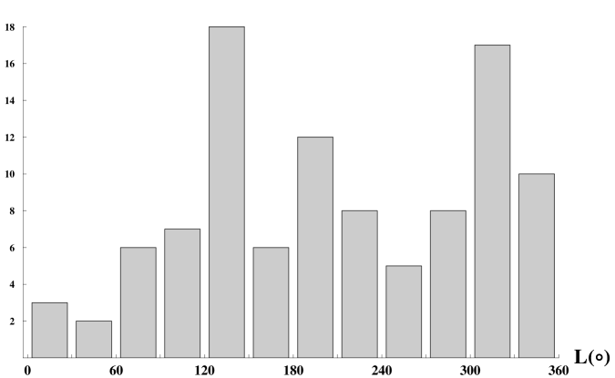
Fig. 4: The distribution of aphelia longitude, $L$, for class 1A OOC comets.

Matese et al. (1999) noted an excess of OOC comet major axes along a great circle roughly centered on the galactic longitudinal bins $135^{\circ}$ and $315^{\circ}$ using 11th Catalogue data of quality classes 1A+1B. Further, they found that the excess was predominantly in the intermediate-$A$ population and had a larger proportion of $S=-1$, consistent with it being impulsively produced. In Fig. 4 we now display the distribution of the aphelia longitudes for our $17th$ Catalogue data of quality class 1A. We see that the excess remains in the present data.

4.1 Inferring the orbit orientation of a putative bound perturber

Our first investigation relates to the orientation of the overpopulated band. There is no obvious a priori reason why an impulsive track should pass through the galactic poles. Further, choosing longitude bins for comparison has an obvious bias in that it preferentially excludes solid angles near the poles where the tide is weak.

We therefore perform a great circle fit that counts the number of major axes within an annular band of width $\pm 9.6^{\circ}$, which has the same solid angle, $4\pi/6$, as the two overpopulated aphelia longitude bins in Fig. 4. The data that we now analyze includes the 35 (of 102) $17th$ Catalogue comets listed in the Appendix which are intermediate-$A$ comets, $30<x<60$, with $S=-1$. As described above, this is the subset most likely to exhibit evidence of a weak impulsive component. Of these 35 comets, 15 were included in the $11th$ Catalogue considered by Matese et al (1999). Counting is done for all possible great circle orientations with normal directions stepped in a grid covering solid angles $\left({\frac{1}{2}}^{\circ}\right)^{2}$. The process is repeated for the $11th$ Catalogue data, the complete $17th$ Catalogue data as well as for the 20 comets in the $17th-11th$ Cataogue subset. Great circle orientations are denoted by the galactic longitude of ascending node, $\Omega$, and the galactic inclination, $i$. A similar plot holds for opposite great circle normal vectors $180^{\circ}-i$ with $\Omega-180^{\circ}$.

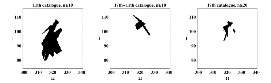
Fig. 5: Orientation angles ($\Omega$ =galactic longitude of ascending node, $i$= galactic inclination) of great circle bands of width $\pm 9.6^{\circ}$ which include 10(20) or more major axes of intermediate-$A$ comets with $S=-1$ .

For the $11th$ Catalogue data we can find a great circle with as many as 13 (of 15) axes inside the band. We show all orientations which include 10-13 major axes in Fig. 5. For the $17th-11th$ data we show all orientations that include 10-11 (of 20) major axes. One observes that the peak overpopulated great circle normal direction occurs in the same general area of the hemisphere for both the $11th$ and $17th-11th$ data. The probability that these solid angles would overlap if the two sets of data were uncorrelated can be estimated to be $\approx 0.02$. For the $17th$ Catalogue data we show those directions that include 20-22 (of 35) major axes. The statistical significance of these observations is discussed below.

The best fit great circle normal direction with a $\pm 9.6^{\circ}$ band containing 22 axes of the $17th$ Catalogue data is centered at $i=103^{\circ},\;\Omega=319^{\circ}$ (or its opposite direction). A measure of the uncertainty in the great circle orientation can be inferred from Fig. 5. In ecliptic coordinates the best fit great circle plane is specified by $i_{e}=133^{\circ},\;\Omega_{e}=190^{\circ}$, or its opposite direction.

In the Appendix we list the $17th$ Catalogue data for the 102 class 1A comets that constitute our complete set. For each comet we include the binding energy parameter, $x$, the tidal characteristic, $S$, the perihelion distance, $q$, and the galactic angular orbital elements $B$, $L$ and $\alpha$. The last column gives the magnitude of the angular separation of the cometary major axis from the best fit great circle plane, $\gamma$. Comets having angular separations within $\pm\gamma$ fall inside a band of solid angle $4\pi|\sin\gamma|$. Comets with year designation prior to 1995 constitute our $11th$ Catalogue data.

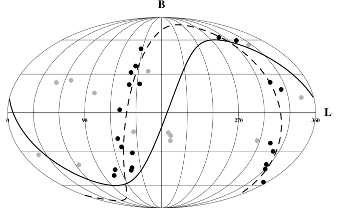
Fig. 6: The scatter distribution for aphelia directions of $17th$ Catalogue class 1A OOC comets having a binding energy parameter, $x\equiv 10^{6}$ AU/$A$, in the interval $30<x<60$ and tidal characteristic $S$=-1. Solid curve: ecliptic plane. Dashed curve: best fit perturber plane with $i=103^{\circ},\;\Omega=319^{\circ}$. Black dots: aphelia directions within a band of width $\pm 9.6^{\circ}$ covering 1/6 of the celestial sphere and centered on the best fit great circle path. Gray dots: exterior to the band.

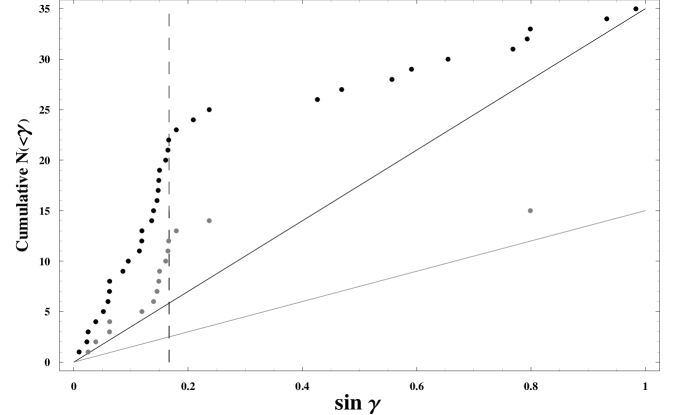
Fig. 7: The cumulative distribution of the number of major axes of class 1A OOC comets having $30<x<60$ and $S=-1$ that fall within an annular band of solid angle $4\pi\sin\gamma$ centered on the best fit great circle $i=103^{\circ},\;\Omega=319^{\circ}$. Black: $17th$ Catalogue data. Gray: 11th Catalogue data. Solid lines are for random distributions. Dashed line indicates annular band of width $\pm 9.6^{\circ}$ which includes 1/6 of the celestial sphere.

In Fig. 6 we illustrate the scatter of aphelia directions in galactic coordinates with the best fit great circle arc ($i=103^{\circ},\;\Omega=319^{\circ}$) shown. The data illustrated is for the $17th$ Catalogue with $30<x<60$ and $S=-1$. Major axes are distinguished if they are within the $\pm 9.6^{\circ}$ band. The distribution of major axes around the great circle arc indicates comparable numbers in each of the 4 quadrants. This is inconsistent with an overpopulation produced by a weak stellar perturbation which produces an overpopulated arc $<150^{\circ}$ in length (Matese and Lissauer (2002)). In Fig. 7 we show the cumulative number of major axes interior to the solid angle, $4\pi\sin\gamma$, subtended by a band of width $\pm\gamma$ centered on the best fit great circle. For comparison, results are shown for the $17th$ Catalogue data as well as the corresponding 11th Catalogue data.

Using an approach that ignores the characteristic $S$, Murray (1999) has argued for a solar companion that is the source of a impulsed observed OOC population with $40\leq x\leq 100$ whose axes are concentrated along a great circle that is different from that found here. He found that all class 1A comets in the 10th Cometary Catalogue had axes within a $\pm 30^{\circ}$ band. His point is essentially that all of these observed comets must have been injected into the loss cylinder by an impulse of a bound companion. We have taken the $17th$ Catalogue data and considered all 1A ($40\leq x\leq 100$) comets that also were included in Murray’s paper which analyzed $10th$ Catalogue data. A fit to the original data is found to agree with Murray’s result, a best fit companion orbit plane with a galactic inclination of $i=37^{\circ}$ and galactic ascending node of $\Omega=175^{\circ}$ that includes all 12 $10th$ Catalogue axes within a band of $\pm 30^{\circ}$ which encloses 1/2 of the celestial sphere. When we repeat the fit with the same band orientation and width we find that 10 of 25 additional comets in the $17th$ Catalogue are enclosed. The concentration originally perceived is seen to have disappeared.

4.2 IR observational limits on the companion’s mass and distance

The absence of detection in the IRAS and 2mass data bases place limits on the range of possible masses and present distances of the proposed companion. For relevant values the 2mass limits are not very restrictive. Assuming a J-band detection magnitude limit of 16 and theoretical models of a 4.5 Gyr old 2-10 M_J object (Burrows et al. (2003)), we find that the mass would have to be greater than 7 (10)M_J and closer than $6000\;(25,000)$ AU for a possible 2mass identification.

For Jovian masses, the strongest current limits on distance are found from the IRAS Point Source and Faint Source Catalogs. We have performed a non-parallax search of both IRAS catalogs using the VizieR Service (http://vizier.u-strasbg.fr/cgi-bin/VizieR). The search was based on the theoretical models of Burrows et al. (2003). Search criteria included rejection of previously identified point sources, a PSC 12 $\mu$m flux greater than 1 Jy and a FSC flux greater than 0.3 Jy. The latter value is based on a completion limit of 100% (Moshir et al. 1992). Only flux quality class 1 sources were included. We further required that there be no bright optical or 2mass candidates within the 4$\sigma$ error limits and that the absolute value of the galactic latitude be greater than 10 degrees, as required for sources to appear in the FSC. Distant IR galaxies were excluded by requiring the 25 $\mu$m flux to be greater than the 60 $\mu$m flux. The PSC search yielded a single candidate, 07144+5206, with galactic coordinates B = 25^o and L = 165^o, not far from the great circle band. The 12 and 25 $\mu$m band flux (0.8 Jy and 0.5 Jy) of this source is consistent with a $\approx$ 6 M_J mass at $\approx 6000$ AU. However, the FSC, which is the definitive catalog for faint sources, associated this PSC source with another source located 80 arc sec away. This position corresponded to an extremely bright (J=6) 2mass source. The negative IRAS search results suggest that an object of mass 2 (5) $\rm{M_{J}}$ must have a current distance $r\geq 2000\;(10,000)$ AU, respectively.

4.3 Dynamical inferences of other perturber properties

Although the orbit normal of the putative companion is tightly constrained, other properties are less so. If it exists, a solar companion most likely formed in a wide-binary orbit. The near-uniform distribution of the overpopulation around the great circle suggests that any putative companion is likely to have a present orbit that is more nearly circular than parabolic (${e_{p}}^{2}<0.5$). The near-circular implication cannot remain true over the solar system lifetime since the eccentricity and inclination osculate significantly due to the tide. Further, the semimajor axis will be affected by stellar impulses over these timescales.

The implication that ${e_{p}}^{2}<0.5$, is in fact, consistent with the present galactic inclination of the perturber inferred here, $i\approx 103^{\circ}$. This follows from the near-conservation of the $\mathbf{\hat{z}}$ component of galactic angular momentum of objects in the IOC and OOC in the intervals between strong stellar impulses, $H_{z}\propto\ b\;\cos i\approx{\rm constant}.$ Since the present value of $|\cos 103^{\circ}|\approx 0.22$ is at the low end of a random distribution, $0\leq|\cos i|\leq 1$, a larger primordial value of $|\cos i|$ implies that the present value of $e_{p}$ is reduced from its primordial value.

Fig. 8: Integrating back in time for 4.6 Gy the osculating orbit of a putative companion with present ($t\equiv 0$) galactic orbital elements $i(0)=103^{\circ},\;\Omega(0)=319^{\circ},\;\omega(0)=0,\;a=15,000{\rm AU},\;e_{p}(0)=0.5,\;q(0)=7500$ AU assuming unchanging galactic environment and neglecting impulsive perturbations. Shown are the perihelion distance, $q(t)$, and the semiminor axis, $b(t)$, along with the galactic and ecliptic inclinations, $i(t)$ and $i_{e}(t)$.

In Fig. 8 we show a representative time dependent companion orbit assuming present ($t_{o}\equiv 0$) galactic orbital elements $i=103^{\circ},\;\Omega=319^{\circ},\;\omega=0,\;a=15,000{\rm AU}$ and $e_{p}$ = 0.5. We integrate back in time assuming an unchanging galactic environment and neglecting impulsive perturbations, both of which cannot be ignored for more reliable results. The purpose of the calculation is to demonstrate that significant changes in the eccentricity and inclination occur over the solar system lifetime for a companion with $a>10^{4}$AU.

There is no evidence of overpopulation within the perceived band of OOC or IOC comets with $60<x$ where $|\mathbf{\Delta H_{tide}}|<|\mathbf{\Delta H_{min}}|$. Here we must distinguish two subpopulations of discernable comets with $60<x$ (assuming negligible errors in $x$), (i) comets that have been directly injected from beyond the loss cylinder by the perturbation and are making their first orbit as discernable comets, or, (ii) comets that are daughters of $x<60$ comets which had a previous perihelion passage well inside the loss cylinder. The latter is the commonly accepted pathway for producing discernable IOC comets, but requires an ad hoc imposition of a fading mechanism (Wiegert and Tremaine (1999)) to explain the relative numbers of observed IOC and OOC comets.

For a comet major axis inclined to the perturber orbit plane by an angle $\gamma$ $\;\mathbf{|\Delta H_{pert}|_{max}}$ varies approximately as $1/\gamma$, and the cross section for scattering comets varies approximately as $\gamma^{2}$. Thus one expects that a perturber in a crossing orbit with some $60<x$ comets would produce a narrower band of detectable flux perturbed with $|\mathbf{\Delta H_{pert}}|>|\mathbf{\Delta H_{min}}|$. The absence of such a directly impulsed population (i) is not inconsistent with the notion that the depletion rate of this population in crossing orbits within the great circle band by the perturber would be larger than the rate of refilling of the band phase space by the galactic tide.

More difficult to explain is the absence of an enhanced daughter population (ii) in the perceived band. A possible explanation is that the reduced impulse/reflex interaction can remove daughters by a random-walk of their perihelia from inside the discernable zone leading to ejection over one or more subsequent orbits. A direct numerical integration, including a putative companion, of the type done by Kaib and Quinn (2009) is needed to clarify this matter. This scenario would require $a$ to be at the small end of the allowed range.

Setting the critical perturbation for $\gamma=9.6^{\circ}$ equal to the minimum change required to enter the discernable zone, Eq.  5 yields

$$\mathbf{|\Delta H_{pert}|_{crit}}=\sqrt{\mu_{\odot}\;a}\;\frac{\mu_{p}}{\mu_{\odot}}\;\mathbf{|\widehat{Q}\times I|_{crit}}\equiv\mathbf{|\Delta H_{min}|}\approx\sqrt{\mu_{\odot}\;5.4{\rm{AU}}}.$$ (7)

This provides a means of estimating the perturber properties needed to weakly impulse the OOC comet population and assist the tide in making a comet with $30<x<60$ discernable. Here $\mathbf{|\widehat{Q}\times I|_{crit}}$ is taken to be $\simeq$ the peak values of $\mathbf{|\widehat{Q}\times I|}$ sampled over all orientaions of $\mathbf{\widehat{Q}}$ that are inclined to the great circle by an angle $\gamma=\pm 9.6^{\circ}$

$$\frac{M_{p}}{{\rm M_{\odot}}}\;\sqrt{\frac{a}{5.4{\rm AU}}}\;\mathbf{|\widehat{Q}\times I|_{crit}}=1.$$ (8)

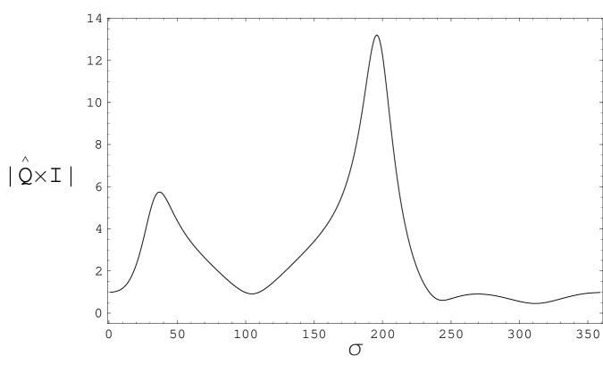
Fig. 9: An example case showing the single-orbit impulse strength $\mathbf{|\widehat{Q}\times I|}$ for comets with $A=22,000$ AU and $\mathbf{\widehat{Q}}$ inclined to the perturber plane by $\gamma=9.6^{\circ}$. The positions $\sigma=0(180^{\circ})$ correspond to comet orientation $\mathbf{\widehat{Q}}$ closest to the perturber perihelion (aphelion). Perturber parameters are $a=15,000$ AU, $e_{p}=0.5$, and $f_{o}=215^{\circ}$, the present true anomaly of the perturber.

In Fig. 9 we show an illustrative plot of $\mathbf{|\widehat{Q}\times I|}$ for perturber parameters $a=15,000{\rm AU},\;e_{p}=0.5,\;f_{o}=215^{\circ}$ and comet $A=22,000{\rm AU}$. A set of major axis orientations, $\mathbf{\widehat{Q}}$, are considered which are all inclined along a conical surface at an angle $\gamma=9.6^{\circ}$ to the perturber plane. The specific orientation $\sigma=180^{\circ}$ corresponds to the case where $\mathbf{\widehat{Q}}$ is closest to the perturber aphelion direction. The arbitrarily chosen present location of the companion is $f_{o}=215^{\circ}$ so that it has recently passed aphelion. Two peaks are shown corresponding to the two comet axes $\mathbf{\widehat{Q}}$ that are most strongly perturbed on the way out and on the way in during the prior cometary orbit. The peak at $\sigma=195^{\circ}$ locates the perturber position when comets were perturbed on their inward leg. The ratio of the comet/perturber periods is $\approx$1.8 in this case and the second peak at $\sigma=35^{\circ}$, corresponds to the outward leg when the perturber was on its previous orbit. The importance of the reflex term can be gauged from the background contribution. In general the peak corresponding to the inward comet leg will slightly lag the present perturber position if the perturber is presently more nearly at aphelion. The second peak corresponding to the outward leg will, in general, tend to be randomly positioned relative to the inward peak if $A>a$. Each peak contains comet axes $\mathbf{\widehat{Q}}$ that have angular momentum component impulses that both aid the tide and oppose the tide.

The results shown are typical for all $e_{p}<0.5,\;90^{\circ}<f_{o}<270^{\circ}$ when $10,000{\rm AU}<a<30,000$AU. The exceptions include the less likely cases when the perturbations on both the outward and inward legs of a comet orbit find the perturber at the same general location $f\approx\sigma$ creating a larger net impulse. We shall adopt a typical value of $\mathbf{|\widehat{Q}\times I|_{crit}}\approx 6-12$ for all possible orbit parameters above. Smaller values in this range typically occur for smaller values of $a$ which have higher relative velocities at orbit crossing. Another aspect of the variation is that the small reflex term can add or subtract from the direct impulse term.

Inserting $M_{p}=5{\rm M_{J}}$ into Eq.  8 we obtain $a\leq 6000$ AU. Assuming ${e_{p}}^{2}<0.5$, this is marginally inconsistent with IRAS observational limits. Smaller masses should not conflict with IRAS. Thus we adopt an approximate range of perturber parameters $1{\rm M_{J}}<M_{p}<2{\rm M_{J}}$ for $a\approx 30,000\rm{AU}$ extending to $2{\rm M_{J}}<M_{p}<4{\rm M_{J}}$ for $a\approx 10,000\rm{AU}$. This companion mass range is consistent with the minimum Jeans mass (1 - 7) M_J as variously calculated (Whitworth (2006), Low and Lynden-Bell (1976)).

A solar companion remains a viable option (Matese et al. (1999); Horner and Evans (2002)). In addition, we find that an $\approx 4\;{{\rm M_{J}}}$ companion in an orbit such as that shown in Fig. 8 would be capable of adiabatically detaching a scattered disk EKBO, producing an object with orbital characteristics similar to Sedna (Matese et al. (2006); Gomes et al. (2006)). Allowing for the possibility that the perturber was more tightly bound primordially, smaller masses are then allowed. It may also be possible to explain the misalignment of the invariable plane with the solar spin axis (Gomes et al. (2006)) if the putative companion was more tightly bound primordially. Such a companion would have a temperature of $\approx 200$ K (Burrows et al. (2003)) and will be easily seen by the Wide-field Infrared Survey Explorer ((2007)) recently launched. Gaia, which will use astrometric microlensing, may also be able to detect the putative companion and will be launched in 2011 (Gaudi and Bloom (2005)).

Matese and Lissauer (2002) investigated the frequency of weak stellar showers as well as the patterns of discernable OOC comet orbital elements. They found that stellar showers that produce a $\geq 20\%$ peak enhancement in the background tidal flux occur with a frequency of approximately once every 15 Myr. The half-maximum duration is $\approx 2$ Myr. Thus it is only moderately unlikely that we are presently in a weak stellar shower of this magnitude.

Flux enhancements of this magnitude were found to extend over an angular arc $\approx 150^{\circ}$ and have a full-width half-max of $\approx 50^{\circ}$. Weak stellar impulses never extend over a larger arc. More simply put, to get the same stellar-induced flux enhancement as inferred from the data here, the enhanced region will have an extent that is $\approx$ half as long and $\approx$ twice as wide as that observed. Of course one must consider the possible alignment of two weaker coincident stellar impulses (or a single weaker statistical anomaly and a coincident single weaker stellar impulse) that happen to line up on opposite hemispheres. These will be improbable. For example, suppose we assume that there will always be two weak stellar impulses enhancing the observed background tidal flux, each with half the observed enhancement. The probability that both stellar orbit planes will be aligned to within $\pm 9.6^{\circ}$ is 0.014.

4.4 A Monte Carlo test for the likelihood of the conjecture.

For each of the three data sets discussed above we perform a variation of the Monte Carlo test done elsewhere (Horner and Evans (2002)) which considered the original conjecture. Each comet in the data maintains its measured value of $B$, but is randomly assigned a value for $L$. The best fit analysis is performed to find the orientation of the great circle band of width $\pm 9.6^{\circ}$ which maximizes the number of major axes interior to the band, just as was done for the real data. We then record that number, $n$. Repeating the process for each data set $5000\times$ we can find the Monte Carlo probability that $\geq n$ major axes would fall in the band if, in fact, $L$ was truly random. Results are given in Table 1. As an example, for the $17th$ Catalogue data, when we randomize $L$ for the 35 comets we found an unconstrained (i.e. randomly oriented) band of width $\pm 9.6^{\circ}$ which maximized the number of major axes contained in the band at 18 or more in 30 cases of the $5000$ tested.

Table 1: Monte Carlo probability ${}^{\mathcal{E}}\mathcal{P}_{MC}(\geq n)$ for Catalogue data set $\mathcal{E}$

$\mathcal{E}$	$n_{max}$	$n\rightarrow$	10	11	12	13
$11th$	15		0.018	0.0020	0.0002	$<$0.0002
$17th-11th$	20		0.24	0.078	0.015	0.0014
		$n\rightarrow$	18	19	20	21
$17th$	35		0.0060	0.0018	0.0008	$<$0.0002

A preliminary discussion of the persistence of the enhancement is as follows. The Monte Carlo probability, ${}^{11th}\mathcal{P}_{MC}(\geq 10)=0.018$ for the original data set is superficially significant. The solid angle over which this occurs can be seen in Fig. 5 to be $<2\%$ of the celestial sphere. As many as $n=13$ of 15 axes can be found in a band for the actual data. Although the Monte Carlo analysis for the $17th-11th$ Catalogue data set is, in itself, not significant since at most 11 comets appear in a band for the actual data and ${}^{17th-11th}\mathcal{P}_{MC}(\geq 10)=0.24$, the fact that the cone of normal directions that maximizes the counts for this data set overlaps with the cone that maximizes the $11th$ Catalogue data set is significant. To properly gauge this significance we discuss a Bayesian analysis of the likelihood of the present conjecture.

4.5 Bayesian inference

The anomalous comet data discussed above can be explained by the putative companion. We now wish to compare this hypothesis with other hypotheses that might also explain the data. The most obvious alternative explanation is that the anomaly is entirely a statistical fluke. The other dynamical explanation is that of a weak stellar shower assisted by the galactic tide. Arguments against this possibility have been given earlier and in the following analysis we assume the probability of a shower explanation is negligible.

We consider the hypothesis, $\mathcal{H}$, that the there exists a Jovian mass solar companion orbiting in the Oort cloud with parameters in the previously discussed ranges that are allowed on the basis of IRAS/2mass observations. The null hypothesis, $\mathcal{\neg H}$, is that no such object exists. $\mathcal{E}$ constitutes the evidence considered, the $30<x<60,\;S=-1$ data sets described in Fig. 5 and Table 1. The a priori relative probability of hypothesis $\mathcal{H}$, before we consider evidence $\mathcal{E}$, is symbolically defined as ${\mathcal{P}(\mathcal{H})}/{\mathcal{P}(\neg\mathcal{H})}$.

IRAS and 2mass observational constraints prohibit present locations $r<2000:\;\;10,000:\;\;25,000$ AU for $M_{p}=2:\;5:\;10\;{\rm M_{J}}$ respectively. Dynamical constraints previously discussed suggest a companion mass in the range $M_{p}\approx$ 1 - 4 M_J and semimajor axis in the range $a\approx 30,000-10,000$ AU, respectively. Qualitatively ${\mathcal{P}(\mathcal{H})}/{\mathcal{P}(\neg\mathcal{H})}$ is the ratio of the specified companion parameter space area ($M_{p},a$) to the complementary, non-IRAS(2mass)-excluded parameter space area. Next we try to roughly estimate this from the non-Catalogue evidence.

We assume that there is a certainty that the sun has an as-yet-to-be-discovered maximum mass companion with mass between ${\rm M_{Pluto}}\longleftrightarrow 20{\rm M_{J}}$, the upper limit being fixed by IRAS/2mass observations. Zuckerman and Song (2008) give a mass distribution for brown dwarfs down to 13 ${\rm M_{J}}$ of $dN/dM\propto M^{-1.2}$. It might be assumed that this power law roughly holds down to the minimum Jeans mass limit of 1 - 4 ${\rm M_{J}}$ (Whitworth (2006)) but the mass distribution below 1 ${\rm M_{J}}$ is completely unknown. For simplicity we assume $dN/dM\propto M^{-1}$ over the entire mass range.

Next we estimate the probability distribution in semimajor axis for this companion, assumed to be in the interval $10^{2}\longleftrightarrow 10^{5}$ AU. We base this estimate on the known distribution of semimajor axes of wide binary stars. At least 2/3 of solar type stars in the field reside in binary or multiple star systems (Duquennoy and Mayor (1991)). The fraction of these systems which have semimajor axes $a\geq$ 1000 AU (wide binaries) is $\approx$ 15% (Kouwenhoven et al. (2010), Duquennoy and Mayor (1991) ), and includes periods up to 30 Myr. The origin of these wide binaries may be capture during cluster dissolution (Kouwenhoven et al. (2010)). For large semimajor axes the observed distribution is well approximated by $(dN/da)\propto a^{-1}$ and we adopt this power law for all masses over the entire interval of $a$.

The simplifying assumptions we have made are equivalent to assuming a uniform probability distribution over the entire parameter space ($M_{p},a$) under consideration

$$\frac{d^{2}N}{d\log M_{p}\;d\log a}={\rm constant}.$$

Thus the combined probability that the sun has a companion of mass 1 - 4 M_J with semimajor axis 30,000 - 10,000 AU is simply the ratio of this parameter area to the entire area after the IRAS constraint has been utilized. In the following Bayesian analysis we use this value for the a priori probability ratio, ${\mathcal{P}(\mathcal{H})}/{\mathcal{P}(\neg\mathcal{H})}\approx 0.01$.

The likelihood ratio of $\mathcal{H}$ given $\mathcal{E}$ is

$$\Lambda_{\mathcal{H}:\mathcal{E}}\equiv\frac{\mathcal{P}(\mathcal{E}|\mathcal{H})}{\mathcal{P}(\mathcal{E}|\neg\mathcal{H})}$$ (9)

where $\mathcal{P}(\mathcal{E}|\mathcal{H})$ is the conditional probability of evidence $\mathcal{E}$ if hypothesis $\mathcal{H}$ is true. More meaningful is the a posteriori relative probability, a product of the a priori relative probability and the likelihood ratio

$$\frac{\mathcal{P}(\mathcal{H}|\mathcal{E})}{\mathcal{P}(\neg\mathcal{H}|\mathcal{E})}\equiv\Lambda_{\mathcal{H}:\mathcal{E}}\;\frac{\mathcal{P}(\mathcal{H})}{\mathcal{P}(\neg\mathcal{H})}.$$ (10)

4.5.1 Analysis of the $17th$ Catalogue alone

In this case we adopt the Monte Carlo results of Table 1 for the likelihood ratio

$$\Lambda_{\mathcal{H}:\emph{17th}}=\frac{1}{{{}^{17th}}\mathcal{P}_{MC}(\geq n)}$$

to obtain an a posteriori probability ratio

$$\frac{\mathcal{P}(\mathcal{H}|17th)}{\mathcal{P}(\neg\mathcal{H}|17th)}=\frac{0.01}{{{}^{17th}}\mathcal{P}_{MC}(\geq n)}.$$

Inserting the results from Table 1 the a posteriori relative probability ratio is $\approx 10$ for $n=20$ with corresponding changes for other values of $n$.

4.5.2 Separate analyses of the $11th$ and $17th-11th$ subsets

For $\mathcal{E}=\emph{11th}$ we make the same assumption about the a priori relative probability to obtain

$$\frac{\mathcal{P}(\mathcal{H}|11th)}{\mathcal{P}(\neg\mathcal{H}|11th)}=\frac{0.01}{{{}^{11th}}\mathcal{P}_{MC}(\geq n)}$$

from which we obtain $\approx 0.5$ for $n=10$ with corresponding changes for other values of $n$.

For $\mathcal{E}=\emph{17th-11th}$ we must take into account that the 11th Catalogue data defined a specific cone of directions in space. In this case we adjust our likelihood ratio estimate of the Monte Carlo results of Table 1 by the probability that the cones of the orbit normals containing maximum counts would overlap which is $\approx 0.02$ to obtain an a posteriori probability ratio

$$\frac{\mathcal{P}(\mathcal{H}|17th-11th)}{\mathcal{P}(\neg\mathcal{H}|17th-11th)}=\frac{0.01}{0.02\left[\;{}^{17th-11th}\mathcal{P}_{MC}(\geq n)\right]}$$

from which we obtain results of $\approx 2$ for $n=10$ with corresponding changes for other values of $n$.

An alternative approach is to allow our $11th$ Catalogue inference to adjust the a priori relative probability for $\mathcal{E}=17th-11th$ (if the cones overlap) to equal the a posteriori result for $\mathcal{E}=11th$

$$\frac{\mathcal{P}(\mathcal{H}|17th-11th)}{\mathcal{P}(\neg\mathcal{H}|17th-11th)}=\frac{0.5}{{}^{17th-11th}\mathcal{P}_{MC}(\geq n)}$$

which also yields $\approx 2$ for $n=10$.

All of these inferences can be scaled if a value of the a priori relative probability is chosen different from 0.01 based on other evidence than considered here (IRAS/2mass observational limits and stellar/brown dwarf mass and semimajor axis distributions). Specifically this value might be increased if one believed that the Jovian companion hypothesis, $\mathcal{H}$, provides a plausible explanation for producing Sedna, and it would be substantially reduced if one believed that the hypothesis is incompatible with the absence of an enhanced IOC daughter population along the perceived arc.

We can estimate the size of the impulsive enhancement in the present data for 102 class 1A comets as follows. Although only 13 of 35 comets lie outside of the $\pm 9.6^{\circ}$ band for our best fit, statistically significant results obtain if as many as 17 of 35 were outside the band. So, conservatively, we would expect $\approx 3$ inside the band if there were no impulsively enhanced component. The excess of $\approx 15-19$ inside the band is $\approx 20\%$ of the complementary number of 87-83 for the complete 1A data listed in the Appendix. The same number can be obtained by extrapolating back to zero the large $\sin\gamma$ portion of the cumulative curve in Fig. 6.

5 Summary and conclusions

We have described how the dynamics of a dominant galactic tidal interaction, weakly aided by an impulsive perturbation, predicts specific properties for observed distributions of the galactic orbital elements of outer Oort cloud comets. These subtle predictions have been found to be manifest in high-quality observational data at statistically significant levels, suggesting that the observed OOC comet population contains an $\approx 20\%$ impulsively produced excess. The extent of the enhanced arc is inconsistent with a weak stellar impulse, but is consistent with a Jovian mass solar companion orbiting in the OOC. A putative companion with these properties may also be capable of producing detached Kuiper Belt objects such as Sedna and has been given the name Tyche. Tyche could have significantly depleted the inner Oort cloud over the solar system lifetime requiring a corresponding increase in the inferred primordial Oort cloud population. A substantive difficulty with the Tyche conjecture is the absence of a corresponding excess in the presumed IOC daughter population.

ACKNOWLEDGMENTS

The authors thank Jack J. Lissauer for his continuing interest and for his contributions to this research.

Appendix

Table 2:             Class 1A OOC orbital elements. All angles are in degrees.

Comet name	$x$	$S$	$q$(AU)	$B$	$L$	$\alpha$	$\gamma$
C/1996 J1-A(B)	-510(-1)	-1	1.2978	15.9	202.6	55.0	51.13
C/1996 E1	-42	1	1.3590	-22.6	304.3	319.2	18.39
C/1942 C2	-34	1	4.1134	-24.5	18.8	335.2	42.27
C/1946 C1	-13	1	1.7241	-60.3	313.1	276.7	14.17
C/2005 B1	-13	1	3.2049	-17.6	82.6	12.7	38.28
C/1946 U1	-1	1	2.4077	49.0	347.2	255.0	28.13
C/1997 BA6	0	-1	3.4364	27.7	123.0	52.9	20.05
C/1993 Q1	3	1	0.9673	41.2	112.7	174.6	28.22
C/2005 K1	7	1	3.6929	-17.3	227.4	312.1	85.45
C/2003 T3	10	1	1.4811	25.5	293.6	148.9	16.25
C/2006 L2	10	-1	1.9939	-50.0	225.1	98.2	52.89
C/1974 V1	11	-1	6.0189	28.0	308.9	63.1	2.61
C/1988 B1	13	-1	5.0308	-47.6	316.3	122.1	11.37
C/2006 K1	13	1	4.4255	66.1	56.2	247.3	36.69
C/2004 X3	14	1	4.4023	-36.8	80.9	24.1	31.90
C/2005 E2	14	1	1.5196	42.0	312.6	134.6	3.99
C/2006 OF2	15	1	2.4314	10.5	322.5	133.0	5.75

Comet name	$x$	$S$	$q$(AU)	$B$	$L$	$\alpha$	$\gamma$
C/1991 F2	16	-1	1.5177	29.7	90.0	345.1	48.65
C/2005 G1	16	-1	4.9607	-55.3	297.9	100.6	22.60
C/1916 G1	17	-1	1.6864	17.9	225.9	30.1	58.95
C/1956 F1-A	17	1	4.4473	-25.4	180.0	62.1	42.33
C/1944 K2	18	-1	2.2259	-31.8	124.3	159.3	5.25
C/2007 O1	18	-1	2.8767	2.1	197.3	7.6	55.06
C/1935 Q1	19	1	4.0434	11.8	248.0	115.3	58.81
C/1999 J2	19	-1	7.1098	-49.9	234.4	259.3	52.80
C/1973 E1	20	-1	0.1424	17.0	207.3	46.3	53.15
C/1984 W2	20	1	4.0002	33.1	79.5	101.0	55.69
C/2001 C1	20	1	5.1046	-8.3	135.0	344.1	2.02
C/2004 P1	20	-1	6.0141	20.2	208.7	63.7	51.26
C/1922 U1	21	-1	2.2588	16.3	270.6	52.4	39.46
C/1997 A1	21	1	3.1572	-19.9	352.3	306.7	25.22
C/2003 K4	23	1	1.0236	-46.8	104.3	307.2	12.49
C/2005 Q1	23	-1	6.4084	-8.8	321.7	258.1	0.65
C/1947 S1	24	1	0.7481	10.9	185.4	170.2	40.61
C/1978 H1	24	1	1.1365	-20.7	124.4	30.2	8.65
C/1999 K5	24	-1	3.2554	34.1	129.8	271.8	14.81
C/2001 G1	24	-1	8.2356	-46.8	113.6	118.9	7.02
C/2006 HW51	25	1	2.2656	-35.4	162.3	83.4	26.39
C/1914 M1	27	-1	3.7468	-1.4	200.9	100.9	59.81
C/1980 E1	27	1	3.3639	-18.2	177.0	29.9	39.78
C/2004 YJ35	27	-1	1.7812	-38.2	346.3	122.2	12.23

Comet name	$x$	$S$	$q$(AU)	$B$	$L$	$\alpha$	$\gamma$
C/1992 J1	28	1	3.0070	-43.8	316.9	0.3	10.47
C/1913 Y1	29	-1	1.1045	-52.4	283.0	237.4	31.83
C/1987 W3	29	-1	3.3328	64.7	333.5	62.5	17.92
C/2001 K5	29	1	5.1843	-30.3	223.1	78.8	71.80
C/1989 X1	32	-1	0.3498	-41.0	325.6	218.0	3.57
C/1978 A1	33	-1	5.6064	-31.4	142.3	167.8	9.48
C/1993 K1	33	-1	4.8493	2.3	130.9	347.4	8.38
C/1948 E1	34	1	2.1071	-38.6	250.2	83.2	58.25
C/1948 T1	34	-1	3.2611	17.9	324.0	306.9	8.63
C/2006 Q1	34	-1	2.7636	-45.5	112.2	134.0	8.48
C/1925 F1	35	1	4.1808	-40.9	65.6	327.8	33.96
C/2002 J4	35	-1	3.6338	32.4	162.6	342.6	12.07
C/1974 F1	36	-1	3.0115	21.7	140.3	10.7	3.59
C/2003 S3	36	-1	8.1294	11.6	345.3	351.9	27.95
C/2004 B1	36	1	1.6019	27.7	167.1	138.4	17.55
C/1950 K1	37	-1	2.5723	-43.8	137.7	269.9	8.02
C/1999 U4	37	-1	4.9153	-30.2	322.6	183.8	3.42
C/2006 E1	37	-1	6.0406	31.4	140.5	290.6	21.24
C/2006 P1	37	1	0.1707	-5.0	342.2	72.9	5.47
C/1999 F1	38	-1	5.7869	15.2	99.7	341.0	68.86
C/1999 U1	38	-1	4.1376	25.1	67.4	291.1	40.91
C/2000 CT54	38	-1	3.1561	36.7	145.1	8.0	2.96
C/2002 L9	38	-1	7.0330	51.6	147.6	292.5	4.93
C/1954 Y1	39	-1	4.0769	-23.5	314.1	232.3	9.55

Comet name	$x$	$S$	$q$(AU)	$B$	$L$	$\alpha$	$\gamma$
C/1925 G1	40	1	1.1095	10.5	238.3	151.2	64.77
C/1997 J2	40	1	3.0511	-0.5	261.1	332.6	55.83
C/1954 O2	42	1	3.8699	-18.4	336.4	53.3	11.82
C/1979 M3	42	1	4.6869	14.1	207.0	126.6	55.24
C/2000 K1	42	-1	6.2761	-21.6	190.7	144.5	52.50
C/2006 S3	42	-1	5.1309	-15.3	188.0	219.4	50.21
C/1946 P1	44	-1	1.1361	-20.0	126.6	108.7	6.85
C/1999 Y1	44	-1	3.0912	62.7	289.2	326.2	1.31
C/2000 A1	44	-1	9.7431	-33.0	19.7	171.9	36.22
C/2005 EL173	44	-1	3.8863	23.3	50.4	350.5	79.60
C/1932 M2	45	-1	2.3136	-14.6	146.5	172.1	10.33
C/1987 H1	46	-1	5.4575	-17.6	190.9	161.4	53.02
C/1888 R1	48	-1	1.8149	59.5	313.7	289.0	8.54
C/1983 O1	48	-1	3.3179	55.2	324.4	355.4	13.71
C/1973 A1	49	-1	2.5111	-50.7	106.2	220.9	9.24
C/1989 Y1	49	1	1.5692	-6.1	328.9	96.2	8.22
C/2007 D1	50	-1	8.7936	-41.3	64.4	157.8	33.83
C/2003 WT42	51	-1	5.1909	-56.8	353.7	171.0	6.59
C/2000 O1	52	-1	5.9217	23.5	313.8	286.2	25.23
C/2000 SV74	52	-1	3.5417	-21.5	296.7	193.5	0.53
C/1999 F2	54	-1	4.7188	-46.0	135.3	112.9	6.83
C/1999 S2	56	-1	6.4662	22.2	153.2	322.9	7.83
C/2006 K3	56	1	2.5015	46.6	22.7	261.9	49.79

Comet name	$x$	$S$	$q$(AU)	$B$	$L$	$\alpha$	$\gamma$
C/1976 D2	59	1	6.8807	-44.5	120.9	315.8	3.36
C/1987 F1	59	-1	3.6246	-26.5	129.8	186.4	2.20
C/1993 F1	59	-1	5.9005	-45.0	330.2	213.7	1.44
C/2002 J5	60	-1	5.7268	-33.0	240.2	157.1	67.57
C/2005 L3	60	-1	5.5933	-30.3	203.9	169.6	61.07
C/2000 Y1	61	-1	7.9748	28.0	350.3	8.5	33.52
C/1999 H3	65	-1	3.5009	-50.1	250.1	167.3	49.12
C/1898 L1	68	-1	1.7016	28.3	143.8	315.4	2.01
C/1999 N4	68	-1	5.5047	-23.3	200.6	204.1	61.14
C/1972 L1	69	1	4.2757	-40.3	235.4	66.6	62.09
C/2007 JA21	69	-1	5.3682	-31.4	272.5	247.5	46.07
C/1958 R1	76	-1	1.6282	-18.4	307.6	133.4	14.74
C/1955 G1	82	-1	4.4957	-29.8	233.2	168.5	72.73
C/2005 A1-A	94	-1	0.9069	29.4	113.9	12.6	28.06

References

- Burrows et al. ( 2003) Burrows, A., D. Sudarsky, and J. J. Lunine 2003. Beyond the T dwarfs: Theoretical spectra, colors and detectability of the coolest brown dwarfs. burrows/evolution3.html)AP. J. 596, 587-596.
- Davis et al. ( 1984) Davis, P. Hut, and R. Muller 1984. Extinction of species by periodic comet showers. Nature 308, 715-717. 308, 715 717. Nature
- Delsemme ( 1987) Delsemme, A. H. 1987. Galactic tides affect the Oort cloud: an observational confirmation. Astron. Astrophys. 187, 913-918.
- Duquennoy and Mayor ( 1991) Duquennoy, A. and M. Mayor 1991. Multiplicity among solar-type stars in the solar neighborhood: II. Distribution of the orbital elements in an unbiased sample.Astron. Astrophys. 248, 485-524.
- Fernandez ( 1981) Fernandez, J. 1981. New and evolved comets in the Solar System. Astron. Astrophys. 96, 26-35.
- Gaudi and Bloom ( 2005) Gaudi, B. S., and J. S. Bloom. 2005. Astrometric microlensing constraints on a massive body in the outer solar syatem with Gaia. Ap. J. 635, 711-717.
- Gomes et al. ( 2006) Gomes, R. S., J. J. Matese, and J. J. Lissauer 2006. A distant planetary-mass solar companion may have produced distant detached objects. Icarus 184, 589-601.
- Heisler and Tremaine ( 1986) Heisler, J., and S. Tremaine 1986. Influence of the galactic tidal field on the Oort cloud. Icarus 65, 13-26.
- Horner and Evans ( 2002) Horner, J., and N. W. Evans 2002. Biases in cometary Cataogues and Planet X. Mon. Not. R. Astron. Soc. 335, 641-654.
- Kaib and Quinn ( 2009) Kaib, N. A., and T. Quinn 2009. Reassessing the source of long-period comets. Science 325, 1234-1236.
- Kirkpatrick and Wright ( 2010) Kirpatrick, D. and N. Wright 2010. (quoted in) Sun’s Nemesis pelted Earth with comets, study suggests. Space.com/scienceastronomy/nemesis-comets-earth-am-100311.html.
- Kouwenhoven et al. ( 2010) Kouwenhoven, M. B. N., S. P. Goodwin, R. J. Parker, M. B. Davies, D. Malmberg, and P. Kroupa 2010. The formation of very wide binaries during the star cluster dissolution phase. arXiv:1001.3969V1[astro-ph.GA]
- Kresák ( 1992) Kresák, L. 1992. Are there any comets coming from interstellar space? Astron. Astrophys. 259, 682-691.
- Królikowska ( 2006) Królikowska, M. 2006. Non-gravitational effects in long-period comets and the size of the Oort cloud. Acta Astronomica 56, 385-412.
- Low and Lynden-Bell ( 1976) Low, C. and D. Lynden-Bell 1976. The minimum Jeans mass when fragmentation must stop. Mon. Not. R. Astr. Soc., 176, 367-390.
- Marsden et al. ( 1978) Marsden, B. G., Z. Sekanina, and E. Everhart 1978. New Osculating orbits for 110 comets and analysis of original orbits for 200 comets. Astron. J. 83, 64-71.
- Marsden and Williams ( 2008) Marsden, B. G., and G. V. Williams 2008. Catalogue of Cometary Orbits, Ed. Smithsonian Astrophysical Observatory, Cambridge, MA.
- Matese and Whitman ( 1992) Matese, J. J., and P. G. Whitman 1992. A model of the galactic tidal interaction with the Oort comet cloud. Cel. Mech. Dyn. Astron. 54, 13-36.
- Matese et al. ( 1999) Matese, J. J., P. G. Whitman and D. P. Whitmire 1999. Cometary evidence of a massive body in the outer Oort cloud. Icarus 141, 354-366.