The Lick-Carnegie Exoplanet Survey: A Saturn–Mass Planet in the Habitable Zone of the Nearby M4V Star HIP 57050

Abstract

Precision radial velocities from Keck/HIRES reveal a Saturn-mass planet orbiting the nearby M4V star HIP 57050. The planet has a minimum mass of $M\sin i\sim 0.3M_{\rm J}$, an orbital period of 41.4 days, and an orbital eccentricity of 0.31. V-band photometry reveals a clear stellar rotation signature of the host star with a period of 98 days, well separated from the period of the radial velocity variations and reinforcing a Keplerian origin for the observed velocity variations. The orbital period of this planet corresponds to an orbit in the habitable zone of HIP 57050, with an expected planetary temperature of $\sim$230 K. The star has a metallicity of [Fe/H] = $0.32\pm 0.06$ dex, of order twice solar and among the highest metallicity stars in the immediate solar neighborhood. This newly discovered planet provides further support that the well-known planet-metallicity correlation for F, G, and K stars also extends down into the M-dwarf regime. The a priori geometric probability for transits of this planet is only about 1%. However, the expected eclipse depth is $\sim 7\%$, considerably larger than that yet observed for any transiting planet. Though long on the odds, such a transit is worth pursuing as it would allow for high quality studies of the atmosphere via transmission spectroscopy with HST. At the expected planetary effective temperature, the atmosphere may contain water clouds.

1 Introduction

Due to their low masses and surface temperatures, M dwarfs present the most promising targets for searching for terrestrial-mass and potentially habitable planets. As the least massive stars, these objects experience the greatest reflex accelerations in response to an orbiting planet. This advantage was first realized with the detection of a Neptune-mass extrasolar planet around the star GJ 436 (Butler et al., 2004), and the first super-Earth around the star GL 876 (Rivera et al., 2005). The low surface temperatures of M dwarfs place their (liquid water) habitable zones at conservative distances of approximately 0.1 AU to 0.2 AU. These distances correspond to orbital periods of 20 to 50 days, implying another advantage of M dwarfs as potential targets for detecting habitable planets relatively quickly.

As precision Doppler surveys are optimally sensitive to small orbits, it is not surprising that terrestrial-mass planets around M dwarfs, in particular those in the habitable zone, have been the subject of research for more than a decade (Joshi et al., 1997; Segura et al., 2005; Boss, 2006; Scalo et al., 2007; Grenfell et al., 2007; Tarter et al., 2007). During the past few years, such research resulted in the detection of 17 extrasolar planets around 12 M dwarfs. Slightly more than half of these planets are Neptune-mass or smaller, consistent with the fact that M dwarfs have smaller circumstellar disks, and experience has shown that they are less frequently accompanied by readily detectable planets, and/or their planets are less massive compared to those of G stars.

While the majority of the currently known extrasolar planets have been detected around nearby F,G, and K stars, more than 70% of the nearest stars are M dwarfs. For the past decade, we have had a sample of $\sim$300 nearby quiet stars under precision radial velocity survey (P.I. Butler’s NASA M-dwarf Exoplanet Survey) with the Keck telescope and its HIRES spectrometer. Here, we present 9.9 years of precision radial velocities for the nearby M4 dwarf HIP 57050 and report the detection of the exoplanet they imply.

2 HIP 57050

HIP 57050 (LHS 2443, GJ 1148) is an M4 dwarf (Reid et al., 2004) with a $V$ magnitude of $11.881\pm 0.004$ and color $B-V=1.60$ (Perryman et al., 1997; Kharchenko, 2001). The distance of this star, as obtained from its Hipparcos parallax ($90.66\pm 3.03$ mas) (Perryman et al., 1997), is $11.0\pm 0.4$ pc, making this star one of the nearest M dwarfs.

The SIMBAD listed J, H, and K magnitudes of HIP 57050 are 7.608, 7.069, and 6.822, respectively (Cutri et al., 2003). Given its distance, the corresponding absolute J, H, and K magnitudes of this M dwarf are 7.401, 6.862, and 6.615. The empirical mass-luminosity relation of Henry & McCarthy (1993) can be used to estimate the mass of this star. From the values of the J, H, and K absolute magnitudes of HIP 57050, the mass of this M dwarf is approximately $0.34\pm 0.03\,{M_{\odot}}$.

As shown by Morales et al. (2008), HIP 57050 has an effective temperature of ${T_{\rm eff}}=3190$ K, and an absolute bolometric magnitude of ${M_{\rm bol}}=9.32$. Assuming the bolometric magnitude of the Sun to be ${M_{{\rm bol},\,\odot}}=4.75$, we compute the luminosity of HIP 57050 to be $L=0.01486{L_{\odot}}$. Comparison of the luminosity and effective temperature of HIP 57050 with those of the Sun suggests a radius of $0.4{R_{\odot}}$. We measure a chromospheric activity index of $\log{R^{\prime}_{\rm HK}}=-5.31$, implying an expected jitter of 1.9 m s^-1. Table 1 summarizes the stellar parameters of HIP 57050.

3 Radial Velocity Observations

A total of 37 precision radial velocities of HIP 57050 were obtained with the HIRES spectrometer (Vogt et al., 1994) at the Keck observatory. Doppler shifts were measured by placing an Iodine absorption cell just ahead of the spectrometer slit in the converging beam from the telescope (Butler et al., 1996). This gaseous Iodine absorption cell superimposes a rich forest of Iodine lines on the stellar spectrum, providing a wavelength calibration and proxy for the point spread function (PSF) of the spectrometer. The Iodine cell is sealed and temperature-controlled to 50.0$\pm$0.1 ^∘C so that the column density of Iodine remains constant. We operate the HIRES spectrometer at a spectral resolving power of $R\sim 70,000$ and wavelength range of 3700 – 8000 Å. Only the region 5000 – 6200 Å  (with Iodine lines) was used in the present Doppler analysis. The Iodine region is divided into $\sim$700 chunks of 2 Å  each. Each chunk produces an independent measure of the wavelength, PSF, and Doppler shift. The final measured velocity is the weighted mean of the velocities of the individual chunks.

Observations were carried out for over 9.9 years from February 2000 till January 2010. Table 2 and Figure 1 show the individual observations. The median internal uncertainty for our observations is 2.8 m s^-1, and the peak-to-peak velocity variation is 95.1 m s^-1. The velocity scatter about the mean RV in our measurements is 24.5 m s^-1. Figure 2 shows the periodogram of the RVs and the power spectral window (PSW) of our sampling. In the top panel of this figure, the plotted power is proportional to the relative improvement in the fit quality for the best Keplerian fit found at that period versus a constant velocity model. The bottom panel of Figure 2 shows the spectral window or power due to the sampling times (Deeming, 1975). This spectral window indicates spurious power that can be introduced into the data from the sampling times alone.

Several methods have been presented to define and normalize the power as in the top panel of Figure 2. For instance, Gilliland & Baliunas (1987) consider an error-weighted Lomb-Scargle periodogram, and renormalize the power, relative to the noise, at some interesting peak using

$$p_{0}=\frac{1}{4}\,N\,{x_{0}^{2}}\,{\sigma_{0}^{-2}}.$$ (1)

In this equation, $x_{0}$ is the fitted RV half-amplitude implied by the peak, and $\sigma_{0}$ is the RV scatter in the data prior to fitting out the implied signal. Cumming (2004), on the other hand, defined the power at each trial period as

$$p_{0}=A\,\,\frac{\chi_{\rm constant}^{2}-\chi_{\rm model}^{2}}{\chi_{\rm constant}^{2}}\,,$$ (2)

where $\chi_{\rm constant}^{2}$ is the reduced $\chi^{2}$ for a constant RV model (the mean of the RVs), $\chi_{\rm model}^{2}$ is the reduced $\chi^{2}$ for a model, which could, for example, be a simple sinusoid or a Keplerian orbit, and $A$ is a normalization factor that depends on the number of observations and the number of fitted parameters. To estimate the false alarm probability (FAP) of a given peak with either of the above-mentioned definitions, the knowledge of the number of independent frequencies in the data set $(M)$ is required. Both Gilliland & Baliunas (1987) and Cumming (2004) give procedures to estimate $M$. Through experimentation, we have developed guidelines that enable us to roughly relate the values of $M$ obtained from equations (1) and (2) together. These rough relations save substantial computing time when we model Keplerian orbits at all trial periods as we do in the top panel of Figure 2. At each trial period, we fit a Keplerian orbit with various initial values for the eccentricity, longitude of periastron, and mean anomaly. The power in the top panel of Figure 2 corresponds to the best-fit Keplerian orbit of all these fits. The guidelines mentioned above lead us to estimate the FAP for the strong (Keplerian) signal in Figure 2 to be $<10^{-7}$. The horizontal lines in this figure represent, from top to bottom, the 0.1%, 1.0%, and 10.0% FAP levels, respectively. Additionally, the FTEST probability for our best one-planet fit is $2.2\times 10^{-8}$.

4 Keplerian Modeling of the Radial Velocity Observations

Our fitting was carried out with the publicly available Systemic Console (Meschiari et al., 2009). The velocity zero point is arbitrary and was allowed to float as part of the fitting process. A Keplerian orbital fit to the radial velocity data of HIP 57050 (Figure 3) points to the existence of a planet with a minimum mass of $0.3M_{\rm J}$ and an orbital eccentricity of 0.31. Table 3 shows the orbital elements of this planet. As shown by the periodogram of our data (Figure 2), the planet’s orbital period is 41.4 days corresponding to a semimajor axis of $\sim$0.16 AU.

We also examined the possibility of additional companions in the system. Table 3 also lists the parameters for a fit to the RV data for HIP 57050 consisting of one planet plus a linear trend. In comparing the two fits, the FTEST probability indicates that the trend is not significant. However, examination of subsets of the data indicates that the trend is a plausible realization for all the cases examined since all fits to the examined subsets result in comparable slopes to the linear trend. Also, the addition of a linear trend has a significant effect on $\chi_{\nu}^{2}$ as well as on the periodogram of the residuals. Figure 4 shows the periodograms of the residuals for the fits presented in Table 3. The power in these periodograms is based on fitting circular orbits at each trial period. There is a peak with FAP $<0.001$ near 16 days in the periodogram of the residuals of the one-planet fit. The FTEST probability for this second companion is also very small at 0.00043 which suggests that this is a viable solution. However, the relatively small number of observations, the plausibility of a trend in the RVs and its effect on the periodogram of the residuals, and the uncertain status of the stability of a two-planet fit with the second planet at 16 days cast some doubt as to what is the correct best fit for the current RV set. Additionally, if we use the method of Gilliland & Baliunas (1987) to obtain the periodogram for the one-planet residuals, we find the FAP of the most prominent peak, which is also near 16 days, to be $>0.1$. More data will be required to verify or refute either solution which would indicate the presence of a second companion.

If we assume that the inner boundary of the habitable zone (HZ) of the Sun is at 0.95 AU (Kasting et al., 1993), and its outer boundary is at a distance between 1.37 AU and 2.4 AU, depending on the chosen atmospheric circulation model (Forget & Pierrehumbert, 1997; Mischna et al., 2000), then by direct comparison, the inner boundary of the HZ of HIP 57050 would be at a distance of $\sim$0.115 AU, and its outer boundary would be between 0.163 AU and 0.293 AU. From Table 3, the perihelion and aphelion distances of HIP 57050 b are at 0.112 AU and 0.215 AU respectively, suggesting that this planet spends the majority of its orbital motion in the HZ of its host star. Although the planet makes small excursions outside the HZ, due to the response time of the atmosphere-ocean system (Williams & Pollard, 2002; Jones et al., 2006), and the effect of ${\rm CO}_{2}$ cloud circulations (Selsis et al., 2007; Forget & Pierrehumbert, 1997; Mischna et al., 2000), the times of these excursions are small compared to the time that is necessary for a significant change in the temperature of the planet to occur. In other words, the planet could hardly be more squarely in the HZ and will most likely maintain its habitable status even when its orbit is temporarily outside of this region.

5 Photometric Observations

We acquired Johnson $V$ photometry of HIP 57050 during the 2006–2007 and the 2007–2008 observing seasons with an automated 0.35 m Schmidt-Cassegrain telescope and an SBIG ST-1001E CCD camera. This Tennessee State University telescope was temporarily mounted on the roof of Vanderbilt University’s Dyer Observatory in Nashville, Tennessee.

We computed differential magnitudes of HIP 57050 for each epoch of observation from ten consecutive CCD images with exposure times in the range of 10–20 seconds. Our differential magnitudes represent the difference in brightness between HIP 57050 and the mean of five constant comparison stars in the same field of view, averaged over the ten CCD frames at each epoch. Outliers from each group of ten images were removed based on a $3\sigma$ test. If three or more outliers were filtered from any group of ten CCD frames (usually the result of non-photometric conditions), the entire group was discarded. The final standard deviations of the nightly means ranged from 0.001–0.005 mag, depending on the quality of the night. One or two mean differential magnitudes were acquired each clear night. Our final data set consists of 548 observations spanning 563 nights.

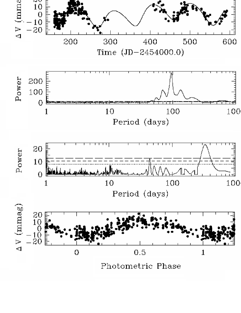
Figure 5: Top panel : Johnson V-band photometric observations of HIP 57050 from the 2006-07 and 2007-08 observing seasons acquired with a 0.35 m imaging telescope. The fitted line is the sum of a 98.1 days rotation period plus a second longer period component to track the seasonal drift. Second panel down : Power spectrum of the photometric data revealing strong periodicity, presumably due to spots on a star rotating at a period near 98 days. Third panel down : Power spectrum of the residuals from a best-fit photometric period of $98.1\pm 0.6$ days. The dominant peak near 333 days reflects season-to-season drifts in brightness due to long-term changes in the spot distribution. This drift is modeled here as the partial phase of a second sinusoidal component of period 328 days. Bottom panel : V-band observations from the top panel with season-to-season baseline drift removed, and phased with the 98.1 day photometric period. The peak-to-peak amplitude of the brightness variation is 0.023 mag.

Our goal with the photometric observations of HIP 57050 was to look for signs of activity and, if present, to find the star’s rotation period from the rotational modulation of features on the star’s photosphere (see, e.g., Henry et al., 1995). These observations help to determine if the radial velocity variations are caused by intrinsic stellar activity (Queloz et al., 2001) or by stellar reflex motion caused by the presence of an orbiting companion. We discarded the first 82 and the last 48 days of photometric measurements so that the remaining portion of the light curve exhibits reasonably coherent variability. We also discarded a few obvious outliers from the shortened light curve, which retains 314 measurements ranging over 433 days (see the top panel of Figure 5). Cyclic variability is easy to see. It is obvious from the top panel of Figure 5 that HIP 57050 is varying in brightness over a range of a couple percent on a timescale of approximately 100 days. A bootstrap analysis gives a rotation period of $98.1\pm 0.6$ days. The solid line corresponds to the sum of a 98.1 days rotation period and a second component with a longer period for removing the season-to-season drift. The missing portion of the light curve is due to the lack of observation between the two observing seasons.

The second panel of Figure 5 shows the power spectrum of the photometric data. As shown here, a strong periodicity exists near 98 days which is presumably due to spots on the star rotating at this rate. The third panel shows the spectrum of residuals from our best-fit photometric period of $98\pm 0.6$ days. The peak near 333 days is due to the season-to-season drifts in brightness which can be attributed to the long-term changes in the spot distribution. We have modeled this drift as the partial phase of a second sinusoidal component of period 328 days. The lesser peak near 45.5 days in the third panel is not significant and disappears when the 328 days component is fitted out, leaving no significant power at or near the 41.4 days Keplerian period in modeling either the full or shortened data sets.

The photometric observations are replotted in the bottom panel of Figure 5. Here the season-to-season baseline drift has been removed, and observations have been phased to the 98.1-day rotation period and a time of minimum computed from a least-squares sine fit. The sine fit also gives the peak-to-peak amplitude of 0.023 mag. The phase curve is slightly asymmetrical with the ascending branch shorter than the descending branch, as is often seen in the light curves of active stars (see Henry et al., 1995). That this period is clearly well separated from the radial velocity period argues strongly against stellar rotation as being the cause of the velocity variations and provides additional support for a planetary origin for the observed velocity variations.

6 Discussion

In the quest for potentially habitable planets, the nearest stars are of special importance. They have accurate distances and precisely determined stellar parameters, and are the only stars for which follow up by astrometry and direct imaging is possible. Within the Sun’s immediate neighborhood, M-dwarfs constitute the majority of nearby stars. As such, these stars have the special properties (distances, masses, and habitable zones) that drive exoplanetary science, astrobiology, and the next generation of interferometry and direct imaging missions. The habitable (liquid water) zones of nearby M-dwarfs are typically between 0.1 AU and 0.2 AU which corresponds to orbits with periods of 20 to 50 days. Establishing (by direct detection) the prevalence and nature of low-mass planets, such as HIP 57050 b, in these orbits informs us greatly about the possibility for potentially habitable planets (and/or moons) in the solar neighborhood.

A zeroth-order prediction of the core-accretion paradigm for giant planet formation is that the frequency of readily detectable giant planets should increase with both increasing stellar metallicity and with increasing stellar mass (Laughlin, Bodenheimer & Adams, 2004; Ida & Lin, 2005). During the past decade, both of these trends have been established observationally (see, e.g. Fischer & Valenti, 2005, for a discussion of the metallicity trend and Johnson et al. 2009 for a discussion of the mass trend). Until recently, however, there appeared to be little evidence for the strong expected planet-metallicity correlation among the handful of M-dwarf stars that are known to harbor giant planets. Attempts to determine accurate metallicities of M-dwarfs have largely been stymied by ambiguity in the continuum levels of their heavily line-blanketed spectra and by the profusion of molecular features in their spectra. Conventional estimates for the metallicities of 7 of the currently known planet-hosting M dwarfs as given by Bailey et al. (2009), and a comparison between these estimates and those of Schiavon et al. (1997) and Bean et al. (2006), suggest a spread of metallicity among these M-dwarfs (four are metal poor, one has high metallicity, and the metallicities of the remaining two are solar).

One would naively expect that a low-mass disk will need all the help it can get in order to build giant planet cores before the gas is gone. If anything, the planet-metallicity correlation should be strongest among the M-dwarfs. If observations show that the planet-metallicity correlation breaks down for M-dwarfs, then one is naturally led to speculate that the infrequent giant planets in a systems like Gliese 876 might be the outcome of gravitational instability (e.g. Boss, 2000) rather than core accretion.

Bonfils et al. (2005) pioneered a new approach to the determination of M-dwarf metallicities. The long evolutionary time scales for M-dwarfs imply that age-related $L$ and $T_{\rm eff}$ changes should be minimal once a low-mass star has landed on the zero-age main sequence. M-dwarf positions on the color-magnitude diagram, therefore, should be parameterized only by mass and metallicity, opening the possibility of a metallicity determination based on ${\rm M}_{\rm K}$ and V-K alone. Bonfils et al. (2005) developed such a calibration by assuming that M-dwarf binary companions to F, G, and K stars share the readily determined metallicities of their primaries. Johnson & Apps (2009) have recently provided an update to the Bonfils et al. (2005) calibration. The Johnson & Apps (2009) calibration indicates that the planet-bearing M-dwarfs do appear to be systematically metal-rich, suggesting that there is no breakdown of the planet-metallicity correlation as one progresses into the red dwarf regime.

HIP 57050 b appears to offer further support for the emerging M-dwarf planet-metallicity correlation. Using HIP 57050’s values, $V=11.88$, $K=6.822$, and $d=11.03\,{\rm pc}$, the Johnson & Apps (2009) calibration yields $[{\rm Fe/H}]=0.32\pm 0.06\,{\rm dex}$, indicating that HIP 57050 has a metallicity of order twice solar, which places it among the highest metallicity stars in the immediate solar neighborhood.

The a priori geometric transit probability for HIP 57050 b is $\sim 1\%$. The small size of the primary star and the planet’s unfavorable orbital alignment ($\omega=238^{\circ}$) conspire to diminish the odds that transits can be observed. An analysis of our photometry data also shows no signs of a transit. However, because the orbital elements can change if a second planet emerges, it is premature to conclude at this point that transits do not occur. The eclipse depth in this system is expected to be $\Delta F/F\sim 7\%$, which is considerably larger than that yet observed for any transiting planet. Such a large depth makes this system suitable for small-telescope observers to check. We therefore suggest that small-telescope observers carry out photometric monitoring of HIP 57050 during the predicted transit windows centered on HJD 2455201.400239. The large planet-to-star ratio would allow for detailed study of the atmosphere via transmission spectroscopy with HST. The expected planetary effective temperature, $T_{\rm eff}\sim 230\,{\rm K}$, suggests that the atmosphere may contain water clouds.

It is interesting to speculate about the possible presence of a habitable moon around HIP 57050 b. By analogy with our own solar system, whose gas giants all have dozens of moons, one might expect HIP 57050 b to also harbor such moons. In our solar system, $\sim 0.02\%$ of the masses of the gas giants are assigned to their satellites. This would translate to a satellite with $\sim 2\%$ of Earth’s mass (similar to Titan) orbiting HIP 57050 b. While it is not out of the question that HIP 57050 b could harbor a moon, and that moon would thus be in the liquid water habitable zone of the parent star, an object with only 1/5th of the mass of Mars in the liquid water habitable zone, from various standpoints is probably not a particularly good prospect for habitability. In any case, direct detection of such a moon would be extremely challenging.

We conclude this study by noting that the Doppler radial velocity method continues to be the most productive and cost-effective way to find those extrasolar planets that impart the greatest scientific returns (Butler et al., 2004; Rivera et al., 2005; Lovis et al., 2006; Udry et al., 2007; Mayor & Udry, 2008; Vogt et al., 2010; Rivera et al., 2010). During the past several years, the threshold $M\sin(i)$ for radial velocity planets has rapidly approached the 1$M_{\oplus}$ regime. Radial velocity surveys, furthermore, have led to the discovery of all but one of the most readily characterizable transiting planets, and the rapidly growing catalog of Doppler-detected planets has been instrumental in providing our best current view of the nearby planetary population. The future looks bright!

Figure 1: Relative radial velocities for HIP 57050 obtained with the HIRES spectrometer on the Keck I telescope. The zero point is arbitrary and set to the mean of all the velocities.

Figure 2: Top panel - Keplerian periodogram of the radial velocity data set for HIP 57050. The power plotted at each sampled period is proportional to the relative improvement (drop in $\chi_{\nu}^{2}$) in the fit quality for the best Keplerian found at that period versus a constant velocity model. The horizontal lines in this and all similar figures indicate (top to bottom) False Alarm Probability (FAP) levels of 0.1%, 1%, and 10.0% respectively. The dominant peak in the top panel corresponds to the best-fit Keplerian orbit. Bottom panel - Power spectral window (periodogram of the times of observation).

Figure 3: Best one-planet Keplerian fit to the phased Keck-HIRES relative radial velocities of HIP 57050.

Figure 4: Top: Circular periodogram of residuals from a 1-planet fit. Bottom: Circular periodogram of residuals from a 1-planet fit+trend fit.

Table 1: Stellar Parameters for HIP 57050

Parameter	Value	Reference
Spectral Type	M4	Reid et al. (2004)
Mass ($M_{\odot}$)	0.34$\pm$0.03	This work
Radius ($R_{\odot}$)	0.4	This work
Luminosity ($L_{\odot}$)	0.01486	This work
Distance (pc)	11.0$\pm$0.4	Perryman et al. (1997)
$B-V$	1.60	(Perryman et al., 1997; Kharchenko, 2001)
$V$ Mag.	11.881$\pm$0.004	(Perryman et al., 1997; Kharchenko, 2001)
$J$ Mag.	7.608	(Cutri et al., 2003)
$H$ Mag.	7.069	(Cutri et al., 2003)
$K$ Mag.	6.822	(Cutri et al., 2003)
$\log{R^{\prime}_{\rm HK}}$	-5.31	This work
$P_{\rm rot}$ (days)	98	This work
$T_{\rm eff}$ (K)	3190	Morales et al. (2008)
$M_{{\rm bol},\,\odot}$	9.32	Morales et al. (2008)
$\log{g}$	4.67	This work

Table 2: Relative Radial Velocities for HIP 57050

JD (-2450000)	RV (m s-1)	Uncertainty (m s-1)
1581.04559	-62.47	2.83
1705.82690	-60.65	3.12
1983.00875	-8.54	3.66
2064.86395	0.55	3.63
2308.07715	7.74	2.92
2391.03363	1.16	4.27
2681.05010	-1.92	3.41
2804.88465	12.67	3.42
3077.10434	-32.24	3.99
3398.97476	-20.67	2.78
3753.06771	7.44	3.18
4131.09206	13.39	3.47
4545.00223	0.62	2.84
4546.00720	0.00	2.62
4600.90598	-32.56	2.76
4671.81115	-13.12	3.66
4686.77023	-53.48	3.49
4819.09864	5.22	2.10
4820.10874	15.76	2.21
4821.17169	18.42	3.48
4822.16958	16.55	2.91
4823.07178	32.62	1.91
4903.13549	12.10	3.26
4967.95619	-31.62	2.80
4968.94631	-33.00	2.12
5021.75704	-24.72	2.54
5022.80694	-9.14	2.18
5024.80704	3.99	1.96
5049.74445	-24.81	2.05
5050.74198	-15.34	2.16
5051.74421	-24.64	2.44
5052.74328	-9.64	2.52
5053.74585	-29.42	2.12
5168.06193	16.20	2.37
5201.00003	30.44	2.61
5202.07289	30.08	2.12
5203.11589	26.33	2.02

Table 3: Keplerian Fit to the RV Data for HIP 57050

Parameter	Value (one-planet fit)	Value (one-planet fit+trend)
$P$ (days)	$41.397\pm 0.016$	$41.352\pm 0.050$
$m\sin{i}$ ($M_{\rm J}$)	$0.298\pm 0.025$	$0.276\pm 0.021$
$a$ (AU)	$0.163506\pm 0.000042$	$0.16338\pm 0.00013$
$K$ (m s-1)	$37.8\pm 4.5$	$34.0\pm 2.8$
$e$	$0.314\pm 0.086$	$0.194\pm 0.073$
$\omega$ (deg.)	$238.1\pm 23.2$	$258.3\pm 36.8$
MA (deg.)	$321.1\pm 21.2$	$273.1\pm 55.4$
$\chi_{\nu}^{2}$	13.50	10.14
RMS (m s-1)	9.23	8.06
trend (m s${}^{-1}\,d^{-1}$)	-	$0.00675\pm 0.0033$

References

- Bailey et al. (2009) Bailey, J., Butler, R. P., Tinney, C. G., Hugh, R. A. J., O’Toole, S., Carter, B. D., & Marcy, G. W. 2009, ApJ, 690, 743
- Bean et al. (2006) Bean, J. L., Benedict, G. F., & Endl, M. 2006, ApJ, 653, L65
- Bonfils et al. (2005) Bonfils, X., Delfosse, X., Udry, S., Santos, N. C., Forveille, T., & Ségransan, D. 2005, A&A, 442, 635
- Boss (2000) Boss, A. P. 2000, ApJ, 536, L101
- Boss (2006) Boss, A. P. 2006, ApJ, 644, L79
- Butler et al. (1996) Butler, R. P., Marcy, G. W., Williams, E., McCarthy, C., Dosanjh, P., & Vogt, S. S. 1996, PASP, 108, 500
- Butler et al. (2004) Butler, R. P., Vogt, S. S., Marcy, G. W., Fischer, D. A., Wright, J. T., Henry, G. W., Laughlin, G., & Lissauer, J. J. 2004, ApJ, 617, 580
- Cumming (2004) Cumming, A. 2004, MNRAS, 354, 1165
- Cutri et al. (2003) Cutri, R. M., et al. 2003, 2MASS All Sky Catalog of point sources
- Deeming (1975) Deeming, T. J. 1975, AP&SS, 36, 137
- Fischer & Valenti (2005) Fischer, D. A., & Valenti, J. 2005, ApJ, 662, 1102
- Forget & Pierrehumbert (1997) Forget, F., & Pierrerhumbert, R. T. 1997, Science, 278, 1273
- Gilliland & Baliunas (1987) Gilliland, R. L., & Baliunas, S. L. 1987, ApJ, 314, 766
- Grenfell et al. (2007) Grenfell et al. 2007, Astrobiology, 7, 208
- Henry & McCarthy (1993) Henry, T. J., & McCarthy, D. W. 1993, AJ, 106, 773
- Henry et al. (1995) Henry, G. W., Fekel, F. C., & Hall, D. S. 1995, AJ, 110, 2926
- Ida & Lin (2005) Ida, S., & Lin, D. N. C. 2005, ApJ, 626, 1045
- Johnson & Apps (2009) Johnson, J. A., & Apps, K. 2009, ApJ, 699, 933
- Johnson et al. (2009) Johnson et al. 2009, PASP, 122, 149
- Jones et al. (2006) Jones, B. W., Sleep, P. N., & Underwood, D. R., 2006, ApJ, 649, 1010
- Joshi et al. (1997) Joshi, M. M., Haberle, R. M., Reynolds, R. T. 1997, Icarus, 129, 450
- Kasting et al. (1993) Kasting, J. F., Whitmire, D. P., & Reynolds, R. T. 1993, Icarus, 101, 108
- Kharchenko (2001) Kharchenko, N. V. 2001, Kinematika Fiz. Nebesn. Tel., 17, 409
- Laughlin, Bodenheimer & Adams (2004) Laughlin, G., Bodenheimer, P., & Adams, F. C. 2004, ApJ, 612, L73
- Lovis et al. (2006) Lovis, C., et al. 2006, Nature, 441, 305
- Mayor & Udry (2008) Mayor, M., & Udry, S. 2008, Physica Scripta, 130, 014010
- Meschiari et al. (2009) Meschiari, S., Wolf, A. S., Rivera, E. J., Laughlin, G., Vogt, S. S., & Butler, R. P. 2009, PASP, 121, 1016
- Mischna et al. (2000) Mischna, M. A., Kasting, J. F., Pavlov, A., & Freedman, R. 2000, Icarus, 145, 546
- Morales et al. (2008) Morales, J. C., Ribas, I., & Jordi, C. 2008, A&A, 478, 507
- Perryman et al. (1997) Perryman, M. A. C., et al. 1997, A&A, 323, L49. The Hipparcos Catalog
- Queloz et al. (2001) Queloz et al. 2001, A&A, 379, 279
- Reid et al. (2004) Reid et al. 2004, AJ, 128, 463
- Rivera et al. (2005) Rivera et al. 2005, ApJ, 634, 625
- Rivera et al. (2010) Rivera, E. J., Butler, R. P., Vogt, S. S., Laughlin, G., Henry, G. W., & Meschiari, S. 2010, ApJ, 708, 1492
- Scalo et al. (2007) Scalo et al. 2007, Astrobiology, 7, 85
- Schiavon et al. (1997) Schiavon, R. P., Barbuy, B., & Singh, P. D. 1997, ApJ, 484, 499
- Segura et al. (2005) Segura, A., Kasting, J. F., Meadows, V., Cohen, M., Scalo, J., Crisp, D., Butler, R. A. H., & Tinetti, G. 2005, Astrobiology, 5, 706
- Selsis et al. (2007) Selsis, F., Kasting, J. F., Levrard, B., Paillet, J., Ribas, I., & Delfosse, X. 2007, A&A, 476, 1373
- Tarter et al. (2007) Tarter, J. C., et al. 2007, Astrobiology, 7., 30
- Udry et al. (2007) Udry, S., et al. 2007, A&A, 469, L43
- Vogt et al. (1994) Vogt, S. S., et al. 1994, SPIE, 2198, 362
- Vogt et al. (2010) Vogt, S. S., et al. 2010, ApJ, 708, 1366
- Williams & Pollard (2002) Williams, D. M., & Pollard, D., 2002, Int. J. Astrobiol., 1, 61