Smoothed Particle Hydrodynamics simulations of white dwarf collisions and close encounters

Abstract

The collision of two white dwarfs is a quite frequent event in dense stellar systems, like globular clusters and galactic nuclei. In this paper we present the results of a set of simulations of the close encounters and collisions of two white dwarfs. We use an up-to-date smoothed particle hydrodynamics code that incorporates very detailed input physics and an improved treatment of the artificial viscosity. Our simulations have been done using a large number of particles ($\sim 4\times 10^{5}$) and covering a wide range of velocities and initial distances of the colliding white dwarfs. We discuss in detail when the initial eccentric binary white dwarf survives the closest approach, when a lateral collision in which several mass transfer episodes occur is the outcome of the newly formed binary system, and which range of input parameters leads to a direct collision, in which only one mass transfer episode occurs. We also discuss the characteristics of the final configuration and we assess the possible observational signatures of the merger, such as the associated gravitational waveforms and the fallback luminosities. We find that the overall evolution of the system and the main characteristics of the final object agree with those found in previous studies. We also find that the fallback luminosities are close to $10^{48}$ erg/s. Finally, we find as well that in the case of lateral and direct collisions the gravitational waveforms are characterized by large-amplitude peaks which are followed by a ring-down phase, while in the case in which the binary white dwarf survives the closest approach, the gravitational pattern shows a distinctive behavior, typical of eccentric systems.

1 Introduction

In recent years, the study of stellar collisions has attracted much interest from the astronomical community working on the dynamics of dense stellar systems, like the cores of globular clusters and galactic nuclei (Shara 2002). One of the reasons for this is that in these systems, stellar collisions are rather frequent (Hills & Day 1976). In fact, it has been predicted that up to 10% of the stars in the core of typical globular clusters have undergone a collision at some point during the lifetime of the cluster (Davies 2002).

The most probable collisions are those in which at least one of the colliding stars has the largest possible cross section — a red giant — and those in which at least one of the stars is most common (Shara & Regev 1986). This later type of collisions obviously includes those in which a main sequence star is involved. However, because white dwarfs are the most common end point of stellar evolution and because both globular clusters and galactic nuclei are rather old, these stellar systems contain many collapsed and degenerate objects. Therefore, we expect that collisions in which one of the colliding stars is a white dwarf should be rather common.

Collisions between two main sequence stars are supposed to be responsible for the observed population of blue stragglers in globular clusters (Sills & Bailyn 1999; Sills et al. 2005). Although the collision between a main sequence star and a red giant is more probable than that of two main sequence stars because of the larger geometrical cross section of the red giant star, they probably do not produce an interesting astrophysical object. The reason for this is the low density of the envelopes of red giants. In most cases, during the encounter the red giant is deprived of part of its envelope and is able to recover its appearance (Freitag & Benz 2005). The collisions of a white dwarf and a red giant or a main sequence star are also of large interest, since they may be responsible for the formation of some interesting astrophysical objects. Unfortunately, due to the very different dynamical scales involved, the hydrodynamical simulation of these events is difficult and realistic simulations of their outcome are still lacking. However, in the case in which a red giant and a white dwarf collide it is thought that the most probable outcome is the ejection of the envelope of the red giant and the formation of a double white dwarf binary system (Tuchman 1985), whilst in the case in which a main sequence star and a white dwarf collide it has been shown (Shara & Regev 1986) that only a small fraction of the disrupted main sequence star remains bound to the white dwarf. More recent simulations (Ruffert 1992) predict the formation of a disk around the white dwarf. However, we emphasize that all these simulations used rudimentary input physics and, thus, the outcomes of these simulations are dubious.

The collision of two white dwarfs deserves study for various reasons. In particular, the collision of two white dwarfs can produce a Type Ia supernova. Although the most standard scenario for a Type Ia outburst — the so-called single-degenerate scenario — involves a white dwarf accreting from a non-degenerate companion, the double-degenerate scenario (Webbink 1984; Iben & Tutukov 1984), in which the merging of two carbon-oxygen white dwarfs with a total mass larger than the Chandrasekhar limit occurs, has been one of the most favored scenarios leading to Type Ia supernovae. In fact, it has been predicted that the white dwarf merger rate leading to super-Chandrasekhar remnants will be increased by an order of magnitude through dynamical interactions (Shara & Hurley 2002). Therefore, collisions of two white dwarfs of sufficiently large masses could explain supernovae occurring in the nuclei of galaxies. Moreover, it has been recently suggested that such a process would lead to both a Type Ia supernova explosion and to the formation of a magnetar (King, Pringle & Wickramasinghe 2001). This scenario would explain the main characteristics of soft gamma-ray repeaters and anomalous X-ray pulsars like 1E2259+586. Also, dynamical interactions in globular clusters can form double white dwarfs with non-zero eccentricities, which would be powerful sources of gravitational radiation (Willems et al. 2007). Moreover, the initial stages of the coalescence of a white dwarf binary system could be one of the most interesting sources for the detection of gravitational waves using space-borne detectors like LISA (http://lisa.jpl.nasa.gov). Thus, a close encounter of two white dwarfs would be a potentially observable source of gravitational waves and, hence, characterizing the gravitational waveforms is also of interest. Finally, the temperatures achieved in a direct collision are substantially high and, consequently, we expect that some of the nuclearly processed material could be ejected, leading to a pollution of the environment where it occurs, either a globular cluster or a galactic nucleus.

Despite of its potential interest, there are very few simulations of the collision of two white dwarfs, the only exception being those of Benz et al. (1989), Rosswog et al. (2009) and Raskin et al. (2009). All three sets of simulations used Smoothed Particle Hydrodynamics (SPH) to model the collisions. However, the simulations of Benz et al. (1989) were done using a small number of particles whereas those of Rosswog et al. (2009) and Raskin et al. (2009) have studied a limited range of impact parameters. To be specific, the simulations of Benz et al. (1989) used $5\times 10^{3}$ particles, while those of Rosswog et al. (2009) and Raskin et al. (2009) used, respectively, $2.5\times 10^{6}$ and $8\times 10^{5}$ SPH particles. The very recent simulations of Rosswog et al. (2009) and Raskin et al. (2009) were aimed to produce a thermonuclear explosion and, thus, they only studied direct collisions, while the simulations of Benz et al. (1989) covered a broader range of initial conditions. Additionally, in the early work of Benz et al. (1989) the classical expression for the artificial viscosity (Monaghan & Gingold 1983) was used, while in the very recent calculations of Rosswog et al. (2009) and Raskin et al. (2009) more elaborated prescriptions for the artificial viscosity were employed.

In sharp contrast, the coalescence of binary white dwarfs was extensively studied in the past and also has been the object of several recent studies. For instance, the pioneering works of Mochkovitch & Livio (1989, 1990) used an approximate method — the so-called Self-Consistent-Field method (Clement 1974) — while the full SPH simulations of Benz, Thielemann & Hills (1989), Benz, Cameron & Bowers (1989), Benz, Hills & Thielemann (1989), Benz et al. (1990), Rasio & Shapiro (1995) and Segretain, Chabrier & Mochkovitch (1997) studied the problem using reduced resolutions and the classical expression for the artificial viscosity (Monaghan & Gingold 1983). Later, Guerrero et al. (2004) opened the way to more realistic simulations, using an increased number of SPH particles and an improved prescription for the artificial viscosity. More recently, the simulations of Yoon et al. (2007) and of Lorén–Aguilar et al. (2005, 2009) were carried out using modern prescriptions for the artificial viscosity and even larger numbers of particles. All in all, it is noticeable the lack of SPH simulations of white dwarf collisions and close encounters when compared to the available literature on white dwarf mergers.

In the present paper we study the collision of two white dwarfs employing an enhanced spatial resolution ($4\times 10^{5}$ SPH particles) and an improved formulation for the artificial viscosity. We pay special attention to discern the range of initial conditions that produce the tidal disruption of the less massive white dwarf or those for which the initial eccentric binary survives the closest approach. The number of particles used in our simulations is much larger than those used in the simulations of Benz et al. (1989) and in line with those used in modern simulations (Rosswog et al. 2009; Raskin et al. 2009). However, our calculations encompass a broad range of initial conditions of the colliding white dwarfs, in contrast to most modern simulations, in which only a few cases were studied in detail. The paper is organized as follows. In §2 we describe our input physics and the method of calculation, paying special attention to describe with some detail our SPH code. It follows §3, which is devoted to discuss the initial conditions adopted in the present study, while in §4 we describe the results of our simulations. Finally in §4 we summarize our main findings and draw our conclusions.

2 Input physics and method of calculation

We follow the hydrodynamic evolution of the interacting white dwarfs using a Lagrangian particle numerical code, the so-called Smoothed Particle Hydrodynamics. This method was first proposed by Lucy (1977) and, independently, by Gingold & Monaghan (1977). The fact that the method is totally Lagrangian and does not require a grid makes it especially suitable for studying an intrinsically three-dimensional problem like the collision of two white dwarfs. We will not describe in detail the most basic equations of our numerical code, since this is a well-known technique. Instead, the reader is referred to Benz (1990) where the basic numerical scheme for solving the hydrodynamic equations can be found, whereas a general introduction to the SPH method can be found in the excellent review of Monaghan (2005). However, and for the sake of completeness, we briefly describe the most relevant equations of our numerical code.

We use the standard polynomic kernel of Monaghan & Lattanzio (1985). The gravitational forces are evaluated using an octree (Barnes & Hut 1986). Also, gravitational forces between SPH particles are softened using the procedures described in Monaghan & Gingold (1977) and Hernquist & Katz (1989). Our SPH code uses a prescription for the artificial viscosity based in Riemann-solvers (Monaghan 1997). Additionally, to suppress artificial viscosity forces in pure shear flows, we also use the viscosity switch of Balsara (1995). In this way the dissipative terms are largely reduced in most parts of the fluid and are only used where they are really necessary to resolve a shock, if present. Within this approach, the SPH equations for the momentum and energy conservation read, respectively, as

$$\frac{d\vec{v}_{i}}{dt}= - \sum_{j}m_{j}\left(\frac{P_{i}}{\rho_{i}^{2}}+\frac{P_{j}}{\rho_{j}^{2}}-\alpha\overline{f}_{ij}\frac{v^{\rm sig}_{ij}}{\overline{\rho}_{ij}}\vec{v}_{ij}\cdot\hat{e}_{ij}\right)$$ (1)

$$\vec{r}_{ij}\overline{F}_{ij}$$

$$\frac{du_{i}}{dt}= \frac{P_{i}}{\rho_{i}^{2}}\sum_{j}m_{j}\vec{v}_{ij}\cdot\vec{r}_{ij}\overline{F}_{ij}$$ (2)

$$- \frac{1}{2}\sum_{j}m_{j}\alpha\overline{f}_{ij}\frac{v^{\rm sig}_{ij}}{\overline{\rho}_{ij}}(\vec{v}_{ij}\cdot\hat{e}_{ij})^{2}|\vec{r}_{ij}|\overline{F}_{ij}$$

where $\overline{f}_{ij}=(f_{i}+f_{j})/2$ and

$$f_{i}=\frac{|\nabla\cdot\vec{v}|_{i}}{|\nabla\cdot\vec{v}|_{i}+|\nabla\times\vec{v}|_{i}+10^{-4}{c_{i}}/{h_{i}}},$$ (3)

In these expressions $\vec{r}_{ij}=\vec{r}_{i}-\vec{r}_{j}$, $\vec{v}_{ij}=\vec{v}_{i}-\vec{v}_{j}$, $\hat{e}_{ij}=\vec{r}_{ij}/|\vec{r}_{ij}|$, $\overline{\rho}_{ij}=(\rho_{i}+\rho_{j})/2$, $\overline{F_{ij}}=(F_{i}+F_{j})/2$, and $F$ is a function that only depends on $|\vec{r}|$ and on the smoothing kernel $h_{i}$ used to express the gradient of the kernel $\vec{\nabla}W_{ij}=\overline{F}_{ij}\vec{r}_{ij}$. The rest of the symbols have their usual meaning. The signal velocity is taken as $v^{\rm sig}_{ij}=c_{i}+c_{j}-4\vec{v}_{ij}\cdot\hat{e}_{ij}$, where $c_{i}$ is the sound speed of particle $i$. Note that in the expression for the signal velocity we have arbitrarily fixed the coefficient of the relative velocity, $\vec{v}_{ij}$, to the value recommended by Monaghan (2005). We find that $\alpha=0.5$ yields good results.

We have found that it is sometimes advisable to use a different formulation of the equation of energy conservation. Accordingly, for each time step we compute the variation of the internal energy using Eq. (2) and simultaneously calculate the variation of the temperature using

$$\frac{dT_{i}}{dt}= - \sum_{j}\frac{m_{j}}{(C_{v})_{j}}\frac{T_{j}}{\rho_{i}\rho_{j}}\left[\left(\frac{\partial P}{\partial T}\right)_{\rho}\right]_{j}\vec{v}_{ij}\cdot\vec{r}_{ij}\overline{F}_{ij}$$ (4)

$$- \frac{1}{2}\sum_{j}\frac{m_{j}}{(C_{v})_{j}}\alpha\overline{f}_{ij}\frac{v^{\rm sig}_{ij}}{\overline{\rho}_{ij}}(\vec{v}_{ij}\cdot\hat{e}_{ij})^{2}|\vec{r}_{ij}|\overline{F}_{ij}$$

where $C_{v}=(\partial U/\partial T)_{V}$ is the specific heat capacity per unit mass — see Timmes & Arnett (1999) and Segretain et al. (1994) and references therein for more details about the implementation of the equation of state. For regions in which the temperatures are lower than $6\times 10^{8}$ K or the densities are lower than $6\times 10^{3}$ g/cm³, Eq. (2) is adopted, whereas Eq. (4) is used in the rest of the fluid. We adopt this procedure because the internal energy of degenerate electrons depends very weakly on the temperature. Thus, in the region where degeneracy is large small variations of the internal energy can produce large fluctuations of the temperature. The use of Eq. (4) avoids numerical artifacts and allows to use longer time steps. Using this prescription we find that energy is best conserved. Specifically, we find that, depending on the run, energy is conserved to accuracies ranging from 0.1% to 3.2%. Angular momentum is conserved to an accuracy of 0.1% in the worst of the cases.

Run	$y_{\rm ini}$	$v_{\rm ini}$	Outcome	$E$	$L$	$r_{\max}$	$r_{\min}$	$\varepsilon$	$\beta$
	($R_{\sun}$)	(km/s)		($10^{48}$ erg)	($10^{50}$ erg/s)	(0.1 $R_{\sun}$)	(0.1 $R_{\sun}$)
1	0.8	100	O	$-2.13$	7.49	8.28	0.50	0.886	0.40
2	0.5	150	O	$-3.17$	7.02	5.46	0.45	0.848	0.44
3	0.5	50	DC	$-3.44$	2.33	5.39	0.05	0.983	4.00
4	0.3	225	O	$-4.49$	6.31	3.80	0.37	0.823	0.54
5	0.3	200	LC	$-4.64$	5.62	3.75	0.29	0.858	0.69
6	0.3	175	LC	$-4.77$	4.91	3.71	0.21	0.891	0.95
7	0.3	150	LC	$-4.88$	4.21	3.68	0.16	0.919	1.25
8	0.3	125	LC	$-4.98$	3.51	3.66	0.11	0.943	1.82
9	0.3	100	DC	$-5.05$	2.81	3.64	0.07	0.964	2.86
10	0.1	200	DC	$-7.82$	1.87	2.36	0.03	0.975	6.67
11	0.1	150	DC	$-8.06$	1.40	2.31	0.02	0.986	10.0
12	0.1	120	DC	$-8.16$	1.17	2.28	0.01	0.990	20.0

Table 1: Summary of the kinematical properties of the $0.6+0.8\,M_{\sun}$ simulations. Note that the radius of the less massive white dwarf is $R_{2}\sim 0.01\,R_{\sun}$. Energy and angular momentum have been calculated in the center of mass frame. The results presented here correspond to the SPH calculations.

The algorithm used to determine the smoothing length of each particle is that of Hernquist & Katz (1989). That is, we determine the new smoothing length taking into account the previous one and imposing that the new one should be such that the average number of neighbour particles should remain constant. In our calculations we adopt 32 neighbour particles. For the integration method, we use a predictor-corrector numerical scheme with variable time steps (Serna, Alimi & Chieze 1996), which turns out to be quite accurate. Each particle is followed with individual time steps. Time steps are determined comparing the local sound velocity with the local acceleration and imposing that none of the SPH particles travels a distance larger than its corresponding smoothing length. We also impose that the temperature or the energy do not vary in one time step by more than 5%.

The equation of state adopted for the white dwarf is the sum of three components. The ions are treated as an ideal gas but we take the Coulomb corrections into account (Segretain et al. 1994). We have also incorporated the pressure of photons, which turns out to be important when the temperature is high and the density is small, just when nuclear reactions become relevant. Finally the most important contribution is the pressure of degenerate electrons, which is treated by integrating the Fermi-Dirac integrals. The nuclear network adopted here incorporates 14 nuclei: He, C, O, Ne, Mg, Si, S, Ar, Ca, Ti, Cr, Fe, Ni, and Zn. The reactions considered are captures of $\alpha$ particles, and the associated back reactions, the fussion of two C nuclei, and the reaction between C and O nuclei. All the rates are taken from Rauscher & Thielemann (2000). The screening factors adopted in this work are those of Itoh et al. (1979). The nuclear energy release is computed independently of the dynamical evolution with much shorter time steps, assuming that the dynamical variables do not change much during these time steps. Finally, neutrino losses have also been included according to the formulation of Itoh et al. (1996) for the pair, photo, plasma, and bremsstrahlung neutrino processes.

In order to explore a wide range of input parameters we have relaxed two initial carbon-oxygen white dwarf models with masses $M_{1}=0.8\,M_{\sun}$ and $M_{2}=0.6\,M_{\sun}$, respectively. Carbon and oxygen in these models have equal mass abundances and are uniformly distributed. The temperature of our isothermal white dwarf initial models is $T=10^{7}$ K, a rather typical value. To achieve equilibrium initial configurations, each individual model star was relaxed separately, so the two interacting white dwarfs are spherically symmetric at the beginning of our simulations, as was the case in all previous simulations of this kind. Finally, we emphasize that to avoid numerical artifacts, we only use equal-mass SPH particles. Consequently, the $0.8\,M_{\sun}$ white dwarf was relaxed using $\sim 2.6\times 10^{5}$ SPH particles, whereas the $0.6\,M_{\sun}$ white dwarf needed $\sim 2.0\times 10^{5}$ SPH particles. However, we would like to note that we also performed some additional runs in which the number of particles was a factor of 10 smaller, and we obtained essentially the same results. Neverteless, these simulations are not presented here. The central densities of the white dwarfs are, respectively, $\rho_{1}\simeq 1.0\times 10^{7}$ g/cm³ and $\rho_{2}\simeq 3.6\times 10^{6}$ g/cm³, while their respective moments of inertia (which are important for discussing of our results) are $I_{1}\simeq 2.50\times 10^{50}$ g cm² and $I_{2}\simeq 2.68\times 10^{50}$ g cm². Finally the radii of the isolated white dwarfs are, respectively, $R_{1}\simeq 0.009\,R_{\sun}$ and $R_{2}\simeq 0.011\,R_{\sun}$.

3 Initial conditions

We have fixed the initial distance between the stars along the $x$ axis, $x_{\rm ini}$, and their angular velocity, $\omega$, allowing the initial distance along the $y$ axis, $y_{\rm ini}$, and the initial velocity of each of the stars $\vec{v}_{i}=(\pm v_{\rm ini},0,0)$ to be our free parameters. Note that the relative velocity of the intervening white dwarfs is thus $2v_{\rm ini}$. The initial distance at which the two interacting white dwarfs are placed is always $x_{\rm ini}=0.2\,R_{\sun}$, which is much larger than the radii of the intervening white dwarfs ($\sim 0.01\,R_{\sun}$). Under these conditions the tidal deformations of both white dwarfs are negligible at the beginning of the simulation and the approximation of spherical symmetry is valid. Note that with this setting the initial coordinates of both stars are $(+x_{\rm ini}/2,-y_{\rm ini}/2,0)$ and $(-x_{\rm ini}/2,+y_{\rm ini}/2,0)$, and the center of mass moves with a total velocity $v_{\rm cm}=v_{\rm ini}/7$ in the $xy$ plane. The two interacting white dwarfs have rotational velocities $\omega\simeq 7\times 10^{-5}$ rad/s and are assumed to rotate counterclockwise. These velocities are representative of those found in field white dwarfs (Berger et al. 2005). We have also assumed that the white dwarfs rotate as rigid solids (Charpinet et al. 2009).

We have conducted 12 simulations with initial distances ranging from $0.1\,R_{\sun}$ to $0.8\,R_{\sun}$ and initial velocities from 50 to 225 km/s — see Table 1 for a summary of the initial conditions adopted for each of the simulations presented here. It has to be noted that we have restricted our attention to the post-capture scenario. Consequently, all the systems studied here were bound from the start. For a detailed study of the gravitational capture mechanisms see, for example, Press & Teukolsky (1977) and Lee & Ostriker (1986). We note, however, that in order for a pair of stars to become bound after a close encounter, some kind of dissipation mechanism must be involved. Some examples of dissipation mechanisms are a third body tidal interaction (Shara & Hurley 2002) or the excitation of stellar pulsations by means of tidal interaction (Fabian et al. 1975).

The typical stellar dispersion velocity in globular clusters $v_{\rm d}$ is approximately 10 km/s while the relative velocity $v_{\rm c}$ in a close encounter — assuming an interaction distance $r_{\min}\lesssim 1R_{\sun}$ — for a pair of stars can be shown to be (Fabian et al. 1975)

$$v_{\rm c}\simeq\left(2G\frac{M_{1}+M_{2}}{r_{\min}}\right)^{1/2}\gtrsim 100~{}{\rm km/s}$$ (5)

where $M_{1}$ and $M_{2}$ are the masses of the interacting stars and $r_{\min}$ is the distance at periastron. Thus, only $\sim\left(v_{\rm d}/v_{\rm c}\right)^{2}\lesssim 0.01$ of the kinetic energy available at closest approach needs to be dissipated in order to bound the system. This fraction is small enough to expect a relatively high formation rate of this type of systems (Lee & Ostriker 1986). However, given our initial conditions, which result in eccentricities $\varepsilon\sim 0.9$ (a typical value in the simulations presented here, see table 1) more energy dissipation than it is reasonable to expect from a single periastron passage is needed. Hence, at least some of the collisions presented here are more likely to result from encounters involving three or more stars than they are from a traditional tidal capture (Ivanova et al. 2006).

4 Results

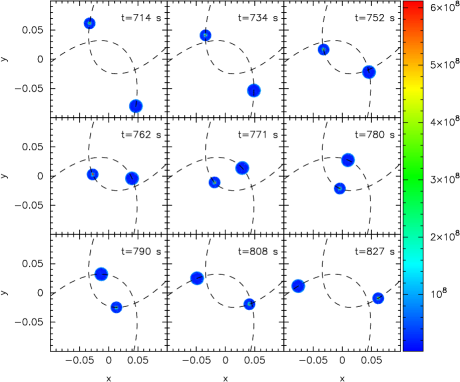
Figure 1: Time evolution of one of the simulations in which the eccentric double white dwarf system survives closest approach. In particular, this simulation corresponds to the case in which the initial velocity is $v_{\rm ini}=150$ km/s and the initial distance is $y_{\rm ini}=0.5R_{\sun}$. The temperatures of each SPH particle are also shown, expressed in K, while the $x$ and $y$ axes are in units of solar radius. The dashed lines correspond to the trajectories of the center of mass of each star. Only 1 out of 10 particles has been represented. Times are shown in the right upper corner of each panel. These figures have been done using the visualization tool SPLASH (Price 2007). [Color figure only available in the electronic version of the article].

Depending on the kinetic energy dissipated during the encounter two different outcomes might result: if the stars get sufficiently close at periastron and mass transfer begins, a stellar merger will occur, otherwise the eccentric binary system will survive the closest approach. We have obtained three distinct behaviors, depending on the input parameters of the close encounter: direct collisions, lateral collisions — characterized by more than one mass-transfer episode previous to the stellar merger — and, finally, eccentric binary systems surviving the closest approach. Three representative examples of each of these cases are shown, respectively, in figures 1, 2 and 3.

4.1 Dynamics and outcomes of the interactions

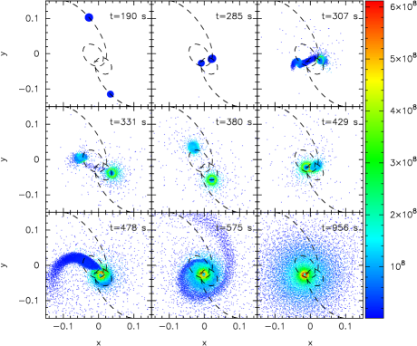
Figure 2: Same as figure 1 for one of the simulations in which the outcome is a lateral collision. In particular, this corresponds to the case in which $v_{\rm ini}=175$ km/s and $y_{\rm ini}=0.3R_{\sun}$. [Color figure only available in the electronic version of the article].

In figure 1 we show the time evolution of one of the cases in which the eccentric binary survives the closest approach. In particular, this figure corresponds to the case in which a pair of white dwarfs of masses $0.6$ and $0.8~{}M_{\sun}$ interacts with initial parameters $v_{\rm ini}=150$ km/s and $y_{\rm ini}=0.5~{}R_{\sun}$. The dashed line depicts the motion of the center of masses of each white dwarf. As can be seen, the orbits are elliptical and the temperatures of the intervening white dwarfs remain constant. In figure 2 we show an example of a lateral collision, corresponding to the same intervening white dwarfs, but now the initial conditions are $v_{\rm ini}=175$ km/s and $y_{\rm ini}=0.3~{}R_{\sun}$. In this case the two interacting white dwarfs perform a first passage through the periastron during which a first mass-transfer episode occurs — see the top three panels of figure 2. After this mass-transfer episode the two white dwarfs become detached — left and middle central panels of figure 2. Subsequently, the two white dwarfs approach again each other and a second mass-transfer episode ensues — right central panel of figure 2. This second mass-transfer episode is unstable and the white dwarfs coalesce. The less massive white dwarf forms an spiral arm — left bottom panel — which, as a consequence of the orbital motion, entangles — middle bottom panel — and, finally, forms a heavy keplerian disk — right bottom panel — very much in the same manner as it occurs in the case of coalescing binaries (Lorén–Aguilar et al. 2009). Finally, in figure 3 we display an example of a direct collision, corresponding to the case in which two white dwarfs of masses $0.6$ and $0.8~{}M_{\sun}$ with initial parameters $v_{\rm ini}=120$ km/s and $y_{\rm ini}=0.1~{}R_{\sun}$ collide. As can be seen in this figure, during the first stages of the encounter both white dwarfs preserve their original spherical shape and their temperatures remain stable — top panels of figure 3. At $t\simeq 134$ s — left central panel — the two white dwarfs collide and the material increases considerably the temperature, reaching temperatures as high as $T\sim 9\times 10^{8}$. As a result of the direct collision, the SPH particles acquire very large velocities — right central panel of figure 3 — and the cloud of SPH particles expands. Initially, the expansion of this cloud of particles is not perfectly symmetric — left bottom panel of figure 3 — but at time passes by, a spherically symmetric cloud forms — right bottom panel of figure 3.

Run	$M_{\rm WD}$	$M_{\rm debris}$	$M_{\rm ej}$	$T_{\max}$	$T_{\rm peak}$	$R_{\rm debris}$	$\Delta t$	$E_{\rm nuc}$	$E_{\nu}$	$E_{\rm GW}$
3	1.00	0.40	$1.6\times 10^{-2}$	$5.9\times 10^{8}$	$1.6\times 10^{9}$	0.2	150	$2.5\times 10^{44}$	$3.6\times 10^{30}$	$4.2\times 10^{40}$
5	0.94	0.46	$4.4\times 10^{-2}$	$5.1\times 10^{8}$	$6.8\times 10^{8}$	0.2	2200	$2.0\times 10^{30}$	$1.4\times 10^{22}$	$1.0\times 10^{41}$
6	0.88	0.52	$2.2\times 10^{-2}$	$5.1\times 10^{8}$	$1.6\times 10^{9}$	0.2	400	$5.8\times 10^{41}$	$3.2\times 10^{29}$	$6.2\times 10^{40}$
7	0.91	0.49	$1.3\times 10^{-2}$	$4.7\times 10^{8}$	$9.6\times 10^{8}$	0.2	200	$7.6\times 10^{37}$	$1.9\times 10^{26}$	$4.1\times 10^{40}$
8	0.84	0.56	$2.7\times 10^{-2}$	$5.5\times 10^{8}$	$3.2\times 10^{9}$	0.2	133	$7.4\times 10^{45}$	$3.5\times 10^{31}$	$1.4\times 10^{41}$
9	0.82	0.58	$2.5\times 10^{-2}$	$5.4\times 10^{8}$	$3.8\times 10^{9}$	0.2	120	$1.1\times 10^{47}$	$4.5\times 10^{31}$	$1.6\times 10^{41}$
10	0.67	0.73	$4.6\times 10^{-2}$	$6.2\times 10^{8}$	$4.6\times 10^{9}$	0.2	100	$1.3\times 10^{48}$	$1.3\times 10^{48}$	$1.4\times 10^{41}$
11	0.73	0.67	$5.3\times 10^{-2}$	$6.9\times 10^{8}$	$5.2\times 10^{9}$	0.2	90	$3.0\times 10^{48}$	$5.1\times 10^{32}$	$1.0\times 10^{41}$
12	0.78	0.62	$5.2\times 10^{-2}$	$7.1\times 10^{8}$	$5.4\times 10^{9}$	0.2	90	$3.9\times 10^{48}$	$9.3\times 10^{32}$	$8.3\times 10^{40}$

Table 2: Summary of hydrodynamical results. Masses and radii are in solar units, times in seconds and energies in ergs. The maximum temperature achieved during each simulation, $T_{\rm peak}$, and the temperature of the debris region formed around the primary at the end of the simulations, $T_{\rm max}$, are discussed in the text.

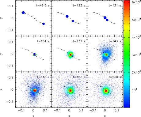
Figure 3: Same as figure 1 for one of the simulations in which the outcome is a direct collision. In particular, this corresponds to the case for which $v_{\rm ini}=120$ km/s and $y_{\rm ini}=0.1R_{\sun}$. [Color figure only available in the electronic version of the article].

In table 1 we list, in addition to the initial parameters of each of the simulations studied here, the outcome of the interaction. When the interaction of the white dwarfs leads to the survival of the eccentric binary we label it as “O”, while when a lateral collision occurs we use “LC” and when the outcome is a direct collision we label the simulation as “DC”. Table 1 also lists for each simulation the total energy of the system, $E$, and its total angular momentum, $L$. Since all the systems studied here have negative energies their initial trajectories are elliptical. Consequently, we also list the perigee ($r_{\min}$) and the apogee ($r_{\max}$) of the initial orbit, and the initial eccentricity. These distances have been calculated using the well-known solution of the two-body problem, assuming that the two white dwarfs are point masses. Namely, we use $\varepsilon=\sqrt{1+(2EL^{2})/(\mu k^{2})}$, where $k=GM_{1}M_{2}$ and $\mu$ is the reduced mass of the system. Finally, we also list $\beta=(R_{1}+R_{2})/r_{\min}$, where $R_{1}$ and $R_{2}$ are the radii of the interacting white dwarfs, which is a parameter which describes the strength of the encounter. Large values of $\beta$ imply large interaction strengths.

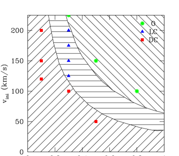
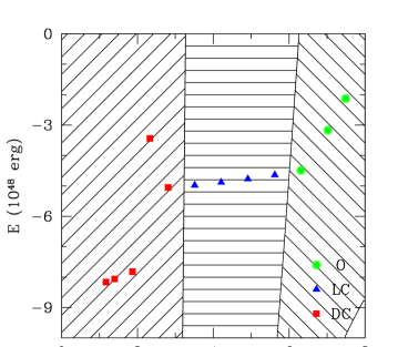
Figure 4: Left panel: regions in the initial velocity-initial distance plane for which the three different outcomes of the white dwarf close encounters occur for the $0.6\,M_{\sun}+0.8\,M_{\sun}$ interaction studied here. The simulations in which a direct collision (DC) occurs are shown using solid squares, solid triangles show the simulations for which a lateral collision (LC) occurs, whilst those in which the binary system survives (O) are represented using solid circles. For sufficiently large initial distancess an eccentric binary system results, while for small initial distances a direct collision happens. In the left and middle shaded regions the outcome is a merger. Right panel: same as the left panel in the energy-angular momentum plane. We emphasize that the transitions between the different regions have been computed using Eqs. (7) to (9), which are valid for point-like masses. [Color figure only available in the electronic version of the article].

A first look at table 1 reveals that the most relevant parameter for discriminating between the three different outcomes previously discussed is the periastron distance, $r_{\min}$, as it should be expected. If the distance at the periastron is smaller than $\simeq 0.033\pm 0.004~{}R_{\sun}$ mass transfer begins and either a lateral collision or a direct one occurs and, thus, a merger turns out to be the unavoidable outcome. However, depending on the exact value of $r_{\min}$ the merger occurs in two or more mass-transfer episodes — for $0.009\pm 0.002~{}R_{\sun}\lesssim r_{\rm min}\lesssim 0.033\pm 0.004~{}R_{\sun}$ — or by means of a direct collision, for $r_{\rm min}\lesssim 0.009\pm 0.002~{}R_{\sun}$.

In figure 4 we show the different outcomes of the interactions as a function of the initial velocities and distances (left panel) and as a function of the total energy and angular momentum of each simulation (right panel). Red squares correspond to simulations in which the final outcome is a direct collision, blue triangles to those in which we obtain a lateral collision and, finally, green circles to those in which an eccentric binary system survives. Finally, the theoretical combinations of initial parameters that lead to the three different outcomes previously discussed are represented in these planes using different shaded regions. The borders of these regions have been obtained using the well-known solution of the two body problem for the periastron distance

$$r_{\min}=\frac{k}{2\mid E\mid}\left(1-\sqrt{1+\frac{2EL^{2}}{\mu k^{2}}}\right)$$ (6)

and imposing, respectively, $r_{\min}=0.033$ and $0.009\,R_{\sun}$. The regions of the left panel of figure 4 have been obtained using the same procedure and taking into account that

$$r_{12} = \left(x_{\rm ini}^{2}+y_{\rm ini}^{2}\right)^{1/2}$$ (7)

$$E = \frac{1}{2}\left(M_{1}+M_{2}\right)v_{\rm ini}^{2}-\frac{GM_{1}M_{2}}{r_{12}}-\frac{1}{2}\left(M_{1}+M_{2}\right){v_{\rm cm}}^{2}$$ (8)

$$= 2\mu v_{\rm ini}^{2}-\frac{G(M_{1}+M_{2})\mu}{r_{12}}$$

$$L = \frac{1}{2}\left(M_{1}+M_{2}\right)v_{\rm ini}y_{\rm ini}$$ (9)

$$+ \left(M_{1}+M_{2}\right)\left(x_{\rm cm}v_{{\rm cm}_{y}}-y_{\rm cm}v_{{\rm cm}_{x}}\right)$$

$$= 2\mu y_{\rm ini}v_{\rm ini}$$

As can be seen, for sufficiently large initial $y$-distances the eccentric binary system survives the interaction, while for small initial distances a direct collision always occurs. Between both regions there exists another one in which a lateral collision occurs.

In all the cases in which a merger occurs the resulting configuration consists of a central white dwarf and a debris region. The morphology of this region will be discussed below. Table 2 lists several important physical quantities. Specifically, for the cases in which a lateral or a direct collision occurs — and, thus, for those cases in which the final result of the interaction is a central white dwarf surrounded by the debris of the collision — we list the mass of the central white dwarf ($M_{\rm WD}$) obtained at the end of the interaction, the mass of the debris ($M_{\rm debris}$) of the collision, and the mass ejected during the interaction ($M_{\rm ej}$). A precise definition of these masses is given in §4.2. Additionally, we list the peak temperature achieved for each simulation, $T_{\rm peak}$ which will be useful when discussing the chemical composition of the remnants, the maximum temperature, $T_{\max}$, of the hot region that we find on top of the primary white dwarf, the radius of the region where the debris of the collisions are found, $R_{\rm debris}$, the total time in which the collision occurs, $\Delta t$, and the nuclear, neutrino and gravitational energies released during the interaction ($E_{\rm nuc}$, $E_{\nu}$, and $E_{\rm GW}$, respectively). The duration of the collision is defined as the time elapsed since mass transfer begins until the system reaches a symmetric configuration. All these quantities are of interest for discussing the structure and nucleosynthesis of the merger remnants.

It is worth noting that for runs 3 to 7 a good fraction of the mass of the less massive white dwarf is accreted onto the more massive white dwarf, thus increasing the total mass of the central remnant. In all these cases the collisions are rather gentle and thus although the interactions result in a merger and occur in dynamical timescales, mass transfer happens during relatively long times (see column 8 of table 2). In the case of runs number 8 and 9 very little mass is accreted by the more massive white dwarf, whereas for runs 10,11 and 12 the collision is so strong that the impact of the less massive white dwarf removes mass from the more massive one and, consequently, the mass of the mass of the central remnant is smaller than that of the original massive white dwarf. Note as well that the mass ejected during the interaction is relatively small in all the cases, of the order of $\sim 10^{-2}\,M_{\sun}$, so the interactions are almost conservative. Consequently, the mass of debris surrounding the central merged object follow a trend reverse of that that described before for the central white dwarf. This behavior can be related to the previously defined interaction strength $\beta$ (see table 1). For runs 3, 4, 5, 6 and 7 we have $\beta=4.00$, 0.54, 0.69 and 0.95, respectively, whilst for runs 10, 11 and 12 we obtain 6.67, 10.0 and 20.0. Clearly, the former runs can be considered as relatively mild, whereas the later are rather strong. However, it is interesting to note that, at odds with what occurs with the debris masses, the size of the regions in which we find the debris of the collisions is totally independent of the kinematical characteristics of the interacting white dwarf ($y_{\rm ini}$ and $v_{\rm ini}$). We emphasize, however, that the density distribution is very different depends very much on these characteristics (see below).

4.2 Structure of the merger remnants

Due to the different dynamics of the white dwarf interactions the resulting merged configurations are not the same. To illustrate this in Fig. 5 we plot the density profiles for a lateral collision (top panel) and a direct collision (bottom panel) in two directions. The solid line depicts the profile along the equatorial plane and the dashed line in the polar direction. As can be seen in figure 5, in the case of a lateral collision we obtain a completely different merged configuration than that obtained in a direct collision. Specifically, the density profiles along the equatorial plane and along the polar direction show that in the case of a lateral collision the result of the interaction is a nearly spherically symmetrical compact object surrounded by an extended disk, whilst in the case of a direct collision the result of the interaction is a central compact object surrounded by a nearly spherical cloud.

Figure 5: Density profiles of the merged configurations at the end of our simulations for the white dwarf interactions shown in figures 2 (top panel) and 3 (bottom panel). The solid lines correspond to the profiles in the equatorial plane, whereas the dashed line are the profiles in the polar direction.

Figure 6: Distributions of the angular velocity — solid lines — at the end of our simulations for the white dwarf interactions shown in figures 2 (top panel) and 3 (bottom panel). See main text for details.

Figure 6 shows the rotational velocities of the merger remnants for the case of a lateral collision (top panel) and a direct collision (bottom panel). For the case of a lateral collision the rotational velocities are plotted as a function of the cylindrical radius and we have averaged the velocities in concentrical cylindrical shells, whereas for the case of a direct collision we have used instead spherical coordinates. For the case of a lateral collision we also show a keplerian profile, using a dashed line. In these figures we have adopted a reference system comoving with the central remnant. To compute the position and velocity of this reference frame we have computed the center of mass of the remnant, as well as its velocity. To this end we only considered those particles of the remnant with densities larger than a certain threshold, which we have chosen $\rho=6.0\times 10^{3}$ g/cm³. As can be seen in the top panel of Fig. 6, corresponding to a lateral collision, the remnant is made of a central compact object (the most massive white dwarf) which rotates as a rigid solid and, on top of it, it can be found a keplerian disk, which is the product of the entanglement of the spiral arm which forms from the disrupted less massive white dwarf. We remind that this entanglement occurs during the second mass-transfer episode — see Fig. 2. Finally, for the case of a direct collision we also obtain that the central region of the remnant rotates with constant angular velocity. Additionally, on top of the central object we find a nearly spherically symmetric cloud in which the tangential velocity has a profile with a $r^{-5/3}$ dependance. This morphology is a direct consequence of the large strength of the collision. In fact, we find that the collision is so strong that the particles of the colliding white dwarfs are well mixed in all the regions of the remnant. However, a cautionary remark is in order here. In particular, the rigid rotation of the merged configurations seen in this figure is indicative that, even though the numerical viscosity may be small, our artificial viscosity prescription is still larger than the correct physical viscosity. Consequently, it is possible that the rigid rotation found in our simulations is not physical, since it is hard to avoid spurious effects from the artificial viscosity for runs that last many dynamical timescales.

The masses of these two regions for all the simulations presented here, as well as the mass ejected in each run, are listed in Table 2. According to the previous discussion the mass of the central white dwarf corresponds to the mass of the region of the remnant which has constant angular velocity. The mass of the ejecta simply corresponds to the mass of those particles which have velocities larger than the local escape velocity in the comoving frame, while the mass of the debris is that of the region in which the particles have either keplerian velocities (in the case of a lateral collision) or which rotate with a profile with slope $r^{-5/3}$ (in the case of a direct collision).

4.3 Temperatures and nucleosynthesis

Run	He	C	O	Ne	Mg	Si	S	Ar
3	$4\times 10^{-9}$	0.4	0.6	$5\times 10^{-5}$	$6\times 10^{-8}$	$3\times 10^{-11}$	0	0
5	0	0.4	0.6	0	0	0	0	0
6	$1\times 10^{-10}$	0.4	0.6	$2\times 10^{-7}$	$6\times 10^{-10}$	$2\times 10^{-13}$	0	0
7	$5\times 10^{-13}$	0.4	0.6	$7\times 10^{-12}$	0	0	0	0
8	$1\times 10^{-9}$	0.4	0.6	$4\times 10^{-5}$	$6\times 10^{-6}$	$1\times 10^{-7}$	$1\times 10^{-10}$	0
9	$2\times 10^{-8}$	0.399	0.599	$7\times 10^{-4}$	$8\times 10^{-5}$	$1\times 10^{-6}$	$2\times 10^{-9}$	$2\times 10^{-13}$
10	$6\times 10^{-8}$	0.398	0.599	$3\times 10^{-3}$	$3\times 10^{-4}$	$4\times 10^{-6}$	$5\times 10^{-9}$	$6\times 10^{-13}$
11	$1\times 10^{-7}$	0.397	0.598	$3\times 10^{-3}$	$3\times 10^{-4}$	$6\times 10^{-6}$	$7\times 10^{-9}$	$1\times 10^{-12}$
12	$2\times 10^{-7}$	0.397	0.598	$4\times 10^{-3}$	$4\times 10^{-4}$	$7\times 10^{-6}$	$8\times 10^{-9}$	$1\times 10^{-12}$

Table 3: Averaged chemical composition (mass fractions) of the heavy rotationally-supported disk (in the case of lateral collisions) or cloud (in the case of direct collisions) obtained by the end of the interaction, for the cases in which a merger is the outcome.

Figure 7: Temperature profiles of the merged configurations at the end of our simulations for the white dwarf interactions shown in figures 2 (top panel) and 3 (bottom panel). In the case of a lateral collision the abscissa is the cylindrical radius, $d$, while in the case of a direct collision we use the spherical radius.

In figure 7 we display the final temperature profiles for our fiducial cases in which a lateral and a direct collision occur, upper and lower panel respectively. These profiles prove that the maximum temperatures occur very close to the edge of the central coalesced white dwarf, in the rapidly rotating regions which we have previously described, and that the maximum temperatures are rather high, in excess of $T\sim 5\times 10^{8}$ K. Note as well that in these figures, as it was done in Fig. 6, we use a logarithmic scale to better display the regions of interest. As can be seen, the central regions of the merger product are practically isothermal, and on top of the relatively cold, degenerate core a region of high temperatures is present. We refer to this region as the hot corona. On top of this region we find the keplerian disk in the case of a lateral collision and a hot spherically symmetric cloud in the case of a direct collision. The boundaries of the hot corona are clearly shown in figure 7 using dashed lines. We also emphasize that for the case of a direct collision, the temperature of the isothermal core is almost three times larger than that obtained in the case of the lateral collision, a direct consequence of the larger interaction strength.

In column 5 of table 2 we show the maximum temperature when the merger process has finished, for those cases in which this is the outcome of the simulation. As can be seen, the maximum temperatures of the hot coronae or cloud previously described increase as the interaction strength ($\beta$) increases, as one should expect, given that in these cases more mechanical energy is transformed into thermal energy. Additionally, in column 6 of table 2 we also list the peak temperature — that is, the maximum temperature — achieved during the entire simulation, $T_{\rm peak}$, for those cases in which a merger is obtained after the interaction. As expected, the peak temperature increases with the strength of the interaction and, consequently, also do the nuclear and neutrino energies released during the interaction — columns 9 and 10 of table 2. These peak temperatures occur during the most violent phases of the close encounter, when mass-transfer from the less massive white dwarf takes place at very high rates. In all the cases studied here the peak temperature is in excess of $T_{\rm peak}\sim 1.6\times 10^{9}$ K, clearly higher than the carbon ignition temperature $T_{\rm ign}\sim 10^{9}$ K, and leads to significant nuclear processing. However, a strong thermonuclear flash does not develop in any of these simulations because, although the temperature in the region where the material of the less massive white dwarf first hits the more massive one increases very rapidly, degeneracy is rapidly lifted, leading to an expansion of the material, which, in turn, quenches the thermonuclear flash. This agrees with the results of Guerrero et al. (2004), Yoon et al. (2007) and Lorén–Aguilar et al. (2009) for the case in which the coalescence of a double white dwarf binary system occurs. Thus, since these high temperatures are only attained during a very short time interval, thermonuclear processing is relatively mild in all simulations. This is not in contradiction with the results of Raskin et al. (2009) and Rosswog et al. (2009), as these authors computed collisions with much larger collision strengths.

Run	He	C	O	Ne	Mg	Si	S	Ar
3	$1\times 10^{-9}$	0.4	0.6	$3\times 10^{-5}$	$3\times 10^{-8}$	$2\times 10^{-11}$	0	0
5	0	0.4	0.6	0	0	0	0	0
6	$8\times 10^{-14}$	0.4	0.6	$1\times 10^{-12}$	0	0	0	0
7	$1\times 10^{-13}$	0.4	0.6	$2\times 10^{-12}$	0	0	0	0
8	$1\times 10^{-11}$	0.4	0.6	$5\times 10^{-8}$	$3\times 10^{-12}$	0	0	0
9	$2\times 10^{-10}$	0.4	0.6	$7\times 10^{-5}$	$8\times 10^{-6}$	$1\times 10^{-7}$	$1\times 10^{-10}$	$1\times 10^{-14}$
10	$2\times 10^{-9}$	0.399	0.599	$2\times 10^{-3}$	$2\times 10^{-4}$	$3\times 10^{-6}$	$3\times 10^{-9}$	$2\times 10^{-13}$
11	$4\times 10^{-9}$	0.398	0.598	$3\times 10^{-3}$	$3\times 10^{-4}$	$4\times 10^{-6}$	$3\times 10^{-9}$	$3\times 10^{-13}$
12	$5\times 10^{-9}$	0.397	0.598	$4\times 10^{-3}$	$3\times 10^{-4}$	$4\times 10^{-6}$	$4\times 10^{-9}$	$4\times 10^{-13}$

Table 4: Averaged chemical composition (mass fractions) of the hot corona obtained by the end of the interaction, for those cases in which the outcome of the interaction is either a lateral or a direct collision.

The chemical composition of the disk or cloud formed as a consequence of the close encounter can be found for all the simulations presented in this paper in table 3. In this table we show, for each of the mergers computed here, the averaged chemical composition (mass fractions) of the heavily rotationally-supported disk or cloud described previously. We do not show the abundances of Ca, Ti, Cr, Fe, Ni and Zn because they are negligible. As it should be expected, the amount of nuclearly processed matter increases for increasing interaction strenghts. Specifically, for the mergers in which in which the interaction strength is small ($\beta\sim 1$) the abundance of Ne is, at most, of the order $10^{-5}$ by mass, while those of Mg and Si are much smaller, and we do not obtain significant amounts of S and Ar. Instead, for the cases in which $\beta\sim 10$ Ne, with a mass abundance of $\sim 10^{-3}$ is rather abundant and we also find significant amounts of Mg, Si, S and Ar. These abundances are in line with those obtained for the coalescence of two white dwarfs in a binary system (Lorén–Aguilar et al. 2009).

In table 4 we list the mass abundances of heavy nuclei in the hot region at the edge of the central white dwarf for the same cases listed in table 3. We find that, at odds which what occurs in the case of the merger of two white dwarfs in a binary system, these abundances are not very different of those obtained for the disk or cloud. The reason for this is that, as explained previously, in the most violent interactions the material of the most massive white dwarf is removed and incorporated into the debris of the interaction. In summary, both the hot corona and the debris disk or cloud are enhanced in Ne and Mg, which are the main products of carbon burning. However, a cautionary remark regarding the chemical compositions of the mergers studied here must be added. White dwarfs are characterized in $\sim 80\%$ of the cases by a thin hydrogen atmosphere of $\sim 10^{-4}\,M_{\sun}$ on top of a helium buffer of $\sim 10^{-2}\,M_{\sun}$. In the remaining $\sim 20\%$ of the cases, the hydrogen atmosphere is absent. Small amounts of hydrogen or helium could indeed change the nucleosynthetic patterns of the hot corona and debris regions in all these cases. Studying this possibility is beyond the scope of this paper and, thus, the changes in the abundances associated to burning of the helium buffer and of the atmospheric hydrogen layer remain to be explored.

4.4 Comparison with other works

In this section we compare our results with those obtained in other recent works, namely those of Rosswog et al. (2009) and Raskin et al. (2009) and with the results of Lorén–Aguilar et al. (2009) for the merger of white dwarfs in binary systems. However we remark that these comparisons should be taken with some care, as the initial conditions adopted here are quite different of those adopted in the above mentioned works.

Rosswog et al. (2009) studied the interaction of two white dwarfs using a variety of stellar masses. Of the cases studied in Rosswog et al. (2009) the most similar one to our choice of masses is that in which the masses of the colliding white dwarfs are $0.6\,M_{\sun}$ and $0.9\,M_{\sun}$. However, we note that in our case the total mass of the system is smaller than Chandrasekhar’s mass, whilst in the case of Rosswog et al. (2009) the total mass of the system exceeds this mass. Rosswog et al. (2009) used parabolic trajectories and, consequently, the velocities of the colliding white dwarfs at first contact are much larger than those obtained here. Hence, shocks are the natural result in their simulations. In our case the simulation that best matches the initial conditions of Rosswog et al. (2009) is run 10, in which $v_{\rm ini}=120$ km/s and $y_{\rm ini}=0.1\,R_{\sun}$, leading to an interaction strength $\beta=20$ — see Table 1 — which is the maximum interaction strength of all our simulations. In both cases the initial separation is similar, being $x_{\rm ini}\sim 3(R_{1}+R_{2})$ in the case of Rosswog et al. (2009) and $x_{\rm ini}\sim 10(R_{1}+R_{2})$ in our case. Nevertheless, and despite the rather different initial conditions, the maximum temperatures obtained in both simulations agree remarkably well. Specifically, we obtain a maximum temperature $T_{\rm peak}\simeq 5.4\times 10^{9}$ K, whereas Rosswog et al. (2009) obtain $T_{\rm peak}\simeq 7.9\times 10^{9}$ K. While the agreement between both sets of simulations in the case of the temperatures is rather good, an essential difference between both works is the central density of the resulting remnants, we obtain a typical density $\rho\sim 10^{7}$ g cm^-3, whilst Rosswog et al. (2009) obtain a density one order of magnitude larger, $\rho\sim 10^{8}$ g cm^-3. As a consequence, the total nuclear energy released (and, hence, the degree of nuclear processing) in the case of Rosswog et al. (2009), $E_{\rm nuc}\sim 10^{50}$ erg, is substantially larger than that obtained here, $E_{\rm nuc}\sim 10^{48}$ erg.

A comparison with the results of Raskin et al. (2009) is somewhat more difficult, as these authors do not provide all the relevant details to which we can compare. In particular, they study the direct collision of two identical white dwarfs of masses $0.6\,M_{\sun}$ at various initial $y$-distances, namely, $y_{\rm ini}=0$, $0.9$ and $1.7\,R_{\sun}$, placed at an initial distance of $x_{\rm ini}=0$, 0.5 amd $0.9\,R_{1}$. The general behaviour of the simulations is in both cases rather similar, and the temperature obtained is, again, similar in both sets of calculations. Specifically, they mention that the peak temperatures achieved during the collisions are in excess of $10^{9}$ K, a value similar to that obtained here.

It is also interesting to compare our results with those obtained in recent simulations of the merger of white dwarfs in binary systems. As mentioned, the most recent works are those of Lorén–Aguilar et al. (2009) and Yoon et al. (2007). Both sets of simulations yield very similar results. In general we find that the characteristics of the collisionally merged products are rather similar to those of the remnants found in those studies. However, there are as well significant differences. For instance, we find that in the most violent collisions the degree of mixing of the chemical products is much larger here than in the case of white dwarf coalescences in a binary system. Also, the final temperatures obtained here are consistent with those obtained in the works of Lorén–Aguilar et al. (2009) and Yoon et al. (2007), but depend sensitively on the interaction strength. In contrast in the merger of white dwarfs in binary systems the interaction proceeds through Roche-lobe overflow, and thus this additional degree of freedom does not exist. Finally the structure of merger products is similar in the case of lateral collisions, whereas for direct collisions we obtain, as already mentioned, a spherical cloud instead of a keplerian disk.

4.5 An interesting case: multiple mass-transfer episodes

Figure 8: Trajectories of the centers of mass of the most massive white dwarf — solid line — and the less massive white dwarf — dashed line — for run number 5, in which several mass-transfer episodes occur.

Run number 5 is an interesting case and deserves further explanations. This particular case corresponds to a case in which the collision is lateral and the initial conditions have been chosen to probe the transition between a lateral collision and the survival at closest approach of a binary system composed of two white dwarfs — see figure 4 and table 1. Specifically, the initial conditions are such that a very gentle interaction is obtained. Note that the interaction strength is in this case $\beta\sim 0.69$. Thus, this is a representative case of those interactions in which several mass-transfer episodes occur. In particular, for this specific simulation we obtain 7 mass-transfer episodes. However, it is important to realize that this number of mass-transfer episodes is actually a lower limit to the real one, as mass transfer is determined by the numerical resolution of the simulations. Figure 8 displays the trajectories of the centers of mass of both white dwarfs during the entire interaction. As can be seen in this figure, both white dwarfs describe initially elliptical trajectories. During the first approach (at $t\simeq 400$ s) both white dwarfs get very close each other, but very little mass is transferred from the less massive white dwarf to the most massive one — see Fig. 9. As a consequence, the less massive white dwarf, although tidally distorted, still preserves its approximate original shape and describes another elliptical orbit. This first approach is followed by 6 more close passages in which both the maximum and the minimum distance between both components decrease. Eventually, during the seventh approach, the less massive white dwarf dissolves and all its remaining mass is removed. As previously discussed (see table 2), very little mass is ejected from the system and, consequently, the final remnant contains most of the mass of the system.

Figure 9: Mass lost by the less massive white dwarf as a function of time for run number 5.

Figure 9 shows the mass lost by the less massive white dwarf, $-\Delta M_{2}$, as a funtion of time. Note that not all this mass is accreted by the most massive white dwarf. As previously discussed, part of this mass is indeed accreted by the most massive one, part goes to form a debris region and a small fraction is ejected from the system. It is worth noting the first very weak mass-transfer episode at $t\simeq 400$ s. Note as well that in subsequent mass-transfer episodes the less massive white dwarf losses an increasing fraction of mass until it is totally disrupted during the seventh closest approach. Similarly, it is also interesting to note that the periods of the elliptical orbits of both white dwarfs decrease for each one of the succesive mass-transfer episodes — see also figure 8. Figure 9 also shows that no mass is transferred between two succesive close approaches. On the contrary, the mass-transfer rate is non zero only during a short fraction of time during the succesive periastrons. That is, all mass-transfer episodes are of very short durations. In fact, the detailed SPH data shows that the less massive white dwarf has an ellipsoidal shape until the last mass transfer episode, during which it becomes totally distorted. This is not the case of the most massive white dwarf, which preserves its initial spherical shape during the entire interaction.

Figure 10: Angular velocities of the interacting white dwarfs for run number 4. The angular velocity of the most massive white dwarf is shown using a solid line, and that of the less massive one is depicted using a dotted line.

Figure 10 provides additional details of the interaction. Specifically, this figure shows that during the entire interaction the white dwarfs become partially synchronized. Obviously, if both white dwarfs were perfectly synchronized there would be a deformation of the less massive one, and this deformation would be always pointing towards the line connecting the centers of mass of both white dwarfs. If the rotation period of the less massive white dwarf were smaller than the orbital period of the system, the tidal deformation would be lagging behind the line connecting both centers of mass, the reverse being also true. Consequently, there would an additional gravitational torque. This torque would have an opposite sense to that of the orbital angular momentum, leading to a perfect synchronization of the system. However, since the synchronization of the interacting white dwarfs occurs mainly during the mass transfer episodes it is clear that synchronization is mainly the result of the accretion stream connecting the less massive white dwarf with the most massive one. Thus, we think that this is indeed a real effect. However, given our treatment of the artificial viscosity, see §2, it is possible as well that, although largely reduced, some shear viscosity could be present during the phases in which no mass transfer occurs and, thus, some synchronization could partially be a spurious effect.

4.6 Gravitational waveforms

Since a sizeable amount of mass is accelerated at considerable speeds during the interaction of the two white dwarfs and since the system presents a large degree of asymmetry, we expect that a considerable amount of gravitational waves should be radiated. It is thus important to characterize which would be the gravitational wave emission of the white dwarf interactions studied here and to assess the feasibility of detecting them.

To compute the gravitational wave pattern, we proceeded as in Lorén–Aguilar et al. (2005). In particular, we used the weak-field quadrupole approximation (Misner et al. 1973). Higher order terms of gravitational wave emission could be included in calculating the strains. These terms include the current-quadrupole and the mass octupole. It has been shown (Schutz & Ricci 2001) that, for the first of these to be relevant, an oscillating angular momentum distribution with a dipole moment along the angular momentum axis is needed. Consequently, in our calculations only the mass octupole should be considered in the best of the cases. Within this approximation, a term close to $v/c\sim 10^{-3}$ would be added to the derived strains. We have found that for the cases studied here is totally negligible, and thus we do not include it.

The three different behaviors found in the previous sections directly translate in the form of the dimensionless strains $h_{+}$ and $h_{\times}$. Examples of the gravitational waves released are shown in figure 11. These gravitational waveforms correspond to the three cases previously described in §4.1 and depicted in figures 1, 2 and 3. Specifically, the top panel shows the gravitational waveforms in the case in which the eccentric binary white dwarf survives. As can be seen, the waveform is perfectly periodic. The middle and bottom panels show, respectively, the waveforms obtained for a lateral collision and a direct collision. In both cases, at early times the system does not radiate gravitational waves because the accelerations are very small. Once the stars sufficiently approach each other, the signal rapidly grows. In the case of a lateral collision — middle panel of figure 11 — the gravitational wave emission presents two peaks, corresponding to the two phases of rapid mass transfer previously discussed. Between these two peaks the structure of the gravitational waveforms is rather complex. There are clearly several small peaks — a behavior which resembles the ring-down phase observed in many mergers of compact objects — superimposed on a monotonous increasing function. This occurs because in a lateral collision, before the final merger, the two interacting white dwarfs describe a few orbits of decreasing separation, in which some mass transfer occurs between the two components of the system. In the case of a direct collision — bottom panel of figure 11 — the signal first grows and then suddenly fades away. Note that a ring-down phase is clearly visible in this case. It is important to point out as well that for all the cases in which a merger occurs the total energy radiated away in the form of gravitational waves is similar, regardless of the interaction strength — see table 2. In particular, for run 3, which has an interaction strength $\beta\sim 4$ the total gravitational wave energy released amounts to $E_{\rm GW}\simeq 4.2\times 10^{40}$ erg, whilst for run 12, with an interaction strength 5 times larger ($\beta\sim 20$), the total gravitational energy radiated is $E_{\rm GW}\simeq 8.3\times 10^{40}$ erg. Finally, for the cases in which the eccentric binary system remains bound the emission of gravitational waves will most likely circularize and shrink their orbits. Once this occurs, the gravitational wave strains will present an almost periodical sinusoidal-like pattern.

Figure 11: Gravitational wave emission from the collision of a $0.6\,M_{\sun}$ and a $0.8\,M_{\sun}$ white dwarfs. The initial distances and velocities are from top to bottom: $y_{\rm ini}=0.6R_{\sun}$ and $v=150$ km/s, $y_{\rm ini}=0.3R_{\sun}$ and $v=175$ km/s and $y_{\rm ini}=0.1R_{\sun}$ and $v=120$ km/s, which lead to the survival of the eccentric binary, a lateral collision and a direct collision, respectively. The dimensionless strains $h_{+}$ (solid lines) and $h_{\times}$ (dashed lines) are measured in units of $10^{-22}$. The source is located at a distance of 10 kpc.

Amongst the three types of gravitational wave signals, only the periodic ones are, in principle, good candidates to be detected by LISA. However, the frequency of the gravitational emission obtained in our simulations lies far from the optimal sensitivity range of LISA. The orbital period of the binary systems is given by

$$\tau^{2}=\frac{\pi^{2}\mu k^{2}}{2E^{3}}$$ (10)

which for the cases studied here is of the order of $5\times 10^{-4}$ Hz. This frequency is far from the optimal LISA frequency band wich lies around $10^{-2}$ Hz. For the gravitational wave emission of these systems to be detectable by LISA, we would need to further decrease the total energy of the system while keeping a high angular momentum in order for the stars to do not collide. That is, the systems should circularize their orbits. It is clear as well that the formation of systems with quasi-circular orbits by gravitational capture is rather unrealistic. The only way in which this could happen is by a fine-tuned energy and angular momentum transfer in the gravitational capture phase, which seems rather unlikely. Thus, in order for this kind of systems to be able to radiate a gravitational signal able to be detected by LISA, orbital circularization is mandatory. If this circularization is mainly driven by the emission of gravitational waves, its time scale will be given by $\tau_{\rm GW}=E/L_{\rm GW}$, where $L_{\rm GW}$ is the luminosity radiated as gravitational waves, which is given by (Peters & Matthews 1963):

$$L_{\rm GW} =\left[\frac{32}{5}\left(\frac{G^{4}}{c^{5}}\right)M_{1}^{2}M_{2}^{2}(M_{1}+M_{2})/a^{5}\right]f(\epsilon)$$ (11)

$$f(\epsilon) =\frac{1+\frac{73}{24}\epsilon^{2}+\frac{37}{96}\epsilon^{4}}{(1-\epsilon^{2})^{7/2}}$$ (12)

Using typical values we obtain $\tau_{\rm GW}\sim 1$ Gyr, which is much smaller than the typical age of a globular cluster. Thus, we expect that most of the systems would have circularized orbits. According to the recent work of Ivanova et al. (2006), a typical cluster of $2\times 10^{5}\,M_{\sun}$ will have at least 3 LISA binaries at any given moment with periods shorter than a thousand seconds. Thus, possibly, some of these binaries could be the result of the systems studied here. However, a direct detection of these collisions is quite unlikely.

4.7 Fallback luminosities

Another potential observational signature of the mergers resulting from the collisions studied here is the emission from the fallback material in the aftermath of some of the close encounters. We have already shown that as a result of the collisions of two white dwarfs in some of the cases studied so far a merger occurs. We have also shown in §4.2 that the structure of the remnants consists in a central compact object surrounded by either a keplerian disk or a spherically symmetric cloud. Most of the SPH particles of the disk or cloud have circularized orbits. However, as it occurs in the mergers of double neutron stars or white dwarfs, some material from the colliding white dwarfs is found to be in highly eccentric orbits as well. After some time, this material will most likely interact with the recently formed disk or cloud. As discussed in Rosswog (2007) the timescale for this is not set by viscous dissipation but, instead, by the distribution of eccentricities. We follow closely the model proposed by Rosswog (2007) and we compute the accretion luminosity obtained from the interaction of the material with high eccentricities with the remnant by assuming that the kinetic energy of these particles is dissipated within the radius of the debris disk or cloud. Our calculations are done in the reference system comoving with the central remnant.

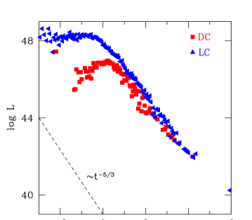
Figure 12: Fallback accretion luminosity for the cases of a direct (DC) and lateral collision (LC). The units of time are seconds, whereas those of luminosities are erg/s. A straight line with slope 5/3 is shown for comparison.

In figure 12 we plot the accretion luminosities as a function of time for the fiducial cases presented in figures 2 and 3. We emphasize that these luminosities have been computed assuming that the highly eccentric particles loose all its kinetic energy when interacting with the disk or cloud, for which we adopt the radius obtained by the end of our SPH simulations and that only a fraction of this energy will be released in the form of high-energy photons. Thus, the results shown in Fig. 12 can be regarded as an upper limit for the actual luminosity of high-energy photons. Note that although the luminosities are smaller than those typically obtained for the merger of double neutron stars — which are typically of the order of $\sim 10^{52}$ erg/s — they are rather high. This is an important result because it shows that observations of high-energy photons can help in detecting the gravitational wave signal radiated by these systems.

It is important to note as well that for direct collisions the slope of the accretion luminosities differ slightly from that obtained in the case of white dwarf mergers ($\propto t^{-5/3}$). The reason for this is the distribution of eccentricities of the accreted particles. We start our discussion noting that in the analytical model of Rosswog (2007) the central object was assumed to be a black hole, whereas we obtain a central massive white dwarf. Moreover, in the model of Rosswog (2007) there are two key parameters, the mass of the central compact remnant and the geometry of the surrounding disk or cloud. Simple numerical experiments reveal that the precise geometry of the disk or cloud only affects to the total radiated energy, whereas the mass of the the central object mainly affects the slope of the fallback luminosity. These dependances are also present in the calculations of Rosswog (2007), see his figure 3. As previously mentioned, in our calculations the central object is a massive white dwarf surrounded by a debris region, not a point-like mass, and, accordingly, we compute the fallback luminosity using the real gravitational potential. Additionally, those particles with very large eccentricities pass very close to the central white dwarf and, thus, feel a gravitational potential of an extended source. On the contrary, and for the same reasons, the gravitational well that those particles with smaller eccentricities feel resembles that of a point-like source. Finally, the particles with large eccentricities reach their periastron at late times because at the end of the merger they are located, on average, at larger distances. Consequently, these particles contribute to the fallback luminosity at late times and the contrary holds for particles with smaller eccentricities. Thus, at late times we expect that the slope of the fallback luminosity will differ from the canonical value of $-5/3$, whilst for early times we expect that the this should be the slope, and this is indeed what we find. As can be seen in figure 12, for $\log t<3$ the slope of the fallback luminosity is $\sim-1.64$, very close to the canonical value, while for $\log t>3$ the fallback luminosity can be best approximated by a $\sim t^{-1}$ curve. Note, however, that for the case of lateral collisions the slope of the accretion luminosity presents the classical $-5/3$ slope. Indeed, in this case the resulting disk is very similar to that obtained in the merger of white dwarfs, and thus in this case the results are very similar.

5 Discussion and conclusions

In this paper we have studied the collisions and close encounters of two white dwarfs, using a state of the art Smoothed Particle Hydrodynamics code. Collisions between two white dwarfs are not as frequent as binary mergers. However, as discussed in Timmes (2009), Rosswog et al. (2009) and Raskin et al. (2009), they most likely occur in globular clusters and the central regions of galaxies, where the stellar densities are very high. The collision time, $\tau_{\rm coll}$, adopting a Maxwellian velocity distribution with dispersion $\sigma$, and assuming a closest approach distance $r_{\min}<2R_{*}$ is (Binney & Tremaine 1987):

$$\frac{1}{\tau_{\rm coll}}=16\sqrt{\pi}n_{\rm WD}\sigma R_{*}^{2}\left(1+\frac{v_{\rm esc}^{2}}{4\sigma^{2}}\right)$$ (13)

where $n_{\rm WD}\simeq 10^{4}$ pc^-3 is the typical number density of white dwarfs in a globular cluster, $v_{\rm esc}\simeq 4000$ km/s is the white dwarf escape velocity and $\sigma\simeq 5$ km/s is the relative velocity dispersion of both white dwarfs in a the globular cluster, which is entirely dominated by gravitational focusing. Consequently, the rate of collisions for a typical globular cluster is given by:

$$r_{\rm GC}\sim\frac{1}{2}\frac{n_{\rm WD}}{\tau_{\rm coll}}\;\frac{4}{3}\pi r_{\rm c}^{3}$$ (14)

where $r_{\rm c}\sim 1.5$ pc is the core radius of the globular cluster (Peterson & King 1975). Adopting the previously mentioned typical values, we obtain $r_{\rm GC}\sim 8\times 10^{-10}$ yr^-1. Taking into account that the density of globular clusters is $n_{\rm GC}=4.2$ Mpc^-3 (Brodie & Strader 2006) as Rosswog et al. (2009) did, we obtain an overall rate of interactions $R\sim 3\times 10^{-10}$ Mpc^-3 yr^-1. Thus, although these interactions are not very frequent, they are not unlikely and, thus, there is a possibility of detecting them.

Motivated by this we have studied the collisions and close encounters of two otherwise typical white dwarfs of masses $0.8$ and $0.6\,M_{\sun}$, respectively, for a broad range of initial conditions and employing a large number of SPH particles. Our initial conditions have been chosen in such a way that a close encounter or a collision is always guaranteed, and are summarized in Table 1. We have found that the outcome of the interactions can be either a direct collision, a lateral collision, in which several mass-transfer episodes may occur, and finally the survival of the eccentric binary system of two white dwarfs. We have characterized the range of initial velocities and distances — or, alternatively, the range of energies and angular momenta — which lead to each one of these outcomes. We find that when the distance between the two white dwarfs at the closest approach is smaller than $0.009\pm 0.002\,R_{\sun}$ the final outcome is a direct collision, when it ranges between $0.009\pm 0.002\,R_{\sun}$ and $0.033\pm 0.004\,R_{\sun}$, the outcome is a lateral collision and otherwise the double degenerate binary system survives.

In all the cases in which a collision is the result of the interaction we obtain that little mass is ejected during the entire merging process and that a central white dwarf surrounded by a debris region is formed. If the collision is direct this region has spherical symmetry, whilst if the collision is lateral we obtain a heavy rotationally-supported keplerian disk. In both cases the peak temperatures achieved during the interaction exceed the carbon ignition temperature and some nucleosynthesis occurs. However, since these high temperatures are not achieved during long periods of time the abundances of heavy nuclei are not large (see tables 3 and 4). Naturally, the extent to which nuclear burning proceeds depends on the strength of the interaction, and hence the production of heavy nuclei is larger in direct collisions. Most of the nuclear reactions occur when matter from the less massive white dwarf is shocked on the surface of the most massive one. Consequently, we find that the maximum temperatures of the merged system occur on a hot corona around the most massive white dwarf.

We have also paid special attention to a specific case of a lateral collision in which several (up to 7) mass-transfer episodes occur. We have found that mass-transfer only occurs during the periastron, and that at each passage the distance between the two interacting white dwarfs decreases, that the mass lost by the less massive white dwarf increases, and that there is substantial synchronization of the system.

We have also computed possible observational signatures of these events. Specifically, we have calculated the emission of gravitational waves and the fallback luminosities in the aftermath of the merger. We have shown that it is very unlikely that LISA will detect the gravitational waves radiated during these interactions. Only at very late phases, when the orbits are circularized, the emission of gravitational waves from those systems in which an eccentric binary is initially formed is possible. However, at these very late stages all the information about the close encounter is completely lost. We have also computed the fallback luminosities which result from those interactions in which a merger occurs. We have found that although these luminosities are somewhat smaller than those obtained in the merger of a binary white dwarf system they are still rather large, allowing the future detection of these events.

Finally, we would like to emphasize that our main aim was to study to the post-capture scenario for a fixed pair of masses of the colliding white dwarfs. Our study differs from those of Rosswog (2009) and Raskin et al. (2009) in the adopted masses of the colliding white dwarfs and in the initial conditions. This is a consequence of the different motivations of all three works. Whereas the studies of Rosswog (2009) and Raskin et al. (2009) were aimed at producing Type Ia supernova outbursts, our work was focused at studying the tidal disruption of typical white dwarfs in globular clusters. For this reason both Rosswog (2009) and and Raskin et al. (2009) studied direct collisions adopting different masses for the colliding white dwarfs than those adopted in this study. Additionally, Rosswog et al. (2009) placed the colliding white dwarfs in a parabolic orbit and, moreover, the total mass of the system was larger than Chandrasekhar’s mass. In this sense, all three studies are complementary but, obviously, more studies are needed to explore the full range of possibilities.

References

- [1] Balsara, D.S., 1995, J. Comp. Phys., 121, 357
- [2] Barnes, J., & Hut, P., 1986, Nature, 324, 446
- [3] Benz, W., 1990, in “The numerical modelling of Nonlinear stellar pulsations”, Ed.: J. Buchler, (Dordrecht: Kluwer Academic Publishers), 269
- [4] Benz, W., Cameron, A.G.W., & Bowers, R.L., 1989, in “White Dwarfs” Proc. of the IAU Coll. 114, Ed.: G. Wegner, Lecture Notes in Physics 328, Springer-Verlag (Berlin) p. 511
- [5] Benz, W., Cameron, A.G.W., Press, W.H., & Bowers, R.L., 1990, A&A, 348, 647
- [6] Benz, W., Thielemann, F.K., & Hills, J.G., 1989, ApJ, 342, 986
- [7] Berger, L., Koester, D., Napiwotzki, R., Reid, I.N., & Zuckerman, B., 2005, A&A, 444, 565
- [8] Brodie, J.P., & Strader, J. 2006, ARA&A, 44, 193
- [9] Charpinet, S., Fontaine, G., & Brassard, P., 2009, Nature, 461, 501
- [10] Clement, M.J., 1974, ApJ, 194, 709
- [11] Davies, M.B., 2002, in “Omega Centauri, A Unique Window into Astrophysics”, Eds: F. van Leeuwen, J.D. Hughes & G. Piotto, ASP Conf. Proc. 265, 215
- [12] Fabian, A.C., Pringle, J.E. & Rees, M.J., 1975, MNRAS, 172, 15
- [13] Freitag, M., & Benz, W., 2005, MNRAS, 358, 1133
- [14] Gingold, R.A., & Monaghan, J.J., 1977, MNRAS, 181, 375
- [15] Guerrero, J., García–Berro, E., & Isern, J., 2004, A&A, 413, 257
- [16] Hernquist, L., & Katz, N., 1989, ApJS, 70, 419
- [17] Hills, J.G., & Day, C.A., 1976, ApJ, 17, L87
- [18] Iben, I., Jr., & Tutukov, A.V., 1984, ApJS, 54, 335
- [19] Itoh, N., Hayashi, H., Nishikawa, A., & Kohyama, Y., 1996, ApJS, 102, 411
- [20] Ivanova, N., Heinke, C.O., Rasio, F.A., Taam, R.E., Belczynski, K., & Fregeau, J., 2006, MNRAS, 372, 1043
- [21] King, A.R., Pringle, J.E., & Wickramasinghe, D.T., 2001, MNRAS, 320, L45
- [22] Lee, H.M., & Ostriker, J.P., 1986, ApJ, 310, 176
- [23] Lorén–Aguilar, P., Guerrero, J., Isern, J., Lobo, J.A., & García–Berro, E., 2005, MNRAS, 356, 627
- [24] Lorén–Aguilar, P., Isern, J., & García–Berro, E., 2009, A&A, 500, 1193
- [25] Lucy, L.B., 1977, AJ, 82, 1013
- [26] Misner, C.W., Thorne, K.S., & Wheeler, J.A., 1973, “Gravitation” (New York: W.H. Freeman)
- [27] Monaghan, J.J., 1997, J. Comp. Phys., 136, 298
- [28] Monaghan, J.J., 2005, Rep. Prog. in Phys., 68, 1703
- [29] Monaghan, J.J., & Gingold, R.A., 1983, J. Comp. Phys., 52, 374
- [30] Monaghan, J.J., & Lattanzio, J.C., 1985, A&A, 149, 135
- [31] Peters, P.C., & Mathews, J., 1963, Phys. Rev., 131, 435
- [32] Peterson, C.J., & King, I.R., 1975, AJ, 80, 427
- [33] Press, W.H., & Teukolsky, S.A., AJ, 1977, 213, 183
- [34] Price, D.J., 2007, PASA, 24, 159
- [35] Rasio, F.A., & Shapiro, S.L., 1995, ApJ, 438, 887
- [36] Raskin, C., Timmes, F.X., Scannapieco, E., Diehl, S., & Fryer, C., 2009, MNRAS, 399, L156
- [37] Rauscher, T., & Thielemann, F.K., 2000, Atom. and Nucl. Data Tabl., 75, 1
- [38] Rosswog, S., 2007, MNRAS, 376, L48
- [39] Rosswog, S., Kasen, D., Guillochon, J., & Ramirez-Ruiz, E., 2009, ApJ, 705, L128
- [40] Ruffert, M., 1992, A&A, 265, 82
- [41] Schutz, B.F., & Ricci, F., 2001, in “Gravitational Waves. One of a Series in High Energy Physics, Cosmology and Gravitation”, Eds.: E. Ciufolini, V. Gorini, U. Moschella, & P. Fré, (Bristol: IOP), 11
- [42] Segretain, L., Chabrier, G., Hernanz, M., García–Berro, E., & Isern, J., 1994, ApJ, 434, 641
- [43] Segretain, L., Chabrier, G., & Mochkovitch, R., 1997, ApJ, 481, 355
- [44] Serna, A., Alimi, J.M., & Chieze, J.P., 1996, ApJ, 461, 884
- [45] Shara, M.M., 2002, “Stellar collisions, mergers and their Consequences”, ASP Conf. Cer. Proc., 263
- [46] Shara, M.M., & Hurley, J.R., 2002, ApJ,571, 830
- [47] Shara, M.M., & Regev, O., 1986, ApJ, 306, 543
- [48] Sills, A., & Bailyn, C.D., 1999, ApJ, 513, 428
- [49] Sills, A., Adams, T., & Davies, M.B., 2005, MNRAS, 358, 716
- [50] Timmes, F.X., 2009, in “SNIa progenitors Workshop 2009”, Ed.: E. Aubourg, online proceedings, (http://sn.aubourg.net/workshop09/pdf/timmes.pdf)
- [51] Timmes, F.X. , & Arnett, D., ApJS, 1999, 125, 277
- [52] Tuchman, Y., 1985, ApJ, 288, 248
- [53] Webbink, R.F., 1984, ApJ, 277, 355
- [54] Willems, B., Kalogera, V., Vecchio, A., Ivanova, N., Rasio, F.A., Fregeau, J.M., & Belczynski, K., 2007, ApJ, 665, L59
- [55] Yoon, S.C., Podsiadlowski, P., & Rosswog, S., 2007, MNRAS, 380, 933