Numerical Evaluation of Shot Noise using Real Time Simulations

Abstract

We present a method to determine the shot noise in quantum systems from knowledge of their time evolution - the latter being obtained using numerical simulation techniques. While our ultimate goal is the study of interacting systems, the main issues for the numerical determination of the noise do not depend on the interactions. To discuss them, we concentrate on the single resonant level model, which consists in a single impurity attached to non-interacting leads, with spinless fermions. We use exact diagonalisations (ED) to obtain time evolution, and are able to use known analytic results as benchmarks. We obtain a complete characterization of finite size effects at zero frequency, where we find that the finite size corrections scale $\propto G^{2}$, $G$ the differential conductance. We also discuss finite frequency noise, as well as the effects of damping in the leads.

The study of current fluctuations in nanodevices such as quantum point contacts and tunnel junctions is deeply connected with some of the most important physical questions. These include the nature of fundamental excitations in strongly interacting electronic systems de Picciotto et al. (1995); Kumar et al. (1996), the possibility of fluctuation theorems out of equilibrium Esposito et al. (2009), and the time evolution of many body entanglement Klich and Levitov (2009a, b). Experimental progress in this area has been swift - second and third cumulants have been measured in several systems Reulet et al. (2003); Bomze et al. (2005), shot noise of single hydrogen molecules have been measured Djukic and van Ruitenbeek (2006), and even the full counting statistics has been obtained in semi conductor quantum dots Gustavsson et al. (2006).

On the theory side, the free case has given rise to a lot of analytical studies Levitov and Lesovik (1993); Levitov et al. (1996); Klich and Levitov (2009a, b), but progress on the most interesting situations - far from equilibrium and with strong interactions - has been difficult (see Gogolin et al. (2007) for a review). Over the years, extensions of the Bethe ansatz to study transport properties have been proposed Fendley and Saleur (1996); Konik et al. (2001); Mehta and Andrei (2008); Chao and Palacios (2010), which might open the road to important progress.

The numerical situation is somewhat similar. $I-V$ characteristics had remained inaccessible until very recently, where methods based on time dependent DMRG have been successfully used to tackle some simple nanostructures Boulat et al. (2008a).

It seems reasonable to expect that time dependent DMRG results could also be used to determine current fluctuations, which could also, in some setups, be determined analytically Saleur and Weiss (2001). In order to reach this ambitious goal, it is crucial to be able to extract cumulants - in particular the shot noise - from real time simulation methods. We propose in this paper a method to do this.

The main problem in the determination of the noise - and the main emphasis of our work - is the finite size analysis of the results of non-equibrium correlation functions for finite systems. To concentrate on this aspect, we only discuss results for the non-interacting resonant level model (RLM) where the numerical data can be obtained using exact diagonalisation (ED) techniques. Since in this specific case there are straightforward analytical solutions of the problem, we can check in great detail the reliability of our approach. We want to emphasize however that the method to be described below is independent of the underlying numerical algorithm, and can therefore also be used in combination with, e.g., time dependent Density Matrix Renormalisation Group (td-DMRG). We will report on this in the case of the interacting resonant level model in a forthcoming paper.

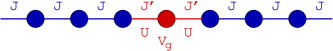
Figure 1: Sketch of the IRLM model. $J^{\prime}$ denotes the coupling of the impurity to the left and right lead, $J$ is the hopping element in the leads, $U$ is the interaction on the contact link, and $V_{\mathrm{g}}$ is a gate voltage. In this work we set $V_{\mathrm{g}}=0$ (the dot level is on resonance), and $U=0$ (non-interacting case, which allows to treat the problem via ED).

We note that prior to our work, a numerical study of the full counting statistics for another non interacting model appeared in Schönhammer (2007). The method used there is however entirely specific to the free case, and uses intermediate analytical results from Levitov and Lesovik (1993). Our approach, in contrast, is based directly on the ‘experimentally’ measured time evolution of the current.

To make things concrete, we start by giving the Hamiltonian of our test system. It is composed of a structure ($\hat{H}_{\mathrm{S}}$) attached to leads ($\hat{H}_{\mathrm{L}}$) described in real space by

$$\hat{H} =\hat{H}_{\mathrm{L}}+\hat{H}_{\mathrm{S}},$$ (1)

$$\hat{H}_{\mathrm{L}} =-J\sum_{m=-\infty}^{-2}\hat{c}^{\dagger}_{m+1}\hat{c}^{\phantom{\dagger}}_{m}-J\sum_{m=1}^{\infty}\hat{c}^{\dagger}_{m+1}\hat{c}^{\phantom{\dagger}}_{m}+\mathrm{h.c.},$$ (2)

$$\hat{H}_{\mathrm{S}} =-J^{\prime}\sum_{m=\pm 1}(\hat{c}^{\dagger}_{m}\hat{c}^{\phantom{\dagger}}_{0}+\hat{c}^{\dagger}_{0}\hat{c}^{\phantom{\dagger}}_{m})+V_{\mathrm{g}}\hat{n}_{0}$$

$$\phantom{=}+U\sum_{m=\pm 1}\Big{(}\hat{n}_{m}-\frac{1}{2}\Big{)}\Big{(}\hat{n}_{0}-\frac{1}{2}\Big{)},~{}~{}\hat{n}=\hat{c}^{\dagger}\hat{c},$$ (3)

cf. Fig. 1. The nearest-neighbour hopping matrix elements in the leads and the coupling of the structure to the leads are given by $J$ and $J^{\prime}$. In the remainder of this work we concentrate on the resonant case at zero gate voltage $V_{\mathrm{g}}=0$ and half filling. Since we want to compare the numerical data with analytical results, we furthermore restrict ourselves to the non-interacting case with $U=0$.

To prepare the system in a state with finite current through the structure, we add a charge imbalance operator $\hat{Q}={V_{\textsc{sd}}}\left(\hat{N}_{\mathrm{L}}-\hat{N}_{\mathrm{R}}\right)/2$ to the Hamiltonian and calculate the initial state as the ground state $|\Psi(t=0)\rangle=|\Psi_{0}\rangle$ of $\hat{H}+\hat{Q}$. Here, $\hat{N}_{\mathrm{L}}$ ($\hat{N}_{\mathrm{R}}$) counts the particle number in the left (right) lead. We then perform the time evolution with the Hamiltonian without $\hat{Q}$. The time evolution is performed by means of the time evolution operator $\hat{U}=\mathrm{e}^{-\mathrm{i}\hat{H}t}$, while all expectation values are evaluated with respect to the initial state $|\Psi_{0}\rangle$. For details see Schmitteckert and Schneider (2006); Schneider and Schmitteckert (2006); Boulat et al. (2008b); Al-Hassanieh et al. (2006); da Silva et al. (2008); Kirino et al. (2008); Heidrich-Meisner et al. (2009); Branschädel and Schmitteckert .

The current operator $\hat{I}_{m}$ for the current at bond $m$ is given by

$$\hat{I}_{m}(t)=\mathrm{i}\frac{e}{\hbar}J_{m}\left[\hat{c}^{\dagger}_{j}(t)\hat{c}^{\phantom{\dagger}}_{j+1}(t)-\hat{c}^{\dagger}_{j+1}(t)\hat{c}^{\phantom{\dagger}}_{j}(t)\right].$$ (4)

We define the current operator as an average over the current on the left and the right contact of the nanostructure

$$\hat{I}(t)=\frac{1}{2}\left[\hat{I}_{-1}(t)+\hat{I}_{0}(t)\right].$$ (5)

The expectation value of $\hat{I}(t)$ in the RLM for $J^{\prime}=0.4J$ and for some values of ${V_{\textsc{sd}}}$ is shown in the upper part of Fig. 2. Effects like the finite settling time $t_{\mathrm{S}}$ and the finite transit time $t_{\mathrm{R}}$ as well as the $I$-${V_{\textsc{sd}}}$-characteristics have been discussed before in great detail Schmitteckert and Schneider (2006); Wingreen et al. (1993); Branschädel and Schmitteckert .

Figure 2: Time dependent current $I(t)$, and current correlation function $S(t,t_{\text{min}})$ with $t_{\text{min}}=12$, in the non-interacting resonant level model RLM, with tight-binding leads and a finite system size of $M=60$ lattice sites, for different values of the bias voltage ${V_{\textsc{sd}}}$. The $I(t)$ curves show the three time regimes given by the settling time $t_{\mathrm{S}}$ and the recurrence time $t_{\mathrm{R}}$. The highlighted time domain indicates the integration range $[t_{\text{min}},t_{\text{max}}]$. The inset demonstrates an additional subtility: the correlation function shows finite size reflection effects on the time scale $t-t_{\mathrm{min}}\gtrsim t_{\mathrm{R}}/2$, which imposes an additional restriction on $t_{\mathrm{max}}$.

Shot noise is defined as the zero-temperature contribution to noise in a transport state. To obtain the noise power spectrum from a real time simulation, the current-current correlations in the time domain

$$S(t,t^{\prime}) =\frac{1}{2}\langle\Delta\hat{I}(t)\Delta\hat{I}(t^{\prime})+\Delta\hat{I}(t^{\prime})\Delta\hat{I}(t)\rangle$$ (6)

$$={\mathrm{Re}}\langle\Delta\hat{I}(t)\Delta\hat{I}(t^{\prime})\rangle$$ (7)

have to be calculated in a non-equilibrium zero-temperature state, where $\Delta\hat{I}(t)=\hat{I}(t)-\langle\hat{I}(t)\rangle$ Landau and Lifshitz (1959); Imry (1997). Therefore, the time dependent expectation value

$$\langle\Delta\hat{I}(t)\Delta\hat{I}(t^{\prime})\rangle=\langle\Psi_{0}|\mathrm{e}^{\mathrm{i}\hat{H}t}\Delta\hat{I}\mathrm{e}^{-\mathrm{i}\hat{H}(t-t^{\prime})}\Delta\hat{I}\mathrm{e}^{-\mathrm{i}\hat{H}t^{\prime}}|\Psi_{0}\rangle$$ (8)

has to be evaluated. In a steady state the correlation function must fulfil $S(t,t^{\prime})\equiv S(t-t^{\prime})$. Then the noise power can be defined as the Fourier transform

$$2\pi\delta(\omega+\omega^{\prime})S(\omega)=\langle\Delta\hat{I}(\omega)\Delta\hat{I}(\omega^{\prime})+\Delta\hat{I}(\omega^{\prime})\Delta\hat{I}(\omega)\rangle,$$ (9)

where

$$S(\omega) =2\int\limits_{-\infty}^{\infty}\mathrm{d}t\,\mathrm{e}^{\mathrm{i}\omega t}S(t,t^{\prime}=0)$$ (10)

$$=4{\mathrm{Re}}\int\limits_{0}^{\infty}\mathrm{d}t\,\mathrm{e}^{\mathrm{i}\omega t}S(t,t^{\prime}=0).$$ (11)

The right-hand side of the equation accounts for the symmetry $S(t-t^{\prime})=S(t^{\prime}-t)$. In a steady state, of course, this expression should be independent of the choice of the time $t^{\prime}$

$$S=4{\mathrm{Re}}\int\limits_{t^{\prime}}^{\infty}\mathrm{d}t\,\mathrm{e}^{\mathrm{i}\omega(t-t^{\prime})}S(t,t^{\prime})~{}~{}~{}\forall\;t^{\prime}.$$ (12)

In the zero-frequency limit $\omega=0$ this expression simplifies to

$$S\equiv S(\omega=0) =4\int\limits_{t^{\prime}}^{\infty}\mathrm{d}t\,S(t,t^{\prime})$$ (13)

$$=4\int\limits_{t^{\prime}}^{\infty}\mathrm{d}t\,{\mathrm{Re}}\langle\Delta\hat{I}(t)\Delta\hat{I}(t^{\prime})\rangle.$$ (14)

We now want to see whether the noise can be reliably obtained in a real time simulation based on this formula.

There are of course many obstacles. The first comes from the calculation of a nonequilibrium correlation function in the time domain from a real time simulation. Because we are restricted to a finite system with $M$ lattice sites and hard walls, a steady transport state is not well defined. Instead, we make the attempt to calculate the time evolution from the initial non-equilibrium state $|\Psi(t=0)\rangle$ as described before and look for a quasi-stationary time regime. The “switching” of a finite source-drain voltage ${V_{\textsc{sd}}}$ at initial time causes a ringing of the current Wingreen et al. (1993), cf. also Fig. 2, which decays exponentially within a settling time $t_{\mathrm{S}}$. The current finally enters a plateau regime, where the size of the plateau is given by the recurrence time $t_{\mathrm{R}}$ which is finite due to the finite size of the system Schneider and Schmitteckert (2006), Fig. 2.

Figure 3: Noise $S$ and squared differential conductance $G^{2}$ for $J^{\prime}=0.4J$. The blue lines represent the analytic values obtained using the Landauer–Büttiker approach. The finite size of the system introduces an additional noise proportional to $G^{2}/M$ (for discussion see text).

Having obtained results for the system “close” to a steady state, to obtain the quantity $S$ we now have to evaluate the integral (14) in a limited time range

$$S_{\mathrm{num}}=4\int\limits_{t_{\mathrm{min}}}^{t_{\mathrm{max}}}\mathrm{d}t\,{\mathrm{Re}}\langle\Delta\hat{I}(t)\Delta\hat{I}(t_{\mathrm{min}})\rangle_{\Psi}$$ (15)

where $t_{\mathrm{min}}>t_{\mathrm{S}}$ and $t_{\mathrm{max}}<t_{\mathrm{R}}$. In a hypothetical situation with a system of infinite size where $t_{\mathrm{R}}\rightarrow\infty$ the contribution of $\int_{t_{\mathrm{max}}}^{\infty}\mathrm{d}t\,{\mathrm{Re}}\langle\Delta\hat{I}(t)\Delta\hat{I}(t_{\mathrm{min}})\rangle_{\Psi}$ can be neglected if ${\mathrm{Re}}\langle\Delta\hat{I}(t)\Delta\hat{I}(t_{\mathrm{min}})\rangle_{\Psi}$ is small for $t>t_{\mathrm{max}}$ as compared to the mean value in the range $t_{\mathrm{min}}<t<t_{\mathrm{max}}$. One therefore has to choose the size of the system big enough to ensure the correlation function to drop to zero within the recurrence time.

The finite recurrence time $t_{\mathrm{R}}$ introduces a finite cutoff frequency $\omega_{\text{cut}}=2\pi/{t_{\mathrm{R}}}\propto 1/M$. This is the main problem we encounter. In contrast to the situation of infinite leads, where zero frequency noise vanishes without applied voltage, we now find a contribution to the zero voltage shot noise of the order of $S(\omega_{\text{cut}})$! The low frequency domain is the most interesting for the kind of problems we wish to study: low frequency is low energy and thus strong coupling between impurity and leads.

Figure 4: Noise $S(\omega)$ vs. frequency $\omega$, both rescaled with respect to the width of the conductance peak $\Gamma=(2J^{\prime}/J)^{2}$, for different values of the bias voltage. The lines going through the numerical values (represented by crosses) are just guides for the eye. The dotted lines correspond to the analytical result for the wide band limit.

The magnitude of the finite size effects for the type of systems that can be studied today is far from negligible. On fig. 3 we give results for the shot noise $S_{\text{num}}$ obtained for different system sizes of $M$ lattice sites, as well as the expected result $S$ in the thermodynamic limit obtained from the Landauer–Büttiker approach (this is discussed in more details in the appendix). Obviously, While the results measured for finite size and the asymptotic results agree at large voltages, there is a marked difference at small voltages, with an offset at vanishing $V_{\text{SD}}$. On the figure, we also represented the finite size correction

$$\Delta S_{\text{num}}=S_{\text{num}}-S$$ (16)

rescaled by the system size $M$. For different values of $M$ the rescaled finite size corrections $M\times\Delta S_{\text{num}}$ collapse very well on a single curve, indicating that the main finite size effects scale linearly with $1/M$ in the considered parameter regime. One may expect that the cut off given by the finite size of the leads corresponds to an effective finite temperature $\sim M^{-1}$ resulting in a low voltage offset $\sim G/M$. However, we find $\Delta S_{\text{num}}\propto G^{2}$ with the differential conductance $G({V_{\textsc{sd}}})=\mathrm{d}I({V_{\textsc{sd}}})/\mathrm{d}{V_{\textsc{sd}}}$.

To understand the behavior of $\Delta S_{\text{num}}$, we consider the full frequency dependence of the shot noise. It can easily be obtained analytically in the wide band limit - see the appendix, Eq. (28). For values of $J^{\prime}/J\ll 1$, the numerical results obtained for the model with cosine dispersion relation should be consistent with the analytical result as long as the considered frequency is small compared to the band width. This is illustrated on fig. 4. There, the frequency dependent noise is obtained via

$$S_{\text{num}}(\omega)=4{\mathrm{Re}}\int\limits_{t_{\text{min}}}^{t_{\text{max}}}\mathrm{d}t\,\mathrm{e}^{\mathrm{i}\omega(t-t_{\text{min}})}S(t,t_{\text{min}})$$ (17)

for different values of the bias voltage ${V_{\textsc{sd}}}$. For big values of $\omega$, the effects of the band curvature are quite marked - as can be seen by the departure of the various guide lines from the dotted lines representing the analytic wide band limit results .

Figure 5: Slope of the frequency dependent shot noise in the limit $\omega\rightarrow 0^{+}$, rescaled to fit with $G^{2}$, for different system sizes. In the low voltage regime we find finite size effects.

To understand the voltage dependency of the finite size corrections, we consider the low frequency behaviour of the analytical results in the wide band limit where we find

$$S(\omega>0,{V_{\textsc{sd}}})=S(0,{V_{\textsc{sd}}})+\Delta S(\omega,{V_{\textsc{sd}}})+\mathcal{O}(\omega^{2})$$ (18)

with the correction in first order with respect to $\omega$

$$\Delta S(\omega,{V_{\textsc{sd}}})\propto G^{2}({V_{\textsc{sd}}})\omega.$$ (19)

For the system with finite band width, we have checked this expression by extracting the slope $\partial S(\omega,{V_{\textsc{sd}}})/\partial\omega$ in the limit $\omega\rightarrow 0^{+}$ from the numerical data. Again we find good agreement with $G^{2}$ in a voltage regime where finite size effects can be neglected, Fig. 5.

Inserting the cutoff frequency now leads to the expression

$$\Delta S(\omega_{\text{cut}},{V_{\textsc{sd}}})\propto\frac{1}{M}G^{2}({V_{\textsc{sd}}})$$ (20)

which is in good agreement with $\Delta S_{\text{num}}({V_{\textsc{sd}}})$, cf. Fig. 3.

Using our knowledge of the finite size correction, we can now control the extrapolation of numerical data: in Fig. 7 we show the results obtained using linear extrapolation $1/M\rightarrow 0$ for $J^{\prime}=0.3J$ and $J^{\prime}=0.4J$. We find indeed very good agreement with the analytical result.

The non-interacting case is of course very simple to calculate numerically (regardless of the possibility of the Landauer–Büttiker treatment). The numerical main effort consists in the exact diagonalisation of the $M\times M$ Hamiltonian matrices as well as the calculation of the time evolution which involves the multiplication of $M\times M$ matrices. Including interaction spoils this approach. Instead, one has to resort to approximative time evolution schemes using methods for correlated electrons. In Branschädel and Schmitteckert we showed that using Wilson leads, or damped boundary conditions (DBC), respectively, with a weak damping constant allows one to effectively increase the system size to $M_{\text{eff}}>M$ lattice sites without changing $M$, where a rough estimate for $M_{\text{eff}}$ has been given as a function of the damping constant $\Lambda$ and the length of the damped leads $M_{\Lambda}$

Figure 6: Noise $S$ and squared differential conductance $G^{2}$ for $J^{\prime}=0.4J$. The blue lines represent the analytic values obtained using the Landauer–Büttiker approach. The system size is fixed to $M=60$ lattice sites, while at the boundaries, the hopping matrix elements are exponentially damped with the damping constant $\Lambda^{-1/2}$ on $M_{\Lambda}$ links. This results in an effectively enlarged system with $M_{\text{eff}}$ lattice sites. The finite size correction $\Delta S_{\text{num}}$, here rescaled by $M_{\text{eff}}$, again collapses on a single curve for different $M_{\text{eff}}$, and is still proportional to $G^{2}$.

$$M_{\text{eff}}\approx M-2M_{\Lambda}+\frac{4}{\ln\Lambda}\big{(}\Lambda^{M_{\Lambda}/2}-1\big{)}.$$ (21)

We now use this estimate to perform the linear extrapolation to infinite system size, where we additionally adjust the estimate by fixing the extrapolated value to analytic results (cf., e.g., Blanter and Büttiker (2000))

$$S({V_{\textsc{sd}}}=0)=0.$$ (22)

To verify this approach we performed calculations for a non-interacting system with $M=60$ lattice sites and DBC, for $J^{\prime}=0.4J$. For the damped leads we used different combinations of $\Lambda$ and $M_{\Lambda}$, where we used values for the damping constant in the range $\Lambda^{-1/2}\in[0.93,1.0]$ for damped leads of $M_{\Lambda}=0\ldots 26$ lattice sites (while keeping the total number of lattice sites $M$ fixed!). The estimate for the effective system size, Eq. (21), is checked by looking at the scaling behaviour of the finite size correction $\Delta S_{\text{num}}$, where we now find linear scaling $\propto 1/M_{\text{eff}}$, cf. Fig. 6.

Figure 7: Shot Noise $S$ as function of the source drain voltage ${V_{\textsc{sd}}}$ in the non-interacting resonant level model. The analytical result was obtained using the Landauer–Büttiker theory, Eq. (27), while the numerical result is computed for systems of different finite sizes of $M=120...180$ lattice sites with a subsequent linear extrapolation of $1/M\rightarrow 0$. The two curves correspond to different couplings $J^{\prime}$ of the impurity to the leads. Furthermore, we used DBC in order to effectively increase the system size. Here, the system size was fixed to $M=60$ lattice sites. For weak damping and for not too big values of ${V_{\textsc{sd}}}$, we find very good agreement with the undamped case.

The result is shown in Fig. 7. We find remarkably good agreement with the analytical result, while we have to point out that, for values of the bias voltage in the order of the band width, the approach fails, which has to be expected since the estimate of the system size only works in a limited voltage range Branschädel and Schmitteckert . Additionally we find the numerical data to be very noisy depending on the respective configuration of the damping conditions.

To conclude, we have introduced a new way of extracting the finite bias shot noise from real time evolution calculations. Very accurate quantitative results are possible as long as finite size effects are treated properly. The possibility of effectively enlarging the system size using Wilson leads has been successfully tested for a limited voltage range. Our results for shot noise in the RLM show very good agreement with results obtained from the Landauer–Büttiker approach for zero as well as finite frequencies. Additionally we confirm a $G^{2}$ dependent scaling of the finite size error in the zero frequnecy regime.

The concept is not restricted to non-interacting fermions and could be implemented using numerical methods for interacting quantum systems. In this case as well, we expect the finite size corrections to go as $1/M$ because the cutoff frequency $\omega_{\text{cut}}$ has the same dependence. We note however that the prefactor might not be $G^{2}(V_{\text{SD}})$ exactly: the jury is still out on the small frequency behavior of the noise in the presence of interactions.Lesage and Saleur (1997); Chamon et al. (1995)

We acknowledge the support by the DFG Center for Functional Nanostructures (CFN), project B2.10.

Appendix A Analytical results

For the non-interacting system in the thermodynamic limit, Eqns. (1-3), with $U=0$, one can derive analytic results for the differential conductance and the shot noise from single particle scattering states. The energy dependent single particle tunneling probability $\tau$ is given as

$$\tau(\epsilon)=\frac{1-\epsilon^{2}/(4J^{2})}{1+(\epsilon-{V_{\mathrm{g}}})\Big{[}(J^{2}-2J^{\prime 2})\epsilon-J^{2}{V_{\mathrm{g}}}\Big{]}/(4J^{\prime 4})}.$$ (23)

Using the Landauer approach (cf., e.g., Blanter and Büttiker (2000)) one obtains for the dc current $I$ and the noise $S$ at zero frequency and for a symmetric voltage drop ${V_{\textsc{sd}}}$

$$I({V_{\textsc{sd}}}) =\int_{-{V_{\textsc{sd}}}/2}^{{V_{\textsc{sd}}}/2}\mathrm{d}\epsilon\,\tau(\epsilon),$$ (24)

$$S({V_{\textsc{sd}}}) =\int_{-{V_{\textsc{sd}}}/2}^{{V_{\textsc{sd}}}/2}\mathrm{d}\epsilon\,\tau(\epsilon)(1-\tau(\epsilon)).$$ (25)

For the resonant case with ${V_{\mathrm{g}}}=0$ this results in

$$G({V_{\textsc{sd}}})=\frac{\partial I}{\partial{V_{\textsc{sd}}}}=\frac{1-{V_{\textsc{sd}}}^{2}/(16J^{2})}{1+{V_{\textsc{sd}}}^{2}(J^{2}-2J^{\prime 2})/(16J^{\prime 4})},\\$$ (26)

$$S({V_{\textsc{sd}}})=\frac{1}{2}\bigg{(}1+\left(\frac{T_{\textsc{b}}}{4J}\right)^{2}\bigg{)}\Bigg{[}T_{\textsc{b}}\bigg{(}1+3\left(\frac{T_{\textsc{b}}}{4J}\right)^{2}\bigg{)}\;\arctan\left(\frac{V}{T_{\textsc{b}}}\right)-V\;\frac{1+3\left(\frac{T_{\textsc{b}}}{4J}\right)^{2}+2\left(\frac{V}{4J}\right)^{2}}{1+\left(\frac{V}{T_{\textsc{b}}}\right)^{2}}\Bigg{]}$$ (27)

where $T_{\textsc{b}}={4J^{\prime 2}}/{\sqrt{J^{2}-2J^{\prime 2}}}$ is a scale. For the frequency dependent noise, we will contend ourselves by giving the result for the wide band limit only:

$$S(\omega,{V_{\textsc{sd}}},T_{\textsc{b}})= \frac{T_{\textsc{b}}}{4}\Theta({V_{\textsc{sd}}}-|\omega|)\Big{\{}\Big{[}\arctan\Big{(}\frac{{V_{\textsc{sd}}}}{T_{\textsc{b}}}\Big{)}+\arctan\Big{(}\frac{{V_{\textsc{sd}}}-2|\omega|}{T_{\textsc{b}}}\Big{)}\Big{]}+\frac{T_{\textsc{b}}}{2\omega}\ln\Big{(}\frac{T_{\textsc{b}}^{2}+({V_{\textsc{sd}}}-2|\omega|)^{2}}{T_{\textsc{b}}^{2}+{V_{\textsc{sd}}}^{2}}\Big{)}\Big{\}}$$

$$+\frac{T_{\textsc{b}}}{4}\Big{\{}\arctan\Big{(}\frac{{V_{\textsc{sd}}}+2|\omega|}{T_{\textsc{b}}}\Big{)}-\arctan\Big{(}\frac{{V_{\textsc{sd}}}-2|\omega|}{T_{\textsc{b}}}\Big{)}\Big{\}},$$ (28)

where in this limit $T_{\textsc{b}}={4J^{\prime 2}\over J}$.

References

de Picciotto et al. (1995)
R. de Picciotto,
M. Heiblum,
H. Shtrikman,
and D. Mahalu,
Phys. Rev. Lett. 75,
3340 (1995).
Kumar et al. (1996)
A. Kumar,
L. Saminadayar,
D. Glattli,
Y. Jin, and
B. Etienne,
Phys. Rev. Lett. 76,
2778 (1996).
Esposito et al. (2009)
M. Esposito,
U. Harbola, and
S. Mukamel,
Rev. Mod. Phys. 81,
1665 (2009).
Klich and Levitov (2009a)
I. Klich and
L. Levitov,
Phys. Rev. Lett. 102,
100502 (2009a).
Klich and Levitov (2009b)
I. Klich and
L. Levitov,
AIP CONFERENCE PROCEEDINGS
1134, 36
(2009b).
Reulet et al. (2003)
B. Reulet,
J. Senzier, and
D. Prober,
Phys. Rev. Lett. 91,
196601 (2003).
Bomze et al. (2005)
Y. Bomze,
G. Gershon,
D. Shovkun,
L. Levitov, and
M. Reznikov,
Phys. Rev. Lett. 95,
176601 (2005).
Djukic and van
Ruitenbeek (2006)
D. Djukic and
J. M. van Ruitenbeek,
Nano Letters 6,
789 (2006).
Gustavsson et al. (2006)
S. Gustavsson,
R. Leturcq,
B. Simovic,
R. Schleser,
T. Ihn,
P. Studerus, and
K. Ensslin,
Phys. Rev. Lett. 96,
076605 (2006).
Levitov and Lesovik (1993)
L. Levitov and
G. Lesovik,
JETP Lett 58,
230 (1993).
Levitov et al. (1996)
L. Levitov,
H. Lee, and
G. B. Lesovik,
J. Math. Phys. 37,
4845 (1996).
Gogolin et al. (2007)
A. Gogolin,
R. Konik,
A. W. W. Ludwig,
and H. Saleur,
Ann. der Physik 16,
678 (2007).
Fendley and Saleur (1996)
P. Fendley and
H. Saleur,
Phys. Rev.B 54,
10845 (1996).
Mehta and Andrei (2008)
P. Mehta and
N. Andrei,
Phys. Rev. Lett. 100,
086804 (2008).
Konik et al. (2001)
R. Konik,
A. W. W. Ludwig,
and H. Saleur,
Phys. Rev. Lett. 87,
236801 (2001).
Chao and Palacios (2010)
S. P. Chao and
G. Palacios
(2010), eprint cond-mat/1003.5395.
Boulat et al. (2008a)
E. Boulat,
H. Saleur, and
P. Schmitteckert,
Phys. Rev. Lett. 101,
140601 (2008a).
Saleur and Weiss (2001)
H. Saleur and
U. Weiss,
Phys. Rev. B 62,
201302 (2001).
Schönhammer (2007)
K. Schönhammer,
Phys. Rev. B 75,
205329 (2007).
Schmitteckert and
Schneider (2006)
P. Schmitteckert
and
G. Schneider, in
High Performance Computing in Science and
Engineering ’06, edited by W. E.
Nagel,
W. Jäger,
and M. Resch
(Springer, Berlin,
2006), pp. 113–126.
Schneider and
Schmitteckert (2006)
G. Schneider and
P. Schmitteckert
(2006), eprint cond-mat/0601389.
Boulat et al. (2008b)
E. Boulat,
H. Saleur, and
P. Schmitteckert,
Physical Review Letters 101,
140601
(2008b).
Al-Hassanieh et al. (2006)
K. A. Al-Hassanieh,
A. E. Feiguin,
J. A. Riera,
C. A. Büsser,
and E. Dagotto,
Physical Review B (Condensed Matter and Materials Physics)
73, 195304
(2006).
da Silva et al. (2008)
L. G. G. V. D. da Silva,
F. Heidrich-Meisner,
A. E. Feiguin,
C. A. Büsser,
G. B. Martins,
E. V. Anda, and
E. Dagotto,
Physical Review B (Condensed Matter and Materials Physics)
78, 195317
(2008).
Kirino et al. (2008)
S. Kirino,
T. Fujii,
J. Zhao, and
K. Ueda,
Journal of the Physical Society of Japan
77, 084704
(2008).
Heidrich-Meisner
et al. (2009)
F. Heidrich-Meisner,
A. E. Feiguin,
and E. Dagotto,
Phys. Rev. B 79,
235336 (2009).
(27)
A. Branschädel
and
P. Schmitteckert, eprint arXiv:1004.4178.
Wingreen et al. (1993)
N. S. Wingreen,
A. P. Jauho, and
Y. Meir,
Phys. Rev. B 48,
8487 (1993).
Landau and Lifshitz (1959)
L. D. Landau and
E. M. Lifshitz,
Statistical Physics (Pergamon,
Oxford, 1959).
Imry (1997)
Y. Imry,
Introduction to Mesoscopic Physics
(Oxford University Press, 1997).
Blanter and Büttiker (2000)
Y. M. Blanter and
M. Büttiker,
Physics Reports 336,
1 (2000).
Lesage and Saleur (1997)
F. Lesage and
H. Saleur,
Nucl. Phys. B 490,
543 (1997).
Chamon et al. (1995)
C. Chamon,
D. Freed, and
X. Wen,
Phys. Rev. B 51,
2363 (1995).