Adiabatic quantum computation: Enthusiast and Sceptic’s perspectives

Enthusiast’s abstract

Enthusiast’s perspective: We analyze the effectiveness of AQC for a small rank problem Hamiltonian $H_{F}$ with the arbitrary initial Hamiltonian $H_{I}$. We prove that for the generic $H_{I}$ the running time cannot be smaller than $O(\sqrt{N})$, where $N$ is a dimension of the Hilbert space. We also construct an explicit $H_{I}$ for which the running time is indeed $O(\sqrt{N})$. Our algorithm can be used to solve the unstructured search problem with the unknown number of marked items.

Sceptic’s perspective: We show that for a robust device, the running time for such $H_{F}$ cannot be much smaller than $O(N/\ln N)$.

Overture.—Adiabatic quantum computation (AQC) (e.g. FGGS ) is a Hamiltonian -based model of quantum computation. The idea behind AQC is that finding the ground state of a problem Hamiltonian $H_{F}$ solves interesting computational problems. In the abstract setting, let $H_{I}\,,H_{F}$ be a pair of hermitian $N\times N$ matrices, with $N\gg 1$. Consider the interpolating Hamiltonian $H(s)$ of the form

$$H(s):=(1-f(s))H_{I}+f(s)H_{F}\,,$$ (1)

where $f$ is a monotone function on $[0,1]$ satisfying $f(0)=0$, $f(1)=1$. We will denote by $P_{I}$ (respectively $P_{F}$) the spectral projection on the ground state energy $E_{I}$ ($E_{F}$) of the matrix $H_{I}$ ($H_{F}$). We prepare the initial state of the system $\psi(0)$ in the (a-priori known) ground state $\psi_{I}\in Range\,P_{I}$ of the Hamiltonian $H_{I}$ range , and let the system evolve according to the (scaled) Schrödinger equation:

$$i\dot{\psi}_{\tau}(s)\ =\ \tau H(s)\psi_{\tau}(s)\,,\quad\psi_{\tau}(0)\ =\ \psi_{I}\,.$$ (2)

The adiabatic theorem of quantum mechanics ensures that under certain conditions the evolution $\psi_{\tau}(1)$ of the initial state stays close to the $Range\,P_{F}$. For AQC to be a potent quantum algorithm, the running (i.e. physical) time $\tau$ in Eq. (2) must be much smaller than $N$. Although AQC attracted a considerable interest in physics and computer science communities, the quantitative characterization of the speed up in its use remains at large unknown. The core issue here is related to the extreme sensitivity of the adiabatic behavior to the spectral structure of the operator $H(s)$. Specifically, the deviations may become large when the gap $g(s)$ between the ground state of $H(s)$ and the rest of its spectrum is small in the vicinity of some instant $s\in[0,1]$.

The traditional approach to the problem so far was to estimate this minimal gap rema . Putting a few rare exceptions aside (e.g. DMV ), it is usually a very hard task. This explains why, generally speaking, not much light was shed on the effectiveness of AQC. Let us note that the estimates of the running time involving the gap $g(s)$ alone provide only the upper bound on the optimal running time $\tau$. In reality $\tau$ can be much smaller.

In this paper, we discuss the reliable upper and lower bounds on the optimal value of $\tau$, circumventing the estimates on the size of the gap. Our method is applicable for a particular class of problem Hamiltonians, satisfying the following hypothesis.

Assumption 1.

The problem Hamiltonian is of the small rank: $Rank(H_{F}):=m\ \ll N$.

Even in this narrower context, there is no unequivocal riposte to whether AQC is indeed efficient, as we shall see. As often happens in theoretical deliberations, the answer depends, to some extent, on the degree of your zeal. To keep the discussion balanced, we present two different perspectives: The first one is on the optimistic side while the second one is rather pessimistic in its nature. To this end we set a stage for two close acquaintances, Messrs. Enthusiast and Sceptic, and let the wise Reader judge who of them is closer to the mark.

Let us note that for AQC to work, it suffices to ensure that $\psi_{\tau}(1)$ has a non trivial overlap with the range of $H_{F}$, which we will encode in the requirement $\|P_{F}\psi_{\tau}(1)\|\geq 1/5$, remar . Another issue that usually arouses certain degree of confusion, which we want to avoid, is a normalization of $H(s)$. To that end, we will use the calibration $\|H_{I}\|=\|H_{F}\|=1$. One should bear this convention in mind when performing comparison with other results.

The rest of the paper is organized as follows: We first present the discussion from Enthusiast and Sceptic’s points of view, indicating briefly the intuition behind the corresponding assertions. We then give proofs of Theorems 3 and 4 (the rest of the proofs can be found in CE ). Now we pass the baton to Mr. Enthusiast.

Enthusiast’s perspective.—To formulate the result, let me introduce a set of the related parameters. First, I want to quantify the overlap between the initial state $\psi_{I}$ and the problem Hamiltonian. Namely, let $\delta_{1}=\|H_{F}\psi_{I}\|$, let $\delta_{2}=\|P_{F}\psi_{I}\|$, and let $\delta_{3}=\|Q_{F}\psi_{I}\|$, where $Q_{F}$ is a projection onto $Range\,H_{F}$. Note that for a generic $H_{I}$ all $\delta$’s are small, with $\delta_{1}$ and $\delta_{3}$ being $O(\sqrt{m/N})$, while $\delta_{2}=O(\sqrt{m^{\prime}/N})$. Here $m^{\prime}$ is a dimension of $Range\,P_{F}$. Second, I want to distinguish between $E_{F}$ and the rest of the spectrum of $H_{F}$, which I will assume henceforth are separated by the gap $g_{F}$. Finally, since I don’t want to assume that $H_{F}$ is sign definite and given that $\|H_{F}\|=1$ by convention, the energy $E_{F}$ will show up in the estimates. The prototypical example covered by our results is the generalized unstructured search (GUS) problem, which can be cast in the following form: Suppose $H_{F}$ is diagonal with the unknown number of entries equal to $-1$ and the rest of the entries equal to zero (so that $H_{F}={\bf 1}-P_{F}$). Pick $H_{I}=-|\psi_{I}\rangle\langle\psi_{I}|$ with $\psi_{I}=N^{-1/2}(1,\ldots,1)$. Then the corresponding parameters are $\delta_{3}=\delta_{2}=\sqrt{m/N}$, $E_{F}=-1$, and $g_{F}=1$.

The pair of results below, coupled together, gives fairly tight lower and respectively upper bounds on the optimal running time in AQC.

Theorem 1.

Consider the interpolating family Eq. (1) with an arbitrary $f$. Then the running time $\tau_{-}$ in Eq. (2) for which $\|Q_{F}\psi_{\tau_{-}}(1)\|\geq 1/5$ satisfies

$$\tau_{-}\ \geq\ \frac{1-5\delta_{2}}{5\delta_{1}}\,,\quad\mbox{ for }\quad\delta_{2}<1/5\,.$$ (3)

The quantitative measure of how much $\psi_{\tau}(s)$ deviates from $\psi_{I}$ is encoded in the size of the commutator $[P_{I},H(s)]$. Hence one expects to see the deviation from $\psi_{I}$ over the time $\tau$ such that $\tau\cdot\|[P_{I},H(s)]\|=O(1)$. Since $P_{I}$ commutes with $H_{I}$ while $\|[P_{I},H_{F}]\|\leq 2\delta_{1}$, we get $\|[P_{I},H(s)]\|\leq 2\delta_{1}$ for all $s$ and the bound in Eq. (3) follows up to a constant.

Let me note that the similar, albeit less sharp (with the wrong dependence on $m$) lower bound was recently established in IM .

Theorem 2.

Suppose $\delta_{3}/g_{F}=O(1/\ln N)$, Then there exists an explicit rank one $H_{I}$ and an explicit function $f$ such that $\|P_{F}\psi_{\tau_{+}}(1)\|\ \geq\ 1/5$ for

$$\tau_{+}\ =\ \frac{C(1-E_{F})}{|E_{F}|\,\delta_{2}}\,,$$ (4)

for any $C\in[1/3,2/3]$.

For $N\gg m$ the requirement on $\delta_{3}/g_{F}$ is typically satisfied. Note also that $\tau_{-}/\tau_{+}\approx\sqrt{m^{\prime}/m}$. This is not particularly surprising, as in Theorem 1 the aim was to ensure that $\psi_{\tau_{-}}(1)$ has an overlap with the range of $H_{F}$, whereas in Theorem 2 we want $\psi_{\tau_{+}}(1)$ to overlap with $Range\,P_{F}$.

The choices in the theorem are: $H_{I}=-|\psi_{I}\rangle\langle\psi_{I}|$ and a (non adiabatic) parametrization $f(s)$ is given by

$$f(s)\ =\ \begin{cases}&0\,,\hskip 48.36958pts=0\\ &\alpha\equiv\frac{1}{1-E_{F}}\,,\quad s\in(0,1)\\ &1\,,\hskip 48.36958pts=1\end{cases}\,.$$

That means we move diabatically (instantly) to the given point of the path, stay there for the time $\tau_{+}$, and then move quickly again to the end of the path. Such $f$ is in fact optimal for the Grover’s problem.

The intuition behind this assertion is as follows: With the above choice for $f(s)$

$$\psi_{\tau}(1)\ =\ e^{-i\alpha\tau_{+}\cdot(E_{F}P_{I}\,+\,H_{F})}\psi_{I}.$$

Note now that the ground state energy of $E_{F}P_{I}$ matches that of $H_{F}$ and differs from the energies of its excited states. Let $X$ be a subspace spanned by vectors in the ranges of $P_{I}$ and $P_{F}$, and let $X^{\perp}$ be its orthogonal complement (so that $X\bigoplus X^{\perp}$ is the whole Hilbert space). As usual in adiabatic setting, the transitions between $X$ and $X^{\perp}$ are suppressed due to fast oscillations caused by the energy differential. Therefore the initial state $\psi_{I}$ slowly precesses in the $X$ subspace, and by choosing the right value for $\tau_{+}$ one can find the evolved state sufficiently close to $Range\,P_{F}$. The argument identical to the one in Theorem 1 shows that the running time $\tau_{+}$ is roughly

$$\frac{1-E_{F}}{|E_{F}|}\cdot\frac{1}{\|[P_{I},P_{F}]\|}\,=\,\frac{1-E_{F}}{|E_{F}|}\cdot\frac{1}{2\delta_{2}}\,.$$

Since the precession is very slow, $\tau_{+}$ is fairly robust.

This assertion can be seen as an extension of the classical result of Farhi–Gutmann FG on the Grover’s search problem. For GUS the parallel result was established for the quantum circuit model (QCM) in BHT .

Theorem 2 uses values of $E_{F}$ and $\delta_{2}=\|P_{F}\psi_{I}\|=O(1/\sqrt{N})$ as the input. In many important applications (such as GUS) the value of $\delta_{2}$ is unknown. To this end, we prove the following assertion.

Theorem 3.

Suppose that the value of $E_{F}$ is known. Then there is a Hamiltonian – based algorithm that determines $\delta_{2}$ with $1/N^{2}$ accuracy and requires $O((\ln N)^{2})$ of the running time.

Note that the combined running time in Theorems 2 and 3 remains $O(\sqrt{N})$. The algorithm used in the proof is inspired by the mean ergodic theorem and makes use of the fact that the survival probability $c_{F}(t)=\langle\psi_{I}|e^{itH_{F}}\psi_{I}\rangle$ is directly measurable in AQC framework. For GUS this problem is known as quantum counting and was analyzed in QCM framework in BHT .

Enthusiast’s summary.—Theorem 1 tells us that for a generic $H_{I}$ the running time cannot be smaller than $O(\sqrt{N})$. Theorems 2 and 3 construct the explicit $H_{I}$ and the parametrization $f(s)$ so that $\tau=O(\sqrt{N})$. I have assumed that the ground state energy $E_{F}$ of $H_{F}$ is known with the $1/N$ accuracy.

Sceptic’s perspective.—Let me first point out two shortcomings of the method which is usually employed in estimation of the running time of AQC (e.g. DMV for the Grover’s problem and RKHLZ ). The technique hinges on a choice of a parametrization $f$ such that $\dot{f}(s)$ is small whenever the instantaneous spectral gap $g(s)$ is small rem1 . To construct such $f$, one need to know the values $s_{j}$ for which $g(s_{j})=O(N^{-1/2})$ with high precision. Such analysis requires the detailed information about the spectral structure of $H_{F}$. The similar issue is present (albeit to a lesser extent) in the Enthusiast’s approach, as one still needs to know $E_{F}$. Even if this technical hurdle can be overcome, the extreme susceptibility of $\psi_{\tau}(1)$ to the parametrization $f$ poses a radical problem in practical implementation. Indeed, it is presumably extremely difficult to enforce $\dot{f}=0$ for a long stretch of the physical time, as the realistic computing device inevitably fluctuates. So in the robust setting one can assume that for any given moment $s_{0}$ the value $\dot{f}(s_{0})$ is greater than some small but fixed $\kappa$. We can then as well consider the functions $f$ in the robust setting that satisfy $\dot{f}(s)>\kappa$ for all values of $s$.

To understand how the robust system evolves, let me consider the following semi-empiric argument, substantiated in Theorem 4 below. One can show CE that for a finite rank matrix $H_{F}$ the minimum value $g$ of the gap $g(s)$ between the ground state energy $E(s)$ of $H(s)$ and the rest of the spectrum of $H(s)$ is $O(\delta_{3})$. Let $g=g(s_{0})$, then one can introduce two different time scales: $\tau_{1}$ and $\tau_{2}$. We set $\tau_{1}=\Delta^{-1}$, where $\Delta$ is a gap between the two smallest eigenvalues of $H(s_{0})$ and the rest of its spectrum. The scale $\tau_{2}$ is associated with a two level system corresponding to the restriction of the Hilbert space to the spectral subspace of these two eigenvalues. Typically, $\tau_{1}\ll\tau_{2}$, and $\psi_{\tau}$ stays close to the ground state provided $\tau\gg\tau_{2}$. If $\tau_{1}\ll\tau\ll\tau_{2}$, then $\psi_{\tau}$ will still stay close to the range of the above spectral subspace. However, it will behave as if the avoided level crossing is a true level crossing, with evolution following the first excited state rather than the ground state (see Figure 1).

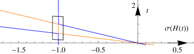
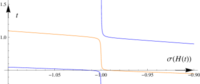
Figure 1: Illustration for Theorem 4, $N=10^{4}$. Top: A pair of relevant eigenvalues of $H(t):=H_{I}+2tH_{F}$ as a function of $t$, for $H_{F}=-\lvert e_{1}\rangle\langle e_{1}\rvert-\frac{1}{2}\lvert e_{2}\rangle\langle e_{2}\rvert$ and $H_{I}=\lvert\phi_{1}\rangle\langle\phi_{1}\rvert-\lvert\phi_{2}\rangle\langle\phi_{2}\rvert$. Here $e_{1}=(1,0\ldots,0)$, $e_{2}=(0,1,0,\ldots,0)$, $\phi_{1}=1/\sqrt{N}(1,\cdots,1)$, and $\phi_{2}=1/\sqrt{N}(1,\ldots,1,-1,\ldots,-1)$, with exactly half of $-1$ so that $\langle\phi_{1}|\phi_{2}\rangle=0$. Bottom: The magnified region of the avoided crossings in the upper panel.

To estimate $\tau_{2}$ let me consider a two level system of the form

$$K(s)\ =\ \left[\begin{array}[]{cc}1-f(s)&\delta f(s)\\ \delta f(s)&f(s)\\ \end{array}\right]\,.$$ (5)

Assuming that $f$ is differentiable, the Landau–Zener formula shows that for $K(s)$ the corresponding time scale is $\tau_{2}\approx\dot{f}(s_{0})\,\delta^{-2}$. The value of the minimal gap here is equal to $\delta\sqrt{1+\delta^{2}}\approx\delta$. Since for $H(s)$ the value of $g$ is roughly $\delta_{3}$, we see that $\psi_{\tau}$ stays close to the ground state of $H(s)$ only if

$$\tau\ >\ \dot{f}(s_{0})\cdot(\delta_{3})^{-2}\ =\ \dot{f}(s_{0})\cdot O(N)\,.$$

Hence in the robust setting, where $\dot{f}$ cannot be too small at any given instant, there is no significant speed up in using AQC. The result below reaffirms this argument for the case of the initial Hamiltonian $H_{I}$ of the small rank. In what follows, $Q_{I}$ will denote the projection onto $Range\,H_{I}$, with $\delta:=\|Q_{I}Q_{F}\|$.

Theorem 4 (Robust lower bound on the running time).

Suppose that $f$ in Eq. (1) is differentiable and satisfies $\dot{f}(s)\geq\kappa>0$ for $s\in[0,1]$. Then, if $\tau<\tau_{r}=O\left(\frac{-\kappa}{m^{2}\delta^{2}\,\ln\delta}\right)$, we have

$$\left|\langle\psi_{I}|\psi_{\tau}\rangle\right|\ >\ \frac{2\sqrt{6}}{5}\,+\,\delta\,.$$ (6)

Hence the running time $\tau$ for which $\|Q_{F}\psi_{\tau}(1)\|\geq 1/5$ cannot be smaller than $\tau_{r}$.

Sceptic’s summary.—Theorem 4 tells us that for a generic $H_{I}$ of the small rank the robust running time $\tau_{r}$ cannot be smaller than $O(N/\ln N)$. Hence AQC is not really effective for the problem Hamiltonians that satisfy Assumption 1.

Proof of Theorem 3.

The starting point is a pair of identities, GR :

$$e^{-p}\sum_{k=1}^{\infty}\frac{p^{k}\sin(k\omega)}{k!} = e^{p(\cos\omega-1)}\sin(p\sin\omega)$$

$$e^{-p}\sum_{k=1}^{\infty}\frac{p^{k}\cos(k\omega)}{k!} = e^{p(\cos\omega-1)}\cos(p\sin\omega)\,.$$ (7)

In particular, if $1-\cos\omega>\Delta$, each term in Eq. (Proof of Theorem 3.) is bounded by $e^{-p\Delta}$ and therefore is smaller than $1/N^{2}$ provided $p=2\ln N/\Delta$. On the other hand, the remainders to the partial sums (up to $k=L$) in Eq. (Proof of Theorem 3.) are $O(p^{L}/L!)$ provided the latter quantity is small. Combining these observations, we get

$$e^{-p}\sum_{k=1}^{p}\frac{p^{k}e^{ik\omega}}{k!}\,=\,\begin{cases}&1+O(1/N^{2})\,,\quad\omega=0\\ &O(1/N^{2})\,,\quad 1-\cos\omega>\Delta\end{cases}\,,$$

for $p=2\ln N/\Delta$ and $\Delta<1$. Hence

$$e^{-p}\sum_{t=1}^{p}\frac{p^{k}}{k!}\,\langle\psi_{I}|e^{it(H_{F}-E_{F})}\psi_{I}\rangle\,=\,(\delta_{2})^{2}+O(1/N^{2})\,,$$ (8)

for $p=2\ln N/(1-\cos g_{F})$. The total running time is $\sum_{t=1}^{p}t=O((\ln N)^{2})$. ∎

Proof of Theorem 4.

For a solution $\psi_{\tau}(s)$ of (2), let

$$\phi_{\tau}(s):=\ e^{ih(s)\tau\,E_{I}}\psi_{\tau}(s)\,,\ h(s)=\int_{0}^{s}(1-f(r))\,\mathrm{d}r\,.$$ (9)

Then one can readily check that $\phi_{\tau}(s)$ satisfies IVP

$$i\dot{\phi}_{\tau}(s)\ =\ \tau\hat{H}(s)\phi_{\tau}(s)\,,\quad\phi_{\tau}(0)\ =\ \psi_{I}\,,$$ (10)

where $\hat{H}(s)=(1-f(s))\,(H_{I}-E_{I})\,+\,f(s)\,H_{F}$. Clearly $\left|\langle\psi_{I}|\psi_{\tau}\rangle\right|=\left|\langle\psi_{I}|\phi_{\tau}\rangle\right|$. Let

$$B(s)=\left(f(s)H_{F}-((1-f(s))E_{I}+\epsilon i\right))^{-1}\,,$$

and let $\phi(s)=\psi_{I}-f(s)H_{F}B(s)\,\psi_{I}$, where $\epsilon$ is a small parameter to be chosen later. Omitting the $s$ dependence, we have

$$\hat{H}\phi=-f(1-f)H_{I}H_{F}B\,\psi_{I}+i\epsilon fH_{F}B\,\psi_{I}\,.$$ (11)

That means that away from the $m$ values of $s$ for which $B(s)$ has zero eigenvalue, $\|\hat{H}\phi\|$ is very small, since $\|H_{I}H_{F}\psi_{I}\|\leq\delta^{2}$. Note now that

$$\langle\phi(1)|\phi_{\tau}(1)\rangle\ =\ \langle\phi(0)|\phi_{\tau}(0)\rangle\,+\,\int_{0}^{1}\frac{d}{ds}\langle\phi(s)|\phi_{\tau}(s)\rangle\,ds\,.$$ (12)

But $\langle\phi(0)|\phi_{\tau}(0)\rangle=1$ and

$$\left|\langle\phi(1)|\phi_{\tau}(1)\rangle\right| = \left|\langle\psi_{I}|\phi_{\tau}(1)\rangle\,-\,\langle\psi_{I}|\frac{H_{F}}{H_{F}-\epsilon\,i}|\phi_{\tau}(1)\rangle\right|$$

$$\leq\ \left|\langle\psi_{I}|\phi_{\tau}(1)\rangle\right|\,+\,\|Q_{F}\psi_{I}\|\ \leq\ \left|\langle\psi_{I}|\phi_{\tau}(1)\rangle\right|\,+\,\delta\,.$$

Substitution into Eq. (12) gives

$$1\,-\,\left|\langle\psi_{I}|\phi_{\tau}(1)\rangle\right|\ \leq\ \left|\int_{0}^{1}\frac{d}{ds}\langle\phi(s)|\phi_{\tau}(s)\rangle\,ds\right|\,+\,\delta\,.$$

Hence Eq. (6) will follow if

$$\left|\int_{0}^{1}\frac{d}{ds}\langle\phi(s)|\phi_{\tau}(s)\rangle\,ds\right|\ <\ 1\ -\ \frac{2\sqrt{6}}{5}\,-\,2\delta\,.$$ (13)

We have

$$\frac{d}{ds}\langle\phi(s)|\phi_{\tau}(s)\rangle\ =\ \langle\dot{\phi}(s)|\phi_{\tau}(s)\rangle\,-\,i\tau\langle\phi(s)|\hat{H}(s)|\phi_{\tau}(s)\rangle\,.$$

We bound the first term on the right hand side by $\|\dot{\phi}\|$ and the second one by $\tau\|\hat{H}\phi_{\tau}\|$. A straightforward computation (using Eq. (11) for the second term) shows that

$$\|\dot{\phi}\|\ \leq\ \frac{\dot{f}\delta}{\Delta_{\epsilon}}\,+\,\frac{2\dot{f}\delta}{\left(\Delta_{\epsilon}\right)^{2}}\,;\ \|\hat{H}\phi_{\tau}\|\ \leq\ \frac{\delta^{2}+\epsilon\delta}{\Delta_{\epsilon}}\,,$$

where $\Delta_{\epsilon}(s):={\,\rm dist}(f(s)\sigma(H_{F})\,,\,(1-f(s))E_{I}+\epsilon\,i)$. Here ${\,\rm dist}(S,z)$ is an Euclidean distance from the set $S$ to the point $z$ in $\mathbb{C}$, and $\sigma(H)$ stands for the spectrum of $H$.

As a result, we obtain a bound

$$\left|\dot{\overbrace{\langle\phi|\phi_{\tau}\rangle}}\right|\ \leq\ (\dot{f}+\tau\delta+\tau\epsilon)\frac{\delta}{\Delta_{\epsilon}}\,+\,2\frac{\dot{f}\delta}{\left(\Delta_{\epsilon}\right)^{2}}\,.$$

Integrating both sides over $s$ and using the bounds

$$\int_{0}^{1}\frac{\dot{f}ds}{\Delta_{\epsilon}(s)} \leq -2m\ln\epsilon\,;\quad\int_{0}^{1}\frac{\dot{f}ds}{\left(\Delta_{\epsilon}(s)\right)^{2}}\ \leq\ \frac{2m}{\epsilon}\,;$$

$$\int_{0}^{1}\frac{ds}{\Delta_{\epsilon}(s)} \leq -2m\frac{\ln\epsilon}{\kappa}\,,$$

we can estimate

$$\left|\int_{0}^{1}\frac{d}{ds}\langle\phi(s)|\phi_{\tau}(s)\rangle\,ds\right|\\ \leq\ 2m\delta\left(-\ln\epsilon\left(1+\frac{\tau\delta}{\kappa}+\frac{\tau\epsilon}{\kappa}\right)+\frac{2}{\epsilon}\right)\,.$$

Hence the required bound in Eq. (13) follows with the choice $\epsilon=10^{-3}m\delta$, provided $\tau\leq-\frac{C\kappa}{\epsilon^{2}\ln\epsilon}$ where $C$ is a constant. ∎

Partially supported by the NSF Grant DMS–0907165.

References

• (1) E. Farhi et al., Science 292, 472 (2001).
• (2) The range of the operator $A$ on a Hilbert space $X$ is a collection of all vectors $y$ such that $y=Ax$ for some $x\in X$. The rank of $A$ is a dimension of $Range\,A$ and coincides with the number of non zero eigenvalues for hermitian $A$. For example, for $A=|\psi\rangle\langle\psi|$ the range consists of vectors proportional to $\psi$ and $Rank\,A=1$.
• (3) We will relate our results with the prior gap-free bounds on $\tau$ (namely IM ; FG ) in the next section.
• (4) W. van Dam et al., 42nd IEEE Symposium on Foundations of Computer Science 279 (2001).
• (5) In fact, it suffices to have an overlap of order $1/p(\ln N)$ , where $p(x)$ is a polynomial in $x$.
• (6) Z. Cao and A. Elgart, arXiv:1004.4911v1.
• (7) L. M. Inannou and M. Mosca, Int. J. Quant. Inform. 6, 419 (2008).
• (8) E. Farhi and S. Gutmann, Phys. Rev. A 57, 2403 (1998)
• (9) G. Brassard et al., Lecture Notes in Comput. Sci. 1444, 820 (Springer-Verlag, New York/Berlin (1998)).
• (10) A. T. Rezakhani et al., Phys. Rev. Lett. 103, 080502 (2009).
• (11) In fact, the Enthusiast’s approach brings this strategy to its extreme by choosing $\dot{f}(s)=0$ for all $s\in(0,1)$. One can show CE that that for the sign definite $H_{F}$ the number of avoided crossings is exactly equal to $m$.
• (12) I. S. Gradshteyn and I. M. Ryzhik, formulae (1.449), Table of integrals, series, and products (Elsevier/Academic Press, Amsterdam, 2007).