Tuning the effects of Landau-level mixing on anisotropic transport in quantum Hall systems

Abstract

Electron-electron interactions in half-filled high Landau levels in two-dimensional electron gases in a strong perpendicular magnetic field can lead to states with anisotropic longitudinal resistance. This longitudinal resitance is generally believed to arise from broken rotational invariance, which is indicated by charge density wave (CDW) order in Hartree-Fock calculations. We use the Hartree-Fock approximation to study the influence of externally tuned Landau level mixing on the formation of interaction induced states that break rotational invariance in two-dimensional electron and hole systems. We focus on the situation when there are two non-interacting states in the vicinity of the Fermi level and construct a Landau theory to study coupled charge density wave order that can occur as interactions are tuned and the filling or mixing are varied. We examine in detail a specific example where mixing is tuned externally through Rashba spin-orbit coupling. We calculate the phase diagram and find the possibility of ordering involving coupled striped or triangular charge density waves in the two levels. Our results may be relevant to recent transport experiments on quantum Hall nematics in which Landau-level mixing plays an important role.

I Introduction

The integerVonKlitzing and fractionalStormer quantum Hall effects have been studied extensively in two-dimensional electron systems (2DES).PrangeGirvin It has been proposedHLR ; MooreRead and observedWillett that the states at half odd integer filling fraction in low Landau levels (LLs) have distinct behaviour from states at odd denominator filling fractions. This distinction extends to higher LLs, where anisotropic transport has been observed at half odd integer filling fractions,Lilly ; Pan ; Lilly2 which is believed to arise from broken rotational symmetry due to electron-electron interactions.FPA ; MoessnerChalker ; KFS ; FKS ; Fogler ; FradkinKivelson ; Yang ; MacDonaldFisher ; FKMN ; Dorsey1 ; Dorsey2 ; Barci ; Doan ; FradkinReview The experimental evidence for broken rotation symmetry at half odd integer filling fractions is large peaks in the longitudinal resistivity, which vanish as the direction of applied current is rotated by ninety degrees.

Hartree-Fock calculations of the effects of electron-electron interactions in high Landau levels indicated a transition to a striped charge density wave (CDW) phase at half odd integer filling fractions.MoessnerChalker ; KFS ; FKS ; Fogler It has been argued by Fradkin and Kivelson and others that the anisotropy is evidence of an electronic nematic phase.FradkinKivelson ; FKMN ; Dorsey1 ; Dorsey2 ; Barci ; Doan ; FradkinReview However there continues to be debate as to whether the states are electronic nematics or smectics.FradkinReview ; recentTsui ; Ciftja

There have been several recent experiments on two-dimensional electron or hole systems that are in or close to the regime where anisotropic quantum Hall states are expected for which Landau level mixing is believed to be either appreciable or tunable via an external parameter.Manfra ; Gusev ; Grayson LL mixing can arise from a variety of sources, such as disorder, geometric confinement effects in a quantum well, interactions or spin-orbit couplingWinklerBook but has generally been ignored in theoretical studies of anisotropic quantum Hall states.FradkinKivelson ; KFS ; MoessnerChalker ; FPA A couple of exceptions are investigations of the effects of LL mixing from electron-electron interactionsMacDonald or disorderStanescu on CDW formation which may be relevant for experiments showing re-entrant behaviour of quantum Hall states in the lowest LL.Csathy There has also been recent interest in LL mixing in the context of non-Abelian quantum Hall states.Simon ; Nayak ; Chesi

We investigate the effects of Landau level mixing on the formation of quantum Hall states with broken rotation symmetry by using the Hartree-Fock approximation to study CDW formation in a two-dimensional system of charged fermions (electrons or holes) when LL mixing and interactions are present. This neglects quantum and thermal fluctuations,Dorsey1 but can be hoped to be as informative as Hartree-Fock studies on single Landau levels.MoessnerChalker ; KFS We assume that there is a term in the Hamiltonian that mixes LLs, leading to non-interacting single-particle eigenstates that are linear combinations of LLs. We explore the effects of interactions on CDW ordering within these eigenstates. We specialize to the situation when two energy levels lie close to the Fermi energy, $E_{F}$, of the system, which can lead to competition between CDW phases of various symmetries originating in different non-interacting states. To study this, we construct a Landau theory for CDW ordering in the presence of LL mixing when there are two states that are close to the Fermi energy. In the range of energies where the two states are close to degenerate we also consider the possibility of quantum Hall ferromagnetism, but for the example we consider here, CDW ordering occurs at higher temperatures within the Hartree-Fock approximation.

In order to study the effects of LL mixing on CDW formation experimentally in a systematic way, some external tuning parameter that can mix LLs is required. Neither disorder nor interactions are particularly suitable for this task. However, Rashba spin-orbit coupling can be tuned experimentally in a quantum well by parameters such as applied gate voltage. This motivates us to investigate the phase diagram as a function of filling fraction, LL mixing and temperature when LLs are mixed via Rashba spin-orbit coupling when two states are relatively close to the Fermi level. We find that at half-integer filling fractions there can be triangular CDW ordering in both levels simultaneously when the filling of the higher energy level is non-zero.

This paper is organized as follows. In Sec. II we investigate electron-electron scattering in the presence of LL mixing in high LLs, using a similar approach to Moessner and Chalker,MoessnerChalker to argue that there is still an instability towards CDW ordering in the presence of LL mixing. In Sec. III we construct a Landau theory for striped and triangular CDW order when there are two states close to the Fermi energy. In Sec. IV we display numerically calculated phase diagrams for LL mixing due to Rashba spin orbit coupling and also discuss possible quantum Hall ferromagnetism near degeneracy. We discuss our results and their possible connection to experiment in Sec. V.

II Interactions in the presence of Landau level mixing

We consider fermions (electrons or holes) confined to two dimensions in a perpendicular magnetic field. We label single-particle basis states as $\left|nkj_{z}\right>$, where $n$ labels LL index, $k$ is the pseudomomentum, and $j_{z}$ is the spin eigenvalue. The projection of the orbital part of the eigenstates onto real-space is the LL wavefunction

$$\psi_{k}^{\left(n\right)}\left(\mathbf{r}\right) = \frac{1}{\sqrt{2^{n}n!\sqrt{\pi}l_{0}L}}e^{iky}\phi_{n}\left(\frac{x-kl_{0}^{2}}{l_{0}}\right),$$ (1)

where we work in the Landau gauge $\mathbf{A}\left(\mathbf{r}\right)=B\left(-y,0,0\right)$, with $L$ the spatial extent of the system and $l_{0}=\sqrt{h/eB}$ the magnetic length.

We assume that there is some source of mixing of the basis states, such as spin-orbit coupling, which leads to a set of non-interacting single-particle eigenstates of the form

$$\left|\Phi k\right> = \sum_{\alpha=\{n_{\alpha},j_{z}^{\alpha}\}}C_{\Phi\alpha}\left|\alpha k\right\rangle,$$ (2)

where the $C_{\Phi\alpha}$ are the coefficients of the basis states and $\left|\alpha k\right\rangle$ is shorthand for $\left|n_{\alpha}kj_{z}^{\alpha}\right\rangle$.

We now allow for interactions between fermions via a potential $V\left(\mathbf{r}\right)$, which has Fourier transform $\tilde{V}\left(\mathbf{q}\right)$, leading to the interaction Hamiltonian

$$H_{I} = \frac{1}{2}\sum_{\left\{\Phi_{1},\Phi_{2},\Phi_{3},\Phi_{4}\right\}}\sum_{\left\{k_{1},k_{2},k_{3},k_{4}\right\}}a_{\Phi_{1}k_{1}}^{\dagger}a_{\Phi_{2}k_{2}}^{\dagger}a_{\Phi_{3}k_{3}}a_{\Phi_{4}k_{4}}$$ (3)

$$\hskip 42.67912pt\times\int\frac{\mbox{d}^{2}\mathbf{q}}{\left(2\pi\right)^{2}}\tilde{V}\left(\mathbf{q}\right)\left\langle\Phi_{1}k_{1};\Phi_{2}k_{2}\left|e^{i\mathbf{q}\cdot\left(\mathbf{r_{2}-r_{1}}\right)}\right|\Phi_{3}k_{3};\Phi_{4}k_{4}\right\rangle$$

$$= \frac{1}{2}\sum_{\left\{\Phi_{1},\Phi_{2},\Phi_{3},\Phi_{4}\right\}}\sum_{\left\{k_{1},k_{2},k_{3},k_{4}\right\}}a_{\Phi_{1}k_{1}}^{\dagger}a_{\Phi_{2}k_{2}}^{\dagger}a_{\Phi_{3}k_{3}}a_{\Phi_{4}k_{4}}\sum_{\alpha\beta\sigma\rho}C_{\Phi_{1}\alpha}^{*}C_{\Phi_{2}\sigma}^{*}C_{\Phi_{3}\rho}C_{\Phi_{4}\beta}\delta_{j_{z}^{\alpha}-j_{z}^{\beta}+j_{z}^{\gamma}-j_{z}^{\delta}}$$

$$\hskip 42.67912pt\times\int\frac{\mbox{d}^{2}\mathbf{q}}{\left(2\pi\right)^{2}}\tilde{V}\left(\mathbf{q}\right)\left\langle n_{\alpha}k_{1}\left|e^{-i\mathbf{q}\cdot\mathbf{r_{1}}}\right|n_{\beta}k_{4}\right\rangle\left\langle n_{\sigma}k_{2}\left|e^{i\mathbf{q}\cdot\mathbf{r_{2}}}\right|n_{\rho}k_{3}\right\rangle,$$

where $a_{\Phi k}$ is the annihilation operator of $\left|\Phi k\right>$, and the four single particle states involved in the interaction are labelled $\left\{\Phi_{1},\Phi_{2},\Phi_{3},\Phi_{4}\right\}$ with corresponding pseudomomenta $\left\{k_{1},k_{2},k_{3},k_{4}\right\}$. The orbital matrix elements have been evaluated by Raikh and ShahbazyanRaikh to be

$$\left\langle n_{\alpha}k_{1}\left|e^{-i\mathbf{q}\cdot\mathbf{r_{1}}}\right|n_{\beta}k_{2}\right\rangle = \frac{2\pi}{L}\delta\left(k_{1}-k_{2}-q_{y}\right)A_{n_{\alpha}n_{\beta}}\left(\frac{1}{2}q^{2}l_{0}^{2}\right)e^{i\left[\frac{1}{2}l_{0}^{2}q_{x}(k_{1}+k_{2})+\left(n_{\alpha}-n_{\beta}\right)\left(\theta-\frac{\pi}{2}\right)\right]},$$

where

$$A_{n_{\alpha}n_{\beta}}\left(x\right) = \left(\frac{n_{\alpha\beta}^{{}^{\prime}}!}{n_{\alpha\beta}!}\right)^{\frac{1}{2}}x^{\frac{\Delta n_{\alpha\beta}}{2}}e^{-\frac{x}{2}}\mathcal{L}_{n_{\alpha\beta}^{{}^{\prime}}}^{\Delta n_{\alpha\beta}}\left(x\right),$$

with $n_{\alpha\beta}=\max\left(n_{\alpha},n_{\beta}\right)$, $n_{\alpha\beta}^{{}^{\prime}}=\min\left(n_{\alpha},n_{\beta}\right)$, $\Delta n_{\alpha\beta}=\left|n_{\alpha}-n_{\beta}\right|$, and $\theta=\arctan\left(q_{y}/q_{x}\right)$. Equation (3) can be rewritten as

$$H_{I} = \frac{1}{2}\sum_{\{\Phi_{1},\Phi_{2},\Phi_{3},\Phi_{4}\}}\sum_{klm}M_{\{\Phi_{1},\Phi_{2},\Phi_{3},\Phi_{4}\}}\left(m,l\right)a_{\Phi_{1}k+l}^{\dagger}a_{\Phi_{2}k+m}^{\mbox{\mbox{ }}\dagger}a_{\Phi_{3}k+l+m}^{\mbox{ }}a_{\Phi_{4}k}^{\mbox{ }},$$ (5)

where

$$M_{\{\Phi_{1},\Phi_{2},\Phi_{3},\Phi_{4}\}}\left(m,l\right) = \sum_{\alpha\beta\sigma\rho}C_{\Phi_{1}\alpha}^{*}C_{\Phi_{2}\sigma}^{*}C_{\Phi_{3}\rho}C_{\Phi_{4}\beta}\mathbf{}\delta_{\alpha\beta}\delta_{\sigma\rho}I_{\alpha\sigma\rho\beta}\left(m,l\right),$$ (6)

and

$$I_{\alpha\sigma\rho\beta}\left(m,l\right) = \frac{2\pi}{L}\int\frac{\mbox{d}^{2}\mathbf{q}}{\left(2\pi\right)^{2}}\tilde{V}\left(q\right)\delta\left(q_{y}-l\right)A_{n_{\alpha}n_{\beta}}\left(\frac{1}{2}q^{2}l_{0}^{2}\right)A_{n_{\sigma}n_{\rho}}\left(\frac{1}{2}q^{2}l_{0}^{2}\right)$$ (7)

$$\hskip 42.67912pt\times e^{-il_{0}^{2}q_{x}m}e^{i\left(\theta-\frac{\pi}{2}\right)\left(n_{\alpha}-n_{\beta}+n_{\sigma}-n_{\rho}\right)}.$$

The function $M_{\{\Phi_{1},\Phi_{2},\Phi_{3},\Phi_{4}\}}\left(m,l\right)$ describes the strength of the interaction between the eigenstates $\Phi_{1},\Phi_{2},\Phi_{3},$ and $\Phi_{4}$ (illustrated in Fig. 1), with the function $I_{\alpha\sigma\rho\beta}\left(m,l\right)$ describing the overlap between the orbital part of the basis states. The strength of the interactions between particular eigenstates can be tuned by using external parameters to vary the coefficients, $C_{\Phi_{i}\alpha}$.

Figure 1: Interaction between states $\Phi_{1}$, $\Phi_{2}$, $\Phi_{3}$, and $\Phi_{4}$. $k$, $l$, and $m$ are pseudomomenta.

II.1 Hartree-Fock Approximation

We now investigate the self-energy and two particle scattering vertex using the Hartree-Fock approximation. Moessner and Chalker MoessnerChalker showed that for fermions interacting with the hard-core potential $\tilde{V}(q)=-vq^{2}$ within a single LL, the Hartree-Fock approximation is exact in the limit of large LL index. We generalize this result to electrons with different LL indices interacting via a hard-core interaction. Provided the difference in LL index is much less than the maximum LL index, then in the limit that the maximum LL index is large, the Hartree-Fock approximation is asymptotically exact for the hard-core potential. We return to consider Coulomb interactions in Sec. III.

To take the large-LL limit, we follow Moessner and Chalker and replace $A_{n_{\alpha}n_{\beta}}(x)$ by its WKB envelope:

$$A_{n_{\alpha}n_{\beta}}\left(x\right) = \frac{1}{\sqrt{\pi}}\left[\frac{n^{\prime}_{\alpha\beta}!}{\left(n^{\prime}_{\alpha\beta}+\Delta n_{\alpha\beta}\right)!}\right]^{1/2}\frac{1}{\left[4n^{\prime}_{\alpha\beta}x-\left(x-\Delta n_{\alpha\beta}\right)^{2}\right]^{1/4}}.$$ (8)

The envelope is defined for $x_{-}^{\alpha\beta}<x<x_{+}^{\alpha\beta}$, where

$$x_{\pm}^{\alpha\beta} = \left(2n_{\alpha\beta}^{\prime}+\Delta n_{\alpha\beta}\right)\left[1\pm\sqrt{1-\left(\frac{\Delta n_{\alpha\beta}}{\Delta n_{\alpha\beta}+2n_{\alpha\beta}^{\prime}}\right)}\right].$$

We now turn to the properties of the interaction vertex $M_{\{\Phi_{1},\Phi_{2},\Phi_{3},\Phi_{4}\}}$ in the limit of large LLs; specifically, we study the properties of function $I_{\alpha\sigma\rho\beta}\left(m,l\right)$ [Eq. (7)]. The function $I_{\alpha\sigma\rho\beta}\left(m,l\right)$ gives the strength of the interaction between eigenstates in terms of the constituent basis states. For the single-particle and two-particle vertices, we focus on the situation when there are two eigenstates lying near the Fermi level.

Substitution of Eq. (8) into Eq. (7) yields

$$I_{\alpha\sigma\rho\beta}\left(m,l\right) = \frac{4}{Ll_{0}}\left[\frac{n^{\prime}_{\alpha\beta}!}{\left(n^{\prime}_{\alpha\beta}+\Delta n_{\alpha\beta}\right)!}\right]^{1/2}\left[\frac{n^{\prime}_{\sigma\rho}!}{\left(n^{\prime}_{\sigma\rho}+\Delta n_{\sigma\rho}\right)!}\right]^{1/2}\int_{q_{x}^{{\rm min}}}^{q_{x}^{{\rm max}}}\frac{\mbox{d}q_{x}}{2\pi}$$

$$\times\frac{\tilde{V}\left(q_{x},l\right)\cos\left[l_{0}^{2}q_{x}m-\left(n_{\alpha}-n_{\beta}+n_{\sigma}-n_{\rho}\right)\left(\arctan\left(\frac{l}{q_{x}}\right)-\frac{\pi}{2}\right)\right]}{\left[8n^{\prime}_{\alpha\beta}\left(q_{x}^{2}+l^{2}\right)-\left(q_{x}^{2}+l^{2}-2\frac{\Delta n_{\alpha\beta}}{l_{0}^{2}}\right)^{2}\right]^{1/4}\left[8n^{\prime}_{\rho\sigma}\left(q_{x}^{2}+l^{2}\right)-\left(q_{x}^{2}+l^{2}-2\frac{\Delta n_{\rho\sigma}}{l_{0}^{2}}\right)^{2}\right]^{1/4}}.$$

As the eigenstates in the presence of LL mixing are not Landau levels, when we refer to the large-LL limit, we mean that the non-interacting single-particle eigenstates near the Fermi energy are dominated by contributions from Landau levels with large indices. If $\Delta n_{\alpha\beta}\neq 0$, and $\Delta n_{\alpha\beta}\ll n^{\prime}_{\alpha\beta}$, then

$$\sqrt{\frac{n^{\prime}_{\alpha\beta}!}{(n^{\prime}_{\alpha\beta}+\Delta n_{\alpha\beta})!}}\sim\left(\frac{1}{n^{\prime}_{\alpha\beta}}\right)^{\frac{\Delta n_{\alpha\beta}}{2}}\to 0$$

as $n^{\prime}_{\alpha\beta}\to\infty$, which causes the interaction vertex $I_{\alpha\sigma\rho\beta}\left(m,l\right)$ to vanish. Thus, in this limit, $I_{\alpha\sigma\rho\beta}\left(m,l\right)$ is finite only when $\Delta n_{\alpha\beta}=\Delta n_{\sigma\rho}=0$, in which case

$$I_{\alpha\sigma\rho\beta}\left(m,l\right) = \frac{4}{Ll_{0}}\delta_{n_{\alpha},n_{\beta}}\delta_{n_{\sigma},n_{\rho}}\int_{0}^{q_{x}^{{\rm max}}}\frac{dq_{x}}{2\pi}\frac{\tilde{V}\left(q_{x},l\right)\cos\left[l_{0}^{2}q_{x}m\right]}{\sqrt{q_{x}^{2}+l^{2}}\left[8n{}_{\alpha}-\left(q_{x}^{2}+l^{2}\right)\right]^{1/4}\left[8n_{\sigma}-\left(q_{x}^{2}+l^{2}\right)\right]^{1/4}},$$

where

$$q_{x}^{{\rm max}} = \sqrt{\left(q^{{\rm max}}\right)^{2}-l^{2}},$$

$$q^{{\rm max}} = {\rm\max}\left\{\sqrt{8n_{a}},\sqrt{8n_{\sigma}}\right\}.$$

If $n_{\alpha}=n_{\sigma}$, the envelopes in Eq. (LABEL:eq:Ideltanzero) associated with $n_{\alpha}$ and $n_{\sigma}$ overlap exactly, whereas when $n_{\alpha}\neq n_{\sigma}$ there is less than perfect overlap, so $I_{\alpha\alpha\alpha\alpha}(m,l)$ will be an upper bound on the interaction vertex.

Let ${\mathcal{N}}$ denote the index of the highest LL basis state that contributes to occupied non-interacting eigenstates. Moessner and Chalker showed that for a contact potential $I_{\alpha\alpha\alpha\alpha}(m,l)$ is non-zero only when $m=0$ in the large-LL limit, hence, as we have established that $I_{\alpha\alpha\alpha\alpha}(m,l)$ is an upper bound for $I_{\alpha\sigma\rho\beta}\left(m,l\right)$, it follows that $I_{\alpha\sigma\rho\beta}\left(m,l\right)$ is nonzero only when $m=0$, and obeys the bound

$$-\sum_{q_{y}}I_{\alpha\sigma\rho\beta}\left(0,q_{y}\right) \leq \frac{2v{\mathcal{N}}}{\pi}.$$

Thus, in the large-LL limit, only exchange terms are important in the interactions between basis states for a contact potential. The results of MC for other classes of diagrams can also be applied here as an upper bound to other types of diagrammatic contributions. Thus, diagrams with crossed interaction lines and closed fermion loops vanish in the large-LL limit. When we consider the case where the relevant constituent LL indices are not necessarily large, we apply the Hartree-Fock approximation directly. In this situation, both Hartree terms and Fock terms are important.

To avoid divergence of the bound on $I_{\alpha\sigma\rho\beta}$ as the number of constituent basis states increases, we scale $v$ with $\mathcal{N}$ such that $v\mathcal{N}$ is constant. Assuming that each eigenstate $\Phi$ is a linear combination of $\mathcal{P}$ LL basis states (for example for Rashba spin-orbit coupling considered in Sec. IV, ${\mathcal{P}}=4$), we obtain the following upper bound on the interaction vertex:

$$-\sum_{l}M_{\{\Phi_{1},\Phi_{2},\Phi_{3},\Phi_{4}\}}\left(0,l\right) \leq \frac{2v\mathcal{P}\mathcal{N}}{\pi}.$$

II.1.1 Single-particle propagator: Self-energy

We now turn to consider the self-energy in the presence of LL mixing. The finite-temperature Green’s function for an eigenstate $\Phi$ is

$$G\left(\Phi,\omega_{n}\right) = \frac{1}{i\omega_{n}-\xi_{\Phi}-\Sigma_{\Phi}},$$

where $\omega_{n}=\left(2n+1\right)\pi/\beta$ is the $n^{{\rm th}}$ Matsubara frequency, $\xi_{\Phi}=E_{\Phi}-\mu$, where $E_{\Phi}$ is the energy of non-interacting eigenstate $\Phi$, $\mu$ is the chemical potential, and $\Sigma_{\Phi}$ is the self-energy. We note that the bare Green’s function, $G_{0}\left(\Phi,\omega_{n}\right)=\left(i\omega_{n}-\xi_{\Phi}\right)^{-1}$ is independent of pseudomomentum $k$: the LL mixing is chosen so that the energy is independent of $k$, as for single LLs.

In this section we determine $\Sigma_{\Phi}$ using the Dyson equation, keeping only terms which do not vanish in the large-LL limit. Note that all Hartree diagrams vanish for the special choice of a contact potential, so we need only consider the Fock diagrams. For a diagram with a single propagator and a single interaction line, the summations over Matsubara frequencies and momenta $l$ decouple. Then

$$\Sigma_{\Phi} = -\frac{1}{\beta}\sum_{\Phi_{\alpha}}\sum_{j,\omega_{m}}G\left(\Phi_{\alpha},\omega_{m}\right)M_{\Phi\Phi_{\alpha}\Phi\Phi_{\alpha}}\left(0,j\right).$$ (11)

The interaction vertex corresponding to $M_{\Phi\Phi_{\alpha}\Phi\Phi_{\alpha}}\left(0,j\right)$ is illustrated in Fig. 1. Since we consider only exchange interactions in Eq. (11), we adopt the notation $M_{\Phi\Phi_{\alpha}\Phi\Phi_{\alpha}}\left(0,j\right)=M_{\Phi\Phi_{\alpha}}\left(0,j\right)$ for brevity.

The full Green’s function can be expressed in terms of the bare propagator, $G_{0}\left(\Phi,\omega_{n}\right)$ as

$$G\left(\Phi,\omega_{n}\right) = G_{0}\left(\Phi,\omega_{n}\right)+\frac{1}{\beta}G_{0}\left(\Phi,\omega_{n}\right)^{2}\sum_{\Phi_{\alpha}}\sum_{j,\omega_{m}}G_{0}\left(\Phi_{\alpha},\omega_{m}\right)M_{\Phi\Phi_{\alpha}}\left(0,j\right)$$

$$+\frac{1}{\beta^{2}}G_{0}\left(\Phi,\omega_{n}\right)^{2}\sum_{\Phi_{\alpha},\Phi_{\beta}}\sum_{j,k}\sum_{\omega_{m},\omega_{p}}G_{0}\left(\Phi_{\alpha},\omega_{m}\right)M_{\Phi\Phi_{\alpha}}\left(0,j\right)G_{0}\left(\Phi_{\beta},\omega_{p}\right)M_{\Phi_{\alpha}\Phi_{\beta}}\left(0,k\right)$$

$$+\ldots\,.$$

We can simplify each term in the expansion by noting that the sums over Matsubara frequencies and momenta decouple. Let $\mathcal{M}_{\Phi_{\alpha}\Phi_{\beta}}=\sum_{j}M_{\Phi_{\alpha}\Phi_{\beta}}\left(0,j\right)$. Then

$$\Sigma_{\Phi} = -\frac{1}{\beta}\sum_{\Phi_{\alpha}}\sum_{\omega_{n}}G_{0}\left(\Phi_{\alpha},\omega_{n}\right)\mathcal{M}_{\Phi\Phi_{\alpha}}-\frac{1}{\beta^{2}}\sum_{\Phi_{\alpha},\Phi_{\beta}}\sum_{\omega_{n},\omega_{m}}G_{0}\left(\Phi_{\alpha},\omega_{n}\right)^{2}\mathcal{M}_{\Phi\Phi_{\alpha}}G_{0}\left(\Phi_{\beta},\omega_{m}\right)\mathcal{M}_{\Phi_{\alpha}\Phi_{\beta}}$$

$$-\frac{1}{\beta^{3}}\sum_{\Phi_{\alpha},\Phi_{\beta},\Phi_{\gamma}}\sum_{\omega_{n},\omega_{m},\omega_{p}}G_{0}\left(\Phi_{\alpha},\omega_{n}\right)^{2}\mathcal{M}_{\Phi\Phi_{\alpha}}G_{0}\left(\Phi_{\beta},\omega_{m}\right)^{2}\mathcal{M}_{\Phi_{\alpha}\Phi_{\beta}}G_{0}\left(\Phi_{\gamma},\omega_{p}\right)\mathcal{M}_{\Phi_{\beta}\Phi_{\gamma}}.$$

Noting $\frac{1}{\beta}\sum_{\omega_{n}}G_{0}\left(\Phi,\omega_{n}\right)$=$f\left(\xi_{\Phi}-\mu\right)$, $\frac{1}{\beta}\sum_{\omega_{n}}G_{0}\left(\Phi,\omega_{n}\right)^{2}$=$-\beta f\left(\xi_{\Phi}-\mu\right)\left[1-f\left(\xi_{\Phi}-\mu\right)\right]$, and $\nu_{\Phi}$=$f\left(\xi_{\Phi}-\mu\right)$, we get

$$\Sigma_{\Phi} = -\sum_{\Phi_{\alpha}}\nu_{\Phi_{\alpha}}\mathcal{M}_{\Phi\Phi_{\alpha}}+\beta\sum_{\Phi_{\alpha},\Phi_{\beta}}\nu_{\Phi_{\alpha}}\left(1-\nu_{\Phi_{\alpha}}\right)\mathcal{M}_{\Phi\Phi_{\alpha}}\nu_{\Phi_{\beta}}\mathcal{M}_{\Phi_{\alpha}\Phi_{\beta}}$$ (12)

$$-\beta^{2}\sum_{\Phi_{\alpha},\Phi_{\beta},\Phi_{\gamma}}\nu_{\Phi_{\alpha}}\left(1-\nu_{\Phi_{\alpha}}\right)\mathcal{M}_{\Phi\Phi_{\alpha}}\nu_{\Phi_{\beta}}\left(1-\nu_{\Phi_{\beta}}\right)\mathcal{M}_{\Phi_{\alpha}\Phi_{\beta}}\nu_{\Phi_{\gamma}}\mathcal{M}_{\Phi_{\beta}\Phi_{\gamma}}+\ldots\,.$$

II.1.2 Two-particle vertex: CDW Instability

We now turn to investigate the two-particle vertex, which was shown by Moessner and Chalker to indicate an instability towards charge density wave (CDW) order in the case of a single Landau level. We show that such an instability persists when two levels are involved and identify temperature scales corresponding to CDW ordering in the specific example when there are only two states, $\Phi_{1}$ and $\Phi_{2}$, near the Fermi energy. Moreover, we identify a third temperature scale related to the possibility of mixed order, which we discuss in more detail in Sec. III.

Consider the two-particle vertex, which can be determined via the Bethe-Salpeter equation (Fig. 2):

$$\Gamma_{\Phi_{\alpha}\Phi_{\beta}\Phi_{\gamma}\Phi_{\delta}}\left(q,\omega\right) = M_{\Phi_{\alpha}\Phi_{\beta}\Phi_{\gamma}\Phi_{\delta}}\left(0,q\right)$$

$$-\frac{1}{\beta}\sum_{\Phi_{j}\Phi_{k}}\sum_{\lambda,l}M_{\Phi_{k}\Phi_{\beta}\Phi_{j}\Phi_{\delta}}\left(0,l\right)G_{0}\left(\Phi_{k},\omega+\lambda\right)G_{0}\left(\Phi_{j},\lambda\right)\Gamma_{\Phi_{\alpha}\Phi_{j}\Phi_{\gamma}\Phi_{k}}\left(q-l,\omega\right).$$

The summations run over all momenta, Matsubara frequencies, and eigenstates.

First, we examine the case when $\omega\neq 0$. We rewrite the sum over states as two separate sums: a single sum over $\Phi_{j}$ for the terms where $\Phi_{j}=\Phi_{k}$ along with a sum over $\Phi_{j}\neq\Phi_{k}$. The first sum vanishes when $\omega\neq 0$, whereas for the second sum, $-\frac{1}{\beta}\sum_{\lambda}G_{0}\left(\Phi_{k},\omega+\lambda\right)G_{0}\left(\Phi_{j},\lambda\right)=\frac{\nu_{\Phi_{k}}-\nu_{\Phi_{j}}}{i\omega-\left(\xi_{\Phi_{k}}-\xi_{\Phi_{j}}\right)}.$ Then, the two-particle vertex is

$$\Gamma_{\Phi_{\alpha}\Phi_{\beta}\Phi_{\gamma}\Phi_{\delta}}\left(q,\omega\right) = M_{\Phi_{\alpha}\Phi_{\beta}\Phi_{\gamma}\Phi_{\delta}}\left(0,q\right)$$

$$+\sum_{\Phi_{j}\neq\Phi_{k}}\sum_{l}M_{\Phi_{k}\Phi_{\beta}\Phi_{j}\Phi_{\delta}}\left(0,l\right)\Gamma_{\Phi_{\alpha}\Phi_{j}\Phi_{\gamma}\Phi_{k}}\left(q-l,\omega\right)\frac{\nu_{\Phi_{k}}-\nu_{\Phi_{j}}}{i\omega-\left(\xi_{\Phi_{k}}-\xi_{\Phi_{j}}\right)}.$$

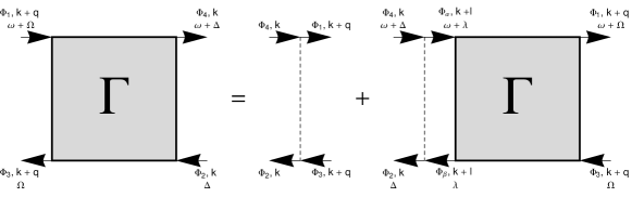
Figure 2: Diagrammatic representation of Bethe-Salpeter equation.

Now, consider $\omega=0$. We separate the summation over eigenstates into two cases: $\Phi_{j}=\Phi_{k}$ and $\Phi_{j}\neq\Phi_{k}$. If $\Phi_{j}=\Phi_{k}$, then $\frac{1}{\beta}\sum_{\lambda}G_{0}\left(\Phi_{j},\lambda\right)^{2}=-\beta\nu_{\Phi_{j}}\left(1-\nu_{\Phi_{j}}\right).$ If $\Phi_{j}\neq\Phi_{k}$, then $\frac{1}{\beta}\sum_{\lambda}G_{0}\left(\Phi_{j},\lambda\right)G_{0}\left(\Phi_{k},\lambda\right)=\frac{\nu_{\Phi_{k}}-\nu_{\Phi_{j}}}{\xi_{\Phi_{k}}-\xi_{\Phi_{j}}}.$ This leads to

$$\Gamma_{\Phi_{\alpha}\Phi_{\beta}\Phi_{\gamma}\Phi_{\delta}}\left(q,0\right) = M_{\Phi_{\alpha}\Phi_{\beta}\Phi_{\gamma}\Phi_{\delta}}\left(0,q\right)+\beta\sum_{\Phi_{j},l}\nu_{\Phi_{j}}\left(1-\nu_{\Phi_{j}}\right)M_{\Phi_{j}\Phi_{\beta}\Phi_{j}\Phi_{\delta}}\left(0,l\right)\Gamma_{\Phi_{\alpha}\Phi_{j}\Phi_{\gamma}\Phi_{j}}\left(q-l,0\right)$$

$$-\sum_{\Phi_{j},\Phi_{k}}\sum_{l}\frac{\nu_{\Phi_{k}}-\nu_{\Phi_{j}}}{\xi_{\Phi_{k}}-\xi_{\Phi_{j}}}M_{\Phi_{k}\Phi_{\beta}\Phi_{j}\Phi_{\delta}}\left(0,l\right)\Gamma_{\Phi_{\alpha}\Phi_{j}\Phi_{\gamma}\Phi_{k}}\left(q-l,0\right).$$ (15)

Equations (LABEL:eq:BetheSalpeterOmegaFinite) and (15) are exact expressions for the two-particle vertex at finite and zero frequency, respectively.

The expressions in Eqs. (LABEL:eq:BetheSalpeterOmegaFinite) and (15) are somewhat cumbersome. Hence, it is instructive to investigate a simpler case than the general situation, in particular, the case where only two states are located near the Fermi energy.

II.1.3 Two states near the Fermi energy

Let $\Phi_{1}$ and $\Phi_{2}$, with energies $\xi_{\Phi_{1}}\leq\xi_{\Phi_{2}}$, label the two states that lie nearest the Fermi surface and assume that both $\nu_{\Phi_{1}}$ and $\nu_{\Phi_{2}}$ are non-zero. We will ignore other states that are either fully occupied or empty. Furthermore, orthogonality of $\Phi_{1}$ and $\Phi_{2}$ leads to the simplification that only four vertices contribute to the one- and two-particle propagators: $M_{\Phi_{1}\Phi_{1}\Phi_{1}\Phi_{1}}\left(0,q\right)$, $M_{\Phi_{2}\Phi_{2}\Phi_{2}\Phi_{2}}\left(0,q\right)$, $M_{\Phi_{1}\Phi_{2}\Phi_{2}\Phi_{1}}\left(0,q\right)$, and $M_{\Phi_{2}\Phi_{1}\Phi_{1}\Phi_{2}}\left(0,q\right)$.

The form of the vertices that are non-vanishing implies that $\mathcal{M}_{\Phi_{\alpha}\Phi_{\beta}}=\mathcal{M}_{\Phi_{\alpha}\Phi_{\alpha}}\delta_{\Phi_{\alpha}\Phi_{\beta}}$, so from Eq. (12) the self-energy of the state $\Phi$ is

$$\Sigma_{\Phi} = -\frac{\nu_{\Phi}\mathcal{M}_{\Phi\Phi}}{1-\beta\nu_{\Phi}\left(1-\nu_{\Phi}\right)\mathcal{M}_{\Phi\Phi}}.$$

Since $\mathcal{M}$ is negative, the self-energy has no poles, and hence is well-behaved for a contact potential.

We can also obtain simple expressions for the two-particle propagator. The condition of orthogonality of $\Phi_{1}$ and $\Phi_{2}$ limits the possible non-zero terms to $\Gamma_{\Phi_{1}\Phi_{1}\Phi_{1}\Phi_{1}}$, $\Gamma_{\Phi_{1}\Phi_{2}\Phi_{2}\Phi_{1}}$, $\Gamma_{\Phi_{2}\Phi_{1}\Phi_{1}\Phi_{2}}$, and $\Gamma_{\Phi_{2}\Phi_{2}\Phi_{2}\Phi_{2}}$. First, consider the case of finite frequency. Taking the Fourier transform of each expression with respect to $q$ with conjugate variable $s$, we can solve for each of the two-particle propagators explicitly. We find that $\tilde{\Gamma}_{\Phi_{1}\Phi_{1}\Phi_{1}\Phi_{1}}\left(s,\omega\right)=\tilde{M}_{\Phi_{1}\Phi_{1}\Phi_{1}\Phi_{1}}\left(0,s\right)$, and $\tilde{\Gamma}_{\Phi_{2}\Phi_{2}\Phi_{2}\Phi_{2}}\left(s,\omega\right)=\tilde{M}_{\Phi_{2}\Phi_{2}\Phi_{2}\Phi_{2}}\left(0,s\right)$ which have no poles, and

$$\tilde{\Gamma}_{\Phi_{1}\Phi_{2}\Phi_{2}\Phi_{1}}\left(s,\omega\right) = \frac{\tilde{M}_{\Phi_{1}\Phi_{2}\Phi_{2}\Phi_{1}}\left(0,s\right)}{1+\tilde{M}_{\Phi_{1}\Phi_{2}\Phi_{2}\Phi_{1}}\left(0,s\right)\frac{\nu_{\Phi_{2}}-\nu_{\Phi_{1}}}{i\omega+\left(\xi_{\Phi_{2}}-\xi_{\Phi_{1}}\right)}},\mathbf{}$$ (16)

$$\tilde{\Gamma}_{\Phi_{2}\Phi_{1}\Phi_{1}\Phi_{2}}\left(s,\omega\right) = \frac{\tilde{M}_{\Phi_{2}\Phi_{1}\Phi_{1}\Phi_{2}}\left(0,s\right)}{1-\tilde{M}_{\Phi_{2}\Phi_{1}\Phi_{1}\Phi_{2}}\left(0,s\right)\frac{\nu_{\Phi_{2}}-\nu_{\Phi_{1}}}{i\omega-\left(\xi_{\Phi_{2}}-\xi_{\Phi_{1}}\right)}}.$$ (17)

The $\tilde{\Gamma}_{\Phi_{1}\Phi_{2}\Phi_{2}\Phi_{1}}\left(s,\omega\right)$ and $\tilde{\Gamma}_{\Phi_{2}\Phi_{1}\Phi_{1}\Phi_{2}}\left(s,\omega\right)$ propagators have poles at finite $\omega$ when $\nu_{\Phi_{1}}\neq\nu_{\Phi_{2}}$. Since there are no poles in the $\mbox{Re}\left(\omega\right)>0$ half-plane, we can analytically continue Matsubara frequencies to real frequencies, $i\omega\to\omega+i\delta$. By symmetry, $\tilde{M}_{\Phi_{1}\Phi_{2}\Phi_{2}\Phi_{1}}\left(0,s\right)=\tilde{M}_{\Phi_{2}\Phi_{1}\Phi_{1}\Phi_{2}}\left(0,s\right)$ so Eqs. (16) and (17) indicate that the system is most susceptible to ordering in states $\Phi_{1}$ and $\Phi_{2}$ at the same wavelength $s_{{\rm CDW}}\left(\omega,T\right)$.

Let $\Delta\nu=\nu_{\Phi_{2}}-\nu_{\Phi_{1}}$ and $\Delta\xi=\xi_{\Phi_{2}}-\xi_{\Phi_{1}}$, and assume $\xi_{\Phi_{2}}>\xi_{\Phi_{1}}$. After analytical continuation, the frequency at which $\Gamma$ diverges is

$$\omega_{c} = \Delta\xi\left[1+\tilde{M}_{\Phi_{1}\Phi_{2}\Phi_{2}\Phi_{1}}\left(0,s\right)\frac{\Delta\nu}{\Delta\xi}\right].$$

At low temperatures, $\omega_{c}\propto$ $\beta$, which implies that $\omega$ diverges as $T\to 0$ unless $\omega\to 0$ at finite temperature. This motivates us to consider the static ($\omega=0$) limit.

In the static limit, all four two-particle vertices are modified by the interaction. The vertices are

$$\tilde{\Gamma}_{\Phi_{1}\Phi_{1}\Phi_{1}\Phi_{1}}\left(s,0\right) = \frac{\tilde{M}_{\Phi_{1}\Phi_{1}\Phi_{1}\Phi_{1}}\left(0,s\right)}{1-\beta\nu_{\Phi_{1}}\left(1-\nu_{\Phi_{1}}\right)\tilde{M}_{\Phi_{1}\Phi_{1}\Phi_{1}\Phi_{1}}\left(0,s\right)},$$ (18)

$$\tilde{\Gamma}_{\Phi_{2}\Phi_{2}\Phi_{2}\Phi_{2}}\left(s,0\right) = \frac{\tilde{M}_{\Phi_{2}\Phi_{2}\Phi_{2}\Phi_{2}}\left(0,s\right)}{1-\beta\nu_{\Phi_{2}}\left(1-\nu_{\Phi_{2}}\right)\tilde{M}_{\Phi_{2}\Phi_{2}\Phi_{2}\Phi_{2}}\left(0,s\right)},$$ (19)

and

$$\tilde{\Gamma}_{\Phi_{1}\Phi_{2}\Phi_{2}\Phi_{1}}\left(s,0\right) = \frac{\tilde{M}_{\Phi_{1}\Phi_{2}\Phi_{2}\Phi_{1}}\left(0,s\right)}{1+\frac{\nu_{\Phi_{2}}-\nu_{\Phi_{1}}}{\xi_{\Phi_{2}}-\xi_{\Phi_{1}}}\tilde{M}_{\Phi_{1}\Phi_{2}\Phi_{2}\Phi_{1}}\left(0,s\right)},$$ (20)

and by symmetry of the interaction vertices, $\tilde{\Gamma}_{\Phi_{1}\Phi_{2}\Phi_{2}\Phi_{1}}\left(s,0\right)=\tilde{\Gamma}_{\Phi_{2}\Phi_{1}\Phi_{1}\Phi_{2}}\left(s,0\right).$ We see in Eqs. (18) and (19) that the system is unstable to CDW formation in $\Phi_{1}$ at a temperature

$$T_{11}=\nu_{\Phi_{1}}\left(1-\nu_{\Phi_{1}}\right)\tilde{M}_{\Phi_{1}\Phi_{1}\Phi_{1}\Phi_{1}}\left(0,s_{1}\right)$$

and in $\Phi_{2}$ at a temperature

$$T_{22}=\nu_{\Phi_{2}}\left(1-\nu_{\Phi_{2}}\right)\tilde{M}_{\Phi_{2}\Phi_{2}\Phi_{2}\Phi_{2}}\left(0,s_{2}\right),$$

where $s_{1}$ and $s_{2}$ maximize $\tilde{M}_{\Phi_{1}\Phi_{1}\Phi_{1}\Phi_{1}}(0,s)$ and $\tilde{M}_{\Phi_{2}\Phi_{2}\Phi_{2}\Phi_{2}}(0,s)$ respectively.

If $\xi_{\Phi_{2}}-\xi_{\Phi_{1}}$ is small, then the filling fractions $\nu_{\Phi_{1}}$ and $\nu_{\Phi_{2}}$ are almost equal. Expanding $\nu_{\Phi_{2}}$ about $\xi_{\Phi_{1}}$ to first order, $\nu_{\Phi_{2}}\approx\nu_{\Phi_{1}}+f^{\prime}\left(\xi_{\Phi_{1}}-\mu\right)\left(\xi_{\Phi_{2}}-\xi_{\Phi_{1}}\right)$. Then $\frac{\nu_{\Phi_{2}}-\nu_{\Phi_{1}}}{\xi_{\Phi_{2}}-\xi_{\Phi_{1}}}\approx-\beta\nu_{\Phi_{1}}\left(1-\nu_{\Phi_{1}}\right)+\mathcal{O}\left(f^{\prime\prime\prime}\left(\xi_{1}\right)\right).$ Eq. (20) allows us to find a third temperature scale, associated with interactions between states 1 and 2:

$$T_{12}=\nu_{\Phi_{1}}\left(1-\nu_{\Phi_{1}}\right)\tilde{M}_{\Phi_{1}\Phi_{2}\Phi_{2}\Phi_{1}}\left(0,s_{12}\right),$$

where $s_{12}$ maximizes $\tilde{M}_{\Phi_{1}\Phi_{2}\Phi_{2}\Phi_{1}}(0,s)$. Whilst we have derived these results for a contact potential, we will see that multiple temperature scales also arise for a Coulomb potential in Sec. IV.

III Landau theory for mixed CDW ordering

There has been considerable work on the Landau theory for interaction induced CDWs in the lowest Landau level,FPA ; Gerhardts and higher Landau levels.KFS ; MoessnerChalker Here we allow for ordering of CDWs of states that arise from Landau level mixing and focus on the situation in which there are two states close to the Fermi energy. We use similar notation to that of Fukuyama et al. (FPA).FPA Furthermore, we modify the notation of previous sections and write $\sum_{\Phi_{i}}\to\sum_{i}$. The analysis in this section leads to a Landau theory where coupling between order parameters of different states becomes important.

III.1 Hartree-Fock Hamiltonian

We consider an interaction $v({\mathbf{q}})$ and start from the interaction Hamiltonian

$$H_{I} = \frac{1}{2}\sum_{\mathbf{q}\neq 0}v\left(\mathbf{q}\right)\left[\hat{\rho}\left(\mathbf{q}\right)\hat{\rho}\left(-\mathbf{q}\right)+\hat{S}_{x}\left(\mathbf{q}\right)\hat{S}_{x}\left(-\mathbf{q}\right)-f\left(\mathbf{q}\right)\right],$$ (21)

which is a natural generalization of the FPA interaction Hamiltonian to a situation with multiple states.Rasolt The operator $\hat{\rho}\left(\mathbf{q}\right)$ is the charge density operator of the two-state system, expressed as

$$\hat{\rho}\left(\mathbf{q}\right) = \sum_{i=1}^{2}\sum_{X}\rho_{iX}\left(\mathbf{q}\right)a_{iX_{+}}^{\dagger}a_{iX_{-}},$$ (22)

where

$$\rho_{iX}\left(\mathbf{q}\right) = \int d^{2}{{\mathbf{r}}}\,e^{-i{\mathbf{q}}\cdot{\mathbf{r}}}\phi^{*}_{iX}({\mathbf{r}})\phi_{iX}({\mathbf{r}})=e^{-iq_{x}X}A_{ii}(\mathbf{q}),$$ (23)

where $\phi_{iX}({\mathbf{r}})=\sum_{\alpha}C_{i\alpha}\psi_{X}^{(n_{\alpha})}({\mathbf{r}})$, with $\psi$ defined in Eq. (1), and with

$$A_{ij}\left(\mathbf{q}\right) = \sum_{\alpha}\sqrt{\frac{n_{ij_{\alpha}}^{\prime}!}{\left(n_{ij_{\alpha}}^{\prime}+\delta n_{ij_{\alpha}}\right)!}}C^{*}_{i\alpha}C_{j\alpha}e^{-i\left(n_{i_{\alpha}}-n_{j_{\alpha}}\right)\left(\theta-\pi/2\right)}e^{-\frac{\left(ql_{0}\right)^{2}}{4}}\left[\frac{(ql_{0})^{2}}{2}\right]^{\delta n_{ij}/2}\mathcal{L}^{\delta n_{ij_{\alpha}}}_{n_{ij_{\alpha}}^{\prime}}\left[\frac{\left(ql_{0}\right)^{2}}{2}\right],$$ (24)

where $n_{ij_{\alpha}}^{\prime}=\min\left(n_{i_{\alpha}},n_{j_{\alpha}}\right)$, $\delta n_{ij_{\alpha}}=\left|n_{i_{\alpha}}-n_{j_{\alpha}}\right|$, and $\theta=\arctan\left(q_{y}/q_{x}\right)$. The operator $S_{x}\left(\mathbf{q}\right)$ is a pseudospin density operator

$$\hat{S}_{x}\left(\mathbf{q}\right) = \sum_{i,j=1}^{2}\sum_{X}s_{ij,X}\left(\mathbf{q}\right)a_{iX_{+}}^{\dagger}a_{jX_{-}},$$ (25)

where

$$s_{ij,X}\left(\mathbf{q}\right) = \sigma_{x}^{ij}\int d^{2}{\mathbf{r}}\,e^{-i{\mathbf{q}}\cdot{\mathbf{r}}}\phi_{jX}^{*}({\mathbf{r}})\phi_{iX}({\mathbf{r}})=\sigma_{x}^{ij}e^{-iq_{x}X}A_{ij}(\mathbf{q}),$$ (26)

and $\sigma_{x}$ is the Pauli matrix. The first term in $H_{I}$ describes interactions between fermions in the same eigenstate, while the second term describes interactions between fermions in differing eigenstates. Such a term can generically be expected to be present in the situation we consider here,Rasolt but usually will have a smaller magnitude than the first term in $H_{I}$ (which is the case here). The final term in $H_{I}$ is

$$f\left(\mathbf{q}\right) = \sum_{i=1}^{2}A_{ii}\left(\mathbf{q}\right)^{2}\rho_{i}(0).$$ (27)

We use different notation from the notation in Sec. II by labeling states with $X=kl_{0}^{2}$ rather than pseudomomentum $k$, and $X_{\pm}=X\pm\frac{1}{2}q_{y}l_{0}^{2}$. The indices $i$ and $j$ take values of 1 or 2 and label states $\Phi_{i}$ and $\Phi_{j}$. The operators $a^{\dagger}_{iX_{\pm}}$ ($a_{iX_{\pm}}$) create (annihilate) a fermion in the non-interacting eigenstate $\Phi_{i}$ with guiding centre coordinate $X_{\pm}=X\pm\frac{q_{y}l_{0}^{2}}{2}$, and satisfy the usual anticommutation relations $\left\{a_{iX_{\pm}},a^{\dagger}_{jY_{\pm}}\right\}=\delta_{ij}\delta_{X_{\pm},Y_{\pm}}$. In the limit of no mixing, and when restricted to the lowest LL, the interaction Hamiltonian reduces to the form considered by FPA.

The total number of fermions in the two-state system is $N=N_{1}+N_{2}=\frac{L^{2}}{2\pi l_{0}^{2}}$, where

$$N_{i} = \left<\sum_{X}a_{iX}^{\dagger}a_{iX}\right>,$$ (28)

is the number of electrons in state $\Phi_{i}$. Similarly to FPA, we define the order parameter for a CDW in eigenstate $\Phi_{i}$, $\Delta_{i}\left(\mathbf{Q}_{i}\right)$ by

$$\left\langle a_{iX_{+}}^{\dagger}a_{jX_{-}}\right\rangle = \frac{2\pi}{L}\delta_{ij}P_{i}\sum_{\mathbf{Q}_{i}}\left[\Delta_{i}^{*}\left(\mathbf{Q}_{i}\right)e^{i\left(Q_{i}\right)_{x}X}\delta\left(\left(Q_{i}\right)_{y}-q_{y}\right)+\Delta_{i}\left(\mathbf{Q}_{i}\right)e^{-i\left(Q_{i}\right)_{x}X}\delta\left(\left(Q_{i}\right)_{y}+q_{y}\right)\right],$$ (29)

where $P_{i}=N_{i}/N$ is the fraction of the fermions that occupy state $\Phi_{i}$. Each order parameter depends on a unique set of wavevectors $\left\{\mathbf{Q}_{i}\right\}$, where $\mathbf{Q}_{i}=\left(\left(Q_{i}\right)_{x},\left(Q_{i}\right)_{y}\right)$. The summation over wavevectors allows for CDW ordering at several wavevectors. For instance, a triangular CDW can be described by a set of three wavevectors of equal length, oriented at angles $\frac{2\pi}{3}$ with respect to each other,FPA whereas a striped CDW is described by a single wavevector.MoessnerChalker Furthermore, note that the order parameters are defined such that $\Delta_{i}^{*}\left(\mathbf{Q}_{i}\right)=\Delta_{i}\left(-\mathbf{Q}_{i}\right)$, which follows from Eq. (29).

Next, we use the Hartree-Fock approximation to rewrite the Hamiltonian as:

$$H = H_{0}+H_{{\rm CDW}}+N\sum_{i=1}^{2}\sum_{\left\{\mathbf{Q}_{i}\right\}}P_{i}^{2}U_{ii}\left(Q_{i}\right)|\Delta(Q_{i})|^{2},$$

where

$$H_{0}=\sum_{i=1}^{2}\sum_{X}\epsilon_{i}^{0}a_{iX}^{\dagger}a_{iX},$$

is the non-interacting Hamiltonian with $\epsilon_{i}^{0}$ the energy of single particle eigenstate $\Phi_{i}$, and

$$H_{\rm CDW} = -\left\{\sum_{i=1}^{2}\sum_{\left[\mathbf{Q}_{i}\right\}}P_{i}U_{ii}\left(Q_{i}\right)\sum_{X}\left[\Delta_{i}\left(\mathbf{\mathbf{Q}_{i}}\right)e^{i(Q_{i})_{x}X}a_{iX_{-}}^{\dagger}a_{iX_{+}}+\Delta_{i}^{*}\left(\mathbf{\mathbf{Q}_{i}}\right)e^{-i(Q_{i})_{x}X}a_{iX_{+}}^{\dagger}a_{iX_{-}}\right]\right.$$

$$\left.+\sum_{i=1}^{2}\sum_{j\neq i}P_{i}U_{ij}\left(Q_{i}\right)\sum_{X}\left[\Delta_{i}\left(\mathbf{Q}_{i}\right)e^{i(Q_{i})_{x}X}a_{jX_{-}}^{\dagger}a_{jX_{+}}+\Delta_{i}^{*}\left(\mathbf{Q}_{i}\right)e^{-i(Q_{i})_{x}X}a_{jX_{+}}^{\dagger}a_{jX_{-}}\right]\right\}.$$

We let $Q_{i}=\left|\mathbf{Q}_{i}\right|$ and $\theta_{i}=\arctan\left[\frac{\left(Q_{i}\right)_{y}}{\left(Q_{i}\right)_{x}}\right]$ and henceforth we absorb $l_{0}$ in the definition of $q$, i.e. $ql_{0}\to q$. In the summations over wavevectors, we sum over $\left\{\mathbf{Q}_{i}^{\alpha}\right\}_{\alpha=1}^{n}$, where $n$ is the number of wavevectors describing the CDW state. Furthermore, we define the following functions, which describe the Hartree-Fock interaction potentials:

$$U_{ii}\left(Q_{i}\right) = \int\mbox{d}q\hskip 1.42271ptq\hskip 1.42271ptv\left(q\right)A_{ii}\left(q\right)^{2}J_{0}\left(qQ_{i}\right)-v\left(Q_{i}\right)A_{i}\left(Q_{i}\right)^{2},$$

$$U_{ij}\left(Q_{i}\right) = \frac{1}{2\pi}\sum_{m=-\infty}^{\infty}\int\mbox{d}^{2}\mathbf{q}\hskip 1.42271ptv\left(q\right)A_{ij}\left(q\right)A_{ji}\left(q\right)J_{m}\left(qQ_{i}\right)-v\left(Q_{i}\right)A_{i}\left(Q_{i}\right)A_{j}\left(Q_{i}\right),$$

The potentials $U_{ii}$ and $U_{ij}$ represent the most significant contributions to the Hartree-Fock Hamiltonian. We ignore other terms generated by the Hartree-Fock approximation, as their contributions are negligible.

III.2 Landau theory

We construct a Landau theory in the spirit of FPA by considering the difference in free energy between a uniform system and an ordered system for a fixed total number of electrons, $N$. We write the difference in free energy, $\delta F$, in terms of the grand potentials of each system,

$$\delta F=\Omega_{\rm CDW}\left(\mu\right)-\Omega_{0}\left(\mu\right)+\frac{1}{2}\left(\mu-\mu_{0}\right)^{2}\frac{\partial^{2}\Omega_{0}\left(\mu_{0}\right)}{\partial\mu_{0}^{2}},$$

where $\Omega_{\rm CDW}$ and $\Omega_{0}$ are the grand potentials of the CDW and uniform systems, respectively, and the chemical potentials of the uniform and CDW systems are $\mu_{0}$ and $\mu$, respectively, and we expand in powers of the CDW order parameters $\Delta_{1}\left(\mathbf{Q}_{1}\right)$ and $\Delta_{2}\left(\mathbf{Q}_{2}\right)$.

The grand potential when there is CDW ordering is

$$\Omega_{\rm CDW}\left(\mu\right) = -\beta^{-1}\ln\left\{\mbox{Tr}\left[e^{-\beta\left(H-\mu\sum_{i}\sum_{X}\hat{n}_{iX}\right)}\right]\right\}$$

$$= \Omega_{0}\left(\mu\right)-\beta^{-1}\ln\left\langle e^{-\beta H_{\rm CDW}}\right\rangle_{0}+N\sum_{i=1}^{2}\sum_{\left\{\mathbf{Q}_{i}\right\}}P_{i}^{2}U_{ii}\left(Q_{i}\right)\left|\Delta_{i}\left(\mathbf{Q}_{i}\right)\right|^{2},$$

where $\left<\ldots\right>_{0}$ indicates an average with respect to the uniform state, $H_{{\rm CDW}}$ is defined above in Eq. (LABEL:eq:HamiltonianHartreeFock), and

$$\Omega_{0}\left(\mu\right) = -N\beta^{-1}\sum_{i}\ln\left[1+e^{-\beta\left(\epsilon_{i}^{0}-\mu\right)}\right].$$

We now develop the perturbative expansion of the free energy in terms of the order parameters $\Delta_{1}\left(\mathbf{Q}_{1}\right)$ and $\Delta_{2}\left(\mathbf{Q}_{2}\right)$. We expand the logarithm, which gives

$$\frac{\delta F}{N} = \sum_{i=1}^{2}\sum_{\left\{\mathbf{Q}_{i}\right\}}P_{i}^{2}U_{ii}\left(Q_{i}\right)\left|\Delta_{i}\left(\mathbf{Q}_{i}\right)\right|^{2}-\frac{1}{N}\sum_{p=1}^{\infty}\frac{\left(-1\right)^{p}\beta^{p-1}}{p!}\left\langle\left(H_{\rm HF}\right)^{p}\right\rangle_{0}+\frac{1}{2N}\left(\mu-\mu_{0}\right)^{2}\frac{\partial^{2}\Omega_{0}\left(\mu_{0}\right)}{\partial\mu_{0}^{2}}.$$ (32)

The $p=1$ term in the expansion vanishes, since it involves averages of the form $\left\langle a_{iX_{+}}^{\dagger}a_{iX_{-}}\right\rangle_{0}=\delta_{X_{+}X_{-}}$ which imply $\mathbf{Q}_{i}=0$. We consider Eq. (32) to fourth order in both order parameters and write the CDW order parameters in the form $\Delta_{k}=\Delta_{k}\left(\mathbf{Q}_{k}\right)$. The general form of the free energy density when ${\mathbf{Q}}_{1}\neq{\mathbf{Q}}_{2}$ is

$$\mathcal{F} = P_{1}^{2}a_{1}\left(\mathbf{Q}_{1},T\right)|\Delta_{1}|^{2}+P_{2}^{2}a_{2}\left(\mathbf{Q}_{2},T\right)|\Delta_{2}|^{2}+P_{1}^{3}b_{1}\left(\mathbf{Q}_{1},T\right)|\Delta_{1}|^{3}+P_{2}^{3}b_{2}\left(\mathbf{Q}_{1},T\right)|\Delta_{2}|^{3}$$ (33)

$$\hskip 2.84544pt+P_{1}^{4}c_{1}\left(\mathbf{Q}_{1},T\right)|\Delta_{1}|^{4}+P_{2}^{4}c_{2}\left(\mathbf{Q}_{2},T\right)|\Delta_{2}|^{4}+P_{1}^{2}P_{2}^{2}\gamma\left(\mathbf{Q}_{1},\mathbf{Q}_{2},\theta,T\right)|\Delta_{1}|^{2}|\Delta_{2}|^{2},$$

where $\mathcal{F}=\delta F/N$. We calculate the coefficients $a_{i}$, $b_{i}$, $c_{i}$ and $\gamma$ explicitly within the Hartree-Fock approximation allowing for the possibility of either striped or triangular CDW order in either state 1 or state 2. The striped phase is described by a single wavevector while the triangular CDW is described by a set of three wavevectors of equal magnitude, oriented at 120^∘ with respect to each other. The expressions for these coefficients are quite lengthy and we present them in full detail in Appendix A. The phase behaviour of free energies of the form in Eq. (33) when $b_{1}=b_{2}=0$ was studied in detail by Imry.Imry In general, there are three possible critical points, with free energies $\mathcal{F}_{1}$, $\mathcal{F}_{2}$, and $\mathcal{F}_{M}$. If $\mathcal{F}_{1}$ is globally minimum, then $\Delta_{1}\neq 0$, and $\Delta_{2}=0$ and vice versa for $\mathcal{F}_{2}$. If $\mathcal{F}_{M}$ is the global minimum, then both $\Delta_{1}\neq 0$ and $\Delta_{2}\neq 0$. In the case we consider, the phases associated with $\mathcal{F}_{1}$ and $\mathcal{F}_{2}$ are CDW ground states in either state $\Phi_{1}$ or $\Phi_{2}$, respectively. The phases associated with $\mathcal{F}_{M}$ are mixed CDW states. The mixed CDW phase exists only when the parameter $\gamma$, which couples ordering in states 1 and 2 is finite. If $\gamma>0$, then there is competition between order parameters of each state; if $\gamma<0$, then ordering in one state serves to enhance ordering in the other.Imry The phases of the order parameters are important only for triangular CDWs.FPA If the phases corresponding to the three different order parameters are denoted by $\left\{\phi_{i}\right\}_{i=1}^{3}$, then for a state $\Phi$, $\phi_{1}+\phi_{2}+\phi_{3}=0\mbox{ }(\pi)$ if $\nu_{\Phi}<1/2$ $(>1/2)$.

There are additional terms in the free energy that are allowed when ${\mathbf{Q}}_{1}={\mathbf{Q}}_{2}$, which take the form

$$\delta{\mathcal{F}}_{{\mathbf{Q}}_{1}={\mathbf{Q}}_{2}} = P_{1}P_{2}\alpha\left|\Delta_{1}\right|\left|\Delta_{2}\right|+P_{1}^{2}P_{2}\eta\left|\Delta_{1}\right|^{2}\left|\Delta_{2}\right|+P_{1}P_{2}^{2}\varphi\left|\Delta_{1}\right|\left|\Delta_{2}\right|^{2}+P_{1}^{2}P_{2}^{2}\tilde{\gamma}\left|\Delta_{1}\right|^{2}\left|\Delta_{2}\right|^{2}$$ (34)

$$\hskip 2.84544pt+P_{1}^{3}P_{2}\sigma\left|\Delta_{1}\right|^{3}\left|\Delta_{2}\right|+P_{1}P_{2}^{3}\rho\left|\Delta_{1}\right|\left|\Delta_{2}\right|^{3}.$$

The coefficients $\alpha$, $\eta$, $\varphi$, $\tilde{\gamma}$, $\sigma$, and $\rho$ depend on the magnitude of the ordering wavevectors $Q_{1}=Q_{2}=Q$ and the relative phases of the order parameters. Note that $\tilde{\gamma}$ modifies $\gamma\left(\mathbf{Q},\mathbf{Q},0,T\right)$ in the case of equal wavevectors. These coefficients are displayed in Appendix B.

We adopt the following notation for describing the possible phases. For ordering in a single state, we label according to the symmetry and state index. For example, striped (triangular) ordering in $\Phi_{1}$ is denoted S1 (T1). For mixed CDW ordering, we label according to the symmetry of the order parameter for each phase with order in $\Phi_{1}$ preceding that in $\Phi_{2}$. For example, mixed CDW ordering between striped phases in both states is labeled SS. If the wavevectors for each phase are equal, we add an extra “E” to the end of the label. In all, we allow for the possibility of 12 types of CDW ordering: S1, S2, T1, T2, SS, TT, ST, TS, SSE, TTE, STE, and TSE. We present results for specific numerical examples in Sec. IV.

IV Numerics

The Landau theory developed in Sec. III makes no assumptions about the source of LL mixing, and does not specify the interaction $v({\mathbf{q}})$. There are many possible sources of LL mixing in 2DEGs that can affect CDW order, such as electron-electron interactionsMacDonald or disorder.Stanescu However, we focus on the specific example of Rashba spin-orbit coupling, since this may give a way to tune levels into degeneracy controllably and create a situation of the form discussed in Sec. III. Electron-electron interactions are described by an unscreened Coulomb potential – we expect that screening may lead to small quantitative changes in our results, but that our qualitative results will be robust as we discuss in Sec. IV.1.2

IV.1 Model and parameters

IV.1.1 Rashba spin-orbit coupling

Rashba spin orbit coupling can be significant in GaAs quantum wells and leads to LL mixing. For holes near the $\Gamma$ point in GaAs there are four $j=3/2$ spin states in the valence band, which separate into two heavy-hole (HH) and two light-hole (LH) states with different effective masses. The heavy hole states correspond to angular momentum $j_{z}=\pm 3/2$ and the light hole states correspond to $j_{z}=\pm 1/2$. The strength of Rashba coupling can be tuned through external means, such as a back gate, which allows tuning of levels into and out of degeneracy. Generically, Dresselhaus spin-orbit coupling will also be present in GaAs, however, we focus on the regime where Rashba coupling is dominant and ignore additional (non-tunable) mixing that may arise from Dresselhaus coupling.

We specify the single-particle Hamiltonian, which includes Rashba coupling and Zeeman splitting, as

$$H_{\rm non-interacting} = H_{0}+H_{z}+H_{SO},$$ (35)

and diagonalize to find the non-interacting eigenstates as a function of the strength of the magnetic field and the Rashba coupling. We then consider a specific example in which there are two energy levels that are close to degeneracy at a particular value of Rashba coupling, and explore the effects of interactions on the phase diagram as a function of temperature, filling and Rashba coupling.

We take the free-particle Hamiltonian to be

$$H_{0}=\sum_{j_{z}}\hbar\omega(|j_{z}|)\left(\hat{n}_{j_{z}}+\frac{1}{2}\right),$$

where

$$\omega(|j_{z}|)=\left\{\begin{array}[]{ccc}\omega_{HH}&{\rm for}&j_{z}=\pm\frac{3}{2}\\ \\ \omega_{LH}&{\rm for}&j_{z}=\pm\frac{1}{2}\end{array}\right.,$$

and the number operator $\hat{n}_{j_{z}}=a^{\dagger}_{j_{z}}a_{j_{z}}$, with $a^{\dagger}_{j_{z}}$ the LL raising operator for a hole with $J_{z}$ eigenvalue $j_{z}$. $\omega_{HH}$ and $\omega_{LH}$ are the cyclotron frequencies of the heavy and light hole states, respectively. The Zeeman splitting term is given by

$$H_{Z} = -g^{*}\mu_{B}B\hat{J}_{z},$$

where the effective $g$-factor for the holes is $g^{*}$. The third operator may be written as

$$H_{SO} = -\alpha\mathcal{R}_{8v8v}\left\langle\mathcal{E}_{z}^{0}\right\rangle\left({\mathbf{k}}\times{\mathbf{J}}\right)_{z},$$

which introduces Rashba spin-orbit coupling into the Hamiltonian. The parameter $\mathcal{R}_{8v8v}$ is a material-dependent Rashba coefficient; $\left\langle\mathcal{E}_{z}^{0}\right\rangle=\frac{e}{2\epsilon}\rho$ is the electric field due to the fermions in the absence of a substrate field.WinklerBook We use parameters that are closely related to those relevant to Fischer et al.’s experiments. We choose material parameters $g^{*}=1.2$, $\mathcal{R}_{8v8v}=14.62\,e{\rm\AA}^{2}$, and $\epsilon=12.4\,\epsilon_{0}$, appropriate to bulk GaAs;WinklerBook we set the heavy- and light-hole masses equal to $m_{H}=0.51m_{0}$ and $m_{L}=0.08m_{0}$, respectively;GaAsParameters and we set the in-plane carrier density to $\rho=3.5\times 10^{11}$ cm^-2.Schmult

We model the effect of tuning via external means (such as a back gate) by the parameter $\alpha$. The magnetic field $B$ is fixed according to the total filling fraction of the system, $\nu_{T}=2\pi\rho l_{0}^{2}$. The term $\alpha\left\langle\mathcal{E}_{z}^{0}\right\rangle$ may be compared to the average confinement electric field seen by fermions in a triangular potential, as discussed by Fischer et al.Grayson The parameter $\alpha$ then corresponds to the enhancement of the average electric field by increasing the substrate electric field, $\mathcal{E}_{s}$. That is, $\alpha=1+\frac{\mathcal{E}_{s}}{\left\langle\mathcal{E}_{z}^{0}\right\rangle}.$ For no substrate field, $\alpha=1$, whereas in the Fischer et al. experiments, $\alpha\approx$ 2-3 corresponding to nonzero $\mathcal{E}_{s}$. For the levels we study here, a crossing takes place for $\alpha_{0}\simeq 20$. The values of $\alpha$ at which level crossings occur are very sensitive to the model parameters. In particular, the values of the material parameters, such as the effective masses and the carrier density, and the presence or absence of Dresselhaus coupling can alter the positions of crossings and the nature of the levels that cross dramatically. Fischer et al. construct a Hamiltonian from the $\Gamma_{6}^{c}$, $\Gamma_{8}^{v}$, and $\Gamma_{7}^{v}$ bands, whereas we consider the $\Gamma_{8}^{v}$ band only. Second, they include both the Rashba and Dresselhaus spin-orbit coupling terms, whereas we consider Rashba coupling only. Third, we set the carrier density to the upper limit studied by Schmult et al.,Schmult which is larger than any of the densities studied by Grayson et al. This choice of carrier density increases the energy gap between the energy levels comprising the two-state system and the nearby energy levels, as shown in Fig. (3), thereby allowing us to focus on states $\Phi_{1}$ and $\Phi_{2}$ only. Whilst our numerical calculations are not adequate for a quantitative discussion of the experiments in Ref. Grayson, , the crossings we are able to induce with increasing $\alpha$ in our simplified model should lead to a qualitative understanding of the effect of LL mixing on CDW formation. As we point out in Sec. IV.3.3 there are certain features in the phase diagram we expect to be generic and others that may depend more sensitively on details of LL mixing.

We diagonalize the Hamiltonian shown in Eq. (35) and find the eigenvectors and associated eigenvalues as functions of $\alpha$ and magnetic field. The non-linear dependence of the energy levels on magnetic field allows for energy crossings.WinklerBook Cubic and tetrahedral corrections can modify these crossings to anti-crossings.Grayson Motivated by the results of Fischer et al.Grayson we focus on parameter values at which there are two energies that are close to degenerate and located near the Fermi energy. This is the situation we discussed in Sec. III. In the vicinity of such a crossing, we write the filling fraction $\nu=\bar{\nu}+\nu_{0}$, where $\bar{\nu}$ is an integer, corresponding to the number of fully occupied energy levels, and $\nu_{0}=\nu_{1}+\nu_{2}$ is the total filling fraction of the two partially filled energy levels. We label the crossing states $\Phi_{1}$ and $\Phi_{2}$, their associated energies $E_{1}$ and $E_{2}$, and their filling fractions $\nu_{1}$ and $\nu_{2}$. Our analysis is not greatly affected if crossings are replaced by anti-crossings, as the key point is that there be non-zero filling in the two states, which will be the case when the temperature is not too low for an anti-crossing. As $T\to 0$, only the lowest energy state is occupied, which decouples the two states, except when $E_{1}=E_{2}$.

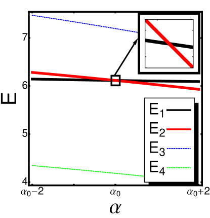
Figure 3: Plot of energy of non-interacting eigenstates $\Phi_{1}$ and $\Phi_{2}$ versus tuning parameter $\alpha$ at $\nu_{T}=7.5$. Energy is in units of $E_{0}=\hbar eB/m_{0}$ and $\alpha$ is dimensionless. The nearest energy levels above and below $E_{1}$ and $E_{2}$ are labeled $E_{4}$ and $E_{3}$, respectively. Inset: Energy levels $E_{1}$ and $E_{2}$ for $\alpha\in[\alpha_{0}-0.01,\alpha_{0}+0.01]$.

IV.1.2 Interactions

We choose the interactions between holes to be given by the unscreened Coulomb interaction, similarly to FPAFPA

$$v\left(\mathbf{q}\right)=\frac{2\pi}{A}\frac{e^{2}}{4\pi\epsilon\left|\mathbf{q}\right|},$$

where $A$ is the area of the 2DHS (the factor $2\pi/A$ comes from the Fourier transform of the real-space Coulomb potential). This allows for a somewhat more realistic interaction than the contact potential considered in Sec. II.

When there are multiple filled Landau levels, the filled levels can act as a background that screens the bare Coulomb interaction. It was found by Aleiner and GlazmanAleinerGlazman (AG) that the screening from filled Landau levels can be accounted for by replacing $\epsilon$ with

$$\epsilon_{AG}\left(q\right) = \left\{1+\frac{2}{qa_{B}}\left[1-J_{0}\left(qR_{L}\right)^{2}\right]\right\}\epsilon_{0},$$ (36)

where $R_{L}=v_{F}/\omega_{c}$ and $a_{B}$ are the Larmor radius and Bohr radius, respectively. Fogler, Koulakov and ShklovskiiFKS used this screened interaction to show that electrons in a partially filled LL near half-filling preferentially order in a striped CDW phase in a weak magnetic field. Away from half-filling, they found ordering in a triangular CDW phase.FKS

In the $n^{\rm th}$ LL at wavevectors $ql_{0}\approx 1/\sqrt{n}$, $\epsilon_{AG}\approx R_{L}/a_{B}$; at low magnetic fields, $\epsilon_{AG}$ is large and screening effects are appreciable. However, at wavevectors $ql_{0}\gtrsim 1$ or $ql_{0}\lesssim 1/n$, screening is negligible. In the example considered in this paper, the CDW ordering generally occurs when $ql_{0}\gtrsim 1$ for an unscreened Coulomb interaction. This is outside the region where the effects of screening would be seen clearly if we considered the modified dielectric constant in Eq. (36). For the purpose of this work, we consider the bare Coulomb interaction as we focus on non-interacting states for which the dominant constituent LLs have $n\leq 4$, hence we expect our phase diagrams to be qualitatively correct, although screening may lead to small quantitative corrections.

IV.1.3 States

Our approach to finding phase diagrams numerically starts by identifying a pair of states which have a crossing. In Fig. 3, we plot the energy of states that we label $\Phi_{1}$ and $\Phi_{2}$ for a magnetic field $B$ corresponding to $\nu_{T}=8$ for our chosen electron density. In addition to these states, we also plot the nearest energy levels above and below $\Phi_{1}$ and $\Phi_{2}$. At $B\approx 1.8$ T the minimum energy gap to the levels above and below $\Phi_{1}$ and $\Phi_{2}$ is approximately 0.23 meV $\sim 2.7$ K, which is large compared to the spacing between $\Phi_{1}$ and $\Phi_{2}$, which is approximately 2.3 $\mu$eV. In comparison, the transition temperature we calculate for the CDW phase is $\sim 10$ K. The Hartree-Fock approximation thus overestimates the transition temperatures observed in experiment, in which anisotropic transport develops for $T\lesssim 100$ mK.Dorsey1 Nevertheless, we ignore adjacent energy levels and construct a two-state system from the crossing energy levels, and make only qualitative predictions about the possibility of CDW ordering as a function of $\nu_{T}$ and $\alpha$. In the situation shown in Fig. 3 there are seven filled levels, and we investigate CDW ordering in the two states near the Fermi energy for $0.5\leq\nu_{0}\leq 1$.

IV.2 Quantum Hall Ferromagnetism

We have focused primarily on the possibility of CDW ordering when two energy levels are in the vicinity of the Fermi energy, and each level has nonzero filling. When two levels are degenerate or close to degenerate then the physics of quantum Hall pseudospin ferromagnetism can also be important.MPB ; JungwirthMacdonald Following Jungwirth and Macdonald,JungwirthMacdonald we determine the Landau theory for quantum Hall pseudospin ferromagnetism when there is Landau level mixing using the Hartree-Fock approximation. This allows us to compare the ordering temperature for quantum Hall ferromagnetism with the temperature we have determined for CDW formation in the vicinity of degeneracy for the non-interacting states.

We define the psuedospin operators in terms of the creation and annihilation operators of the non-interacting eigenstates:

$$\hat{m}_{I,\mathbf{q}} = \sum_{X}a^{\dagger}_{iX_{+}}\sigma_{I}^{(ij)}a_{jX_{-}}e^{-iq_{x}X},$$ (37)

where $\sigma_{I}$ is the Pauli spin matrix and $I=0$, $x$, $y$, and $z$ are pseudospin labels ($\sigma_{0}$ is the two-dimensional identity operator). By construction, $\hat{m}^{\dagger}_{I,q_{y}}=\hat{m}_{I,-q_{y}}$. We focus on ${\mathbf{q}}=0$ order, so the order parameter is defined as

$$m_{I} = \frac{2\pi}{L}\delta_{\mathbf{q},0}\left<a^{\dagger}_{iX_{+}}\sigma_{I}^{(ij)}a_{jX_{-}}\right>.$$ (38)

Since the total filling fraction of the two-state system is fixed, $m_{0}=\nu_{T}$.

We rewrite the creation and annihilation operators of states $\Phi_{1}$ and $\Phi_{2}$ in terms of the pseudospin operators and proceed using the Hartree-Fock approximation in the same manner as outlined in Sec. III or Ref. JungwirthMacdonald, . This leads to the effective Hamiltonian

$$H_{QHF} = \sum_{I=0,z}b_{I}m_{I}-\sum_{IJ=0,x,y,z}W_{IJ}m_{I}\hat{m}_{J,0}+\frac{N}{2}\sum_{IJ=0,x,y,z}W_{IJ}m_{I}m_{J},$$ (39)

where $b_{0}=\frac{\epsilon_{1}^{0}+\epsilon_{2}^{0}}{2}-\frac{1}{2}\sum_{I}W_{II}$ and $b_{z}=\frac{\epsilon_{1}^{0}-\epsilon_{2}^{0}}{2}-W_{0z}$. The potentials $W_{IJ}$ are defined explicitly in Appendix C. We note that for the eigenstates relevant to the numerical example shown below, $W_{0I}=W_{zI}=0$, $I=x,$ $y$, and so $m_{0}$ and $m_{z}$ do not couple to $m_{x}$ and $m_{y}$.

To second order in the pseudospin order parameters, the change in free energy associated with ordering in a QHF takes the form:

$$\delta f_{QHF} = \sum_{I=0,z}b_{I}m_{I}+\sum_{IJ=0,z}W_{IJ}m_{I}\left<\hat{m}_{J,0}\right>_{0}$$ (40)

$$+\frac{1}{2}\sum_{IJ}W_{IJ}m_{I}m_{J}-\frac{\beta}{2}\sum_{IK,JL}W_{IK}W_{JL}m_{I}m_{J}\left<\hat{m}_{K,0}\hat{m}_{L,0}\right>_{0}.$$

The $\left<...\right>_{0}$ notation indicates that we average over non-interacting states. Thus, $\left<\hat{m}_{0,0}\right>_{0}=\nu_{1}+\nu_{2}=\nu_{T}$ and $\left<\hat{m}_{z,0}\right>_{0}=\nu_{1}-\nu_{2}=\delta\nu$. It follows that

$$\delta f_{QHF} = \frac{1}{2}W_{00}m_{0}^{2}\left[1+\left(f^{\prime}_{1}+f^{\prime}_{2}\right)\left(W_{00}+\frac{W_{z0}^{2}}{W_{00}}\right)+\left(f^{\prime}_{1}-f^{\prime}_{2}\right)W_{0z}\right]$$ (41)

$$+\frac{1}{2}W_{xx}m_{x}^{2}\left[1-\beta\left(\nu_{T}-2\nu_{1}\nu_{2}\right)W_{xx}\right]$$

$$+\frac{1}{2}W_{yy}m_{y}^{2}\left[1-\beta\left(\nu_{T}-2\nu_{1}\nu_{2}\right)W_{yy}\right]$$

$$+\frac{1}{2}W_{zz}m_{z}^{2}\left[1+\left(f^{\prime}_{1}+f^{\prime}_{2}\right)\left(W_{zz}+\frac{W_{z0}^{2}}{W_{zz}}\right)+\left(f^{\prime}_{1}-f^{\prime}_{2}\right)W_{0z}\right]$$

$$+\left[\nu_{T}W_{00}+\delta\nu W_{0z}-b_{0}\right]m_{0}+\left[\nu_{T}W_{0z}+\delta\nu W_{zz}+b_{z}\right]m_{z}$$

$$+\left[W_{0z}\left(f^{\prime}_{1}+f^{\prime}_{2}\right)\left(W_{00}+U_{zz}\right)+\left(f^{\prime}_{1}-f^{\prime}_{2}\right)\left(W_{00}U_{zz}+W_{0z}^{2}\right)\right]m_{0}m_{z}.$$

Since $m_{0}$ is constant, $\partial\delta f_{QHF}/\partial m_{0}=0$. Thus, terms containing $m_{0}$ only act to shift the minimum of the free energy, and can be ignored safely. Let us then write the remaining terms as follows:

$$\delta f_{QHF} = \frac{1}{2}\sum_{I=x,y,z}a_{I}\left(T\right)W_{II}m_{I}^{2}+\tilde{b}_{z}\left(T\right)m_{z}.$$

The coefficients $a_{I}$ determine the temperature scales for a second-order phase transition into a quantum Hall ferromagnetic state, whilst the coefficient $\tilde{b}_{z}$ acts as a symmetry-breaking field. We include the transition temperatures $T_{QHF}$ obtained from the condition $a_{I}=0$ in the numerical examples in Sec. IV.3 below.

IV.3 Phase Diagrams

We study the phase diagram as a function of $\alpha$, $\nu_{T}$ and $T$ in two different directions in parameter space. First we vary $\nu_{T}$ from 7.5 to 8.0 when the energy levels are degenerate. Second, we vary $\alpha$ at fixed $\nu_{T}=7.5$ and 8.0. It should be notedMoessnerChalker that the free energy expansion is strictly only valid when the order parameters are small and is hence most applicable near the transition temperature into an ordered state. Thus, at a given $\alpha$ and $\nu_{T}$, we consider the ground state to be the state with the highest ordering temperature.

IV.3.1 Degenerate energy levels

In Fig. 4 we show the phase diagram as a function of $\nu_{T}$ for the energy levels found in Sec. IV.1.3 when the two states are degenerate. As shown in the inset, when $\nu_{T}\simeq 8.0$, there is a transition from the uniform phase to the SSE phase. As $\nu_{T}$ is decreased from 8.0, the transition from uniform to CDW ordering prefers the TTE phase. Below the transition temperature, the transition between the SSE and TTE phases is first-order, and is a function of temperature and total filling fraction. Note that the Quantum Hall ferromagnetism temperature $T_{QHF}$ is lower than the CDW ordering temperature for all $\nu_{T}$ considered. Thermal and quantum fluctuations might change this ordering of transition temperatures.

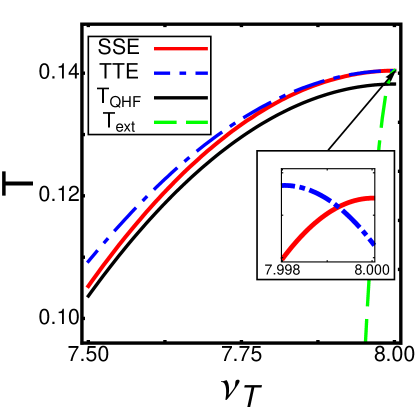
Figure 4: Phase diagram in the $\nu_{T}-T$ plane when energy levels are degenerate. Temperature is in units $\frac{e^{2}}{4\pi\epsilon l_{0}k_{B}}$. $T_{\mathrm{ext}}$ is the extrapolation of the line separating the TTE and SSE phases to low temperature. MoessnerChalker Inset: The SSE phase has a slightly higher ordering temperature than the TTE phase in a very narrow range around $\nu_{T}=8.00$.

For each of the mixed states we find numerically that the order parameters $\Delta_{1}$ and $\Delta_{2}$ do not have the same phase. This can be understood by considering the lowest order term in the free energy that contains $\Delta_{1}$ and $\Delta_{2}$ (see Appendix B):

$$\delta\mathcal{F}_{\mathbf{Q}_{1}=\mathbf{Q}_{2}}^{\left(2\right)} = P_{1}P_{2}U_{12}\left(Q\right)\left[1+U_{11}\left(Q\right)f^{\prime}\left(E_{1}-\mu\right)+U_{22}\left(Q\right)f^{\prime}\left(E_{2}-\mu\right)\right]|\Delta_{1}||\Delta_{2}|\cos\left(\delta\phi_{12}\right).$$ (42)

Here, $\delta\phi_{12}$ is the relative phase between the order parameters. The term in Eq. (42) changes sign at $T=T_{12}=\nu_{1}\left(1-\nu_{1}\right)U_{11}\left(Q_{12}\right)+\nu_{2}\left(1-\nu_{2}\right)U_{22}\left(Q_{12}\right)$. Since $U_{12}\left(Q_{12}\right)$ is negative for the values of $Q_{12}$ that minimize the free energy near the transition, the sign of this term below $T_{12}$ depends on the sign of $\cos\left(\delta\phi_{12}\right)$. In the SSE state, $\delta\phi_{12}=\pi$, while for the TTE state, $\phi_{2i}-\phi_{1i}=\pi$, $i=1$, 2, 3. Thus, the SSE and TTE CDW states can be thought of as coexisting CDW phases in $\Phi_{1}$ and $\Phi_{2}$ ordered at the same wavevector, but $\pi$ out of phase with one another.

It is possible to determine another characteristic temperature associated with equal wavevector ordering in addition to $T_{12}$. Truncating the free energy to $\mathcal{O}\left(\Delta_{i}^{2}\right)$ and minimizing with respect to both of the order parameters and their relative phases leads to the following quadratic equation whose solution yields a characteristic temperature $T_{m}(Q)$:

$$\left(1-\beta\right)T^{2}-2\left(T_{12}-\beta\frac{T_{1}+T_{2}}{2}\right)T+\left(T_{12}^{2}-\beta T_{1}T_{2}\right) = 0,$$ (43)

where $T_{1}=U_{11}\left(Q\right)\nu_{1}\left(1-\nu_{1}\right)+U_{12}\left(Q\right)^{2}/U_{11}\left(Q\right)\nu_{2}\left(1-\nu_{2}\right)$ (similar for $T_{2}$), $T_{12}$ is defined from Eq. (42), and $\beta=4U_{11}\left(Q\right)U_{22}\left(Q\right)/U_{12}\left(Q\right)^{2}$. Solving Eq. (43) for $T=T_{m}\left(Q\right)$ gives us an estimate of the transition temperature at which equal wavevector CDW ordering becomes relevant. Furthermore, maximizing $T_{m}\left(Q\right)$ with respect to $Q$ gives us the critical value of the wavevector at the transition temperature. When terms beyond Eq. (42) are included in the free energy, it is not possible to obtain an analytical solution as we have above, and a numerical solution is required. $T_{12}$ as defined above is larger than the ordering temperatures we find numerically and the presence of cubic terms in the free energy generically leads to a first order transition to the TTE state.

For the particular example we consider here, at the ordering wavevector $Q$, $U_{11}(Q)/U_{22}(Q)\sim 2$, and we find that the ordering temperature for TTE is marginally higher than the ordering temperature for T1 which is much larger than the ordering temperature for T2. The tendency towards ordering is much stronger in state 1 than state 2, but the small energy gain from out of phase equal wavevector ordering in the two states implies that that the TTE phase has the highest ordering temperature.

IV.3.2 Phase diagram at fixed $\nu_{T}$

An orthogonal trajectory in phase space to that considered in Sec. IV.3.1 is to fix $\nu_{T}$ and then vary $\alpha$ and $T$. As $\alpha$ is varied, the filling fractions of the two states vary, which allows for phase transitions between CDW states at fixed temperature. Away from degeneracy, temperature also tunes the relative filling of the two states, with the filling of the higher energy state going to zero at low temperature. We plot phase diagrams for $\nu_{T}=7.50$ and 8.00. These are shown in Figs. 5 and 6 respectively.

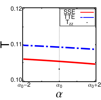
Figure 5: Phase diagram at $\nu_{T}=7.5$ in the $\alpha-T$ plane. Temperature is in units of $\frac{e^{2}}{4\pi\epsilon l_{0}k_{B}}$ and $\alpha$ is dimensionless. The degeneracy point is indicated by a dotted black line on the $\alpha$ axis.

At $\nu_{T}=7.50,$ we see that the TTE phase dominates around the degeneracy point. At $\nu_{T}=8.00$, the SSE state is favoured at values of $\alpha$ close to the degeneracy point, and the TTE phase is favoured away from degeneracy and near the transition temperature. Transitions between triangular and striped phases are first-order in nature. Away from degeneracy and at low enough temperatures, we expect only the state with lowest energy to have non-zero filling, leading to an integer quantum Hall state. The quantum Hall ferromagnetic ordering temperature is below the CDW ordering temperatures in both cases. Similarly to the degenerate case, ordering in state 1 appears to be the main driver of the transition with ordering in state 2 contributing a small lowering of the free energy. The balance of the contribution to ordering of the two states is non-generic and will depend on the details of the two non-interacting states that are participating in the ordering.

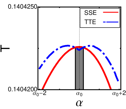
Figure 6: Phase diagram at $\nu_{T}=8.0$ in the $\alpha-T$ plane. Temperature is in units of $\frac{e^{2}}{4\pi\epsilon l_{0}k_{B}}$ and $\alpha$ is dimensionless. The degeneracy point is indicated by a dotted black line on the $\alpha$ axis. The shaded region indicates where SSE ordering is preferred over TTE ordering. Temperature $T_{zz}$ is below the temperature range.

IV.3.3 Generic features of the phase diagram

In our numerical example, we have focused on a particular pair of levels crossing at a particular filling fraction, so it is natural to ask to what extent the features we observe in the phase diagram are generic to when there is Landau level mixing as opposed to specific to the two individual levels that we selected. In general, the choice of two particular levels will affect the coefficients in the Landau theory through the mixing coefficients $C_{\Phi\alpha}$ (as introduced in Eq. (2)). These in turn determine the allowed phases, the ordering temperatures and associated wavevectors, and the relative magnitudes of the relevant order parameters in mixed states. We considered several other crossings in less detail than the one presented here, and these investigations, combined with general expectations, allow us to outline the features we believe to be more or less generic for CDW ordering when there are two levels close to degeneracy. The $\nu_{T}$-$T$ phase diagram we show in Fig. 4 is qualitatively very similar to the temperature-filling phase diagrams found in the case of a single LL by Fogler et al. (FKS)FKS and Moessner and Chalker (MC)MoessnerChalker if we divide $\nu_{0}=\nu_{1}+\nu_{2}$ by 2. In both of these works it was found that for $\nu$ close to $\frac{1}{2}$ in the valence LL, there is a striped CDW, with a transition to a triangular CDW at zero temperature for $\nu_{c}\gtrsim 0.35$ (FKS) or $\nu_{c}\gtrsim 0.39$ (MC). Taking a similar approach, we extrapolate the line separating the SSE and TTE phases in Fig. 4 to zero temperature and find that the SSE phase is stable when the effective filling fraction of each state is approximately $\nu_{c}\gtrsim 0.45$. As MC point out, the perturbative expansion of the free energy is not valid at very low temperatures, so our estimate of $\nu_{c}$ is only approximate. Additionally, we can reasonably expect that the precise estimate of $\nu_{c}$ may depend on which two levels are being studied. In this sense, the results here for degenerate energy levels are consistent with known results on single-LL systems. However, there is an important difference, in that there are effectively two half-filled states and there is co-ordinated ordering in both of them, as opposed to the single half-filled Landau level studied by FKS and MC.

Away from degeneracy the TTE phase tends to be dominant. As $\nu_{0}$ increases towards unity, the SSE phase has a higher transition temperature just near degeneracy. In all of the phases where there is ordering in both states 1 and 2, we observed that the wavevectors ${\mathbf{Q}}_{1}={\mathbf{Q}}_{2}$, which can be understood as arising from the extra free energy that can be gained when the wavevectors are equal in the two states and the order parameters are in phase, as illustrated in Eq. (42).

At degeneracy, we compared the transition temperatures of the CDW states to the QHF states, and found that the system preferred CDW ordering over the QHF ordering. We are uncertain as to the extent to which this behaviour is generic, however, our results appear to indicate that the CDW state can be competitive with quantum Hall ferromagnetism.

V Discussion and Conclusions

We have considered charge density wave ordering in a 2D hole system in a perpendicular magnetic field when Landau level mixing is important. The motivation for this work is recent transport experiments in quantum Hall systems where Landau level mixing was induced by spin-orbit coupling.Manfra ; Grayson Our work is related to the situations investigated by Manfra et al.Manfra and Fischer et al.Grayson There has been some previous theoretical work on both hole striped statesKim and hole FQHE states,Yanghole but these works do not focus on the situation when two levels are close to degenerate and the possible orderings in such a case, as we do here.

Recently, Manfra et al.Manfra studied the transport properties of a two-dimensional hole system in a perpendicular magnetic field. They found anisotropic resistivity at some, but not all, half-integer filling fractions; in particular, they observed isotropic charge transport at $\nu$=9/2, flanked by anisotropic transport at $\nu$=7/2 and $\nu$=11/2. They argue that LL mixing caused by spin-orbit coupling in the valence band of GaAs may be responsible for this pattern of isotropic and anisotropic transport. From a self-consistent calculation of the Landau levels in the Hartree approximation, they suggested that the contribution from the $N=0$ and $N=1$ LLs to the wavefunction of the $\nu=9/2$ state in their particular device likely suppresses the tendency towards charge density wave order.

In Fig. 5 we study the situation in which $\nu_{0}=0.5$ and find that well away from degeneracy so long as there is some occupation of the upper energy level $\nu_{1}\gg\nu_{2}\neq 0$ the effect of LL mixing can be to stabilize a mixed triangular CDW state over the striped CDW state we would expect for an unmixed Landau level. This is another mechanism that could lead to the absence of anisotropic transport at $\nu_{0}=0.5$.

Fischer et al.Grayson observed anomalous transport in the lowest Landau level at what they interpreted to be a field-induced level anti-crossing. At a temperature of 320 mK there was a peak in the longitudinal resistivity that disappeared at 50 mK. As we do not expect our theory to be applicable to the lowest Landau level, we do not speculate on the origin of this anomalous transport. However, we do note that their experiment exhibits a level anti-crossing that occurs because they study a two-dimensional hole rather than a two dimensional electron system. Rashba and Dresselhaus coupling play an important role in determining the energy levels in their device, and if they tuned the Rashba coupling, they would be able to explore the effects of tuning mixing at $\nu_{0}=0.5$ and $\nu_{0}=1$ directly.

Our calculations generalize existing work on 2DEGs in high-LLs to the situation when LL mixing is important, and we show that for a contact potential the Hartree-Fock approximation is exact in the high LL limit even in the presence of LL mixing. We specialize to the situation in which two levels are near the Fermi energy and perform a diagrammatic analysis of the two-particle vertex. This leads us to predict three relevant temperature scales where the uniform system becomes unstable to charge-density wave formation. Two of these correspond to CDW formation in either of the two levels, and the third corresponds to an instability to a mixed CDW phase. Having established a tendency towards CDW ordering, we derive a Landau theory for CDW ordering in the two levels using the Hartree-Fock approximation. We then focus on the specific example of LL mixing induced by Rashba spin-orbit coupling (which could provide a tuning parameter for experimental investigations of the effects of LL mixing on anisotropic transport in the quantum Hall regime).

The effect of Landau level mixing goes beyond changing the character of the single-particle states in the system to also changing the spectrum and the spacing in energy of the single-particle states. We find that it is the second of these that appears to have the most effect on anisotropic quantum Hall states, once the single-particle states have little $N=0$ or 1 character. In particular, at the level of Hartree-Fock, if there are two states relatively near the Fermi energy, only when the filling of one or both states is very close to $\nu=0.5$ is there striped CDW ordering. At other fillings there is triangular CDW ordering. A competing phase when there are two close to degenerate states is that of quantum Hall ferromagnetism, and while in the example we consider here we find the ordering temperature to be less than that for a CDW, thermal fluctuations may treat the two states differently.

We hope that our work stimulates further theoretical and experimental study of anisotropic Quantum Hall states in which externally tuned LL mixing is used as a parameter to investigate the phase diagram.

VI Acknowledgements

The authors thank Igor Herbut and Kun Yang for helpful discussions. This work was supported by NSERC.

Appendix A Full expressions for coefficients in Landau theory

In this Appendix, we give exact expressions for the coefficients in the Landau free energy theory for each case discussed in Sec. III when ${\mathbf{Q}}_{1}\neq{\mathbf{Q}}_{2}$. In solving for the $c_{i}$ and $\gamma$ terms, we determine the chemical potential by setting the number of fermions in the non-interacting system equal to the number of fermions in the interacting system. Then,

$$\mu-\mu_{0} = -\frac{1}{T}\frac{\sum_{kk^{\prime}}\sum_{\left\{\mathbf{Q}_{k}\right\}}P_{k}^{2}\left|U_{kk^{\prime}}\right|^{2}\nu_{k^{\prime}}\left(1-\nu_{k^{\prime}}\right)\left(1-2\nu_{k^{\prime}}\right)\Delta_{k}^{2}}{\sum_{k}\nu_{k}\left(1-\nu_{k}\right)}.$$ (44)

A.1 Mixed unidirectional-unidirectional CDW system

The general form of the free energy for striped phases is

$$\mathcal{F} = P_{1}^{2}a_{1}\left(\mathbf{Q}_{1},T\right)\left|\Delta_{1}\right|^{2}+P_{2}^{2}a_{2}\left(\mathbf{Q}_{2},T\right)\left|\Delta_{2}\right|^{2}+P_{1}^{4}c_{1}\left(\mathbf{Q}_{1},T\right)\left|\Delta_{1}\right|^{4}+P_{2}^{4}c_{2}\left(\mathbf{Q}_{2},T\right)\left|\Delta_{2}\right|^{4}$$ (45)

$$+P_{1}^{2}P_{2}^{2}\gamma\left(\mathbf{Q}_{1},\mathbf{Q}_{2},\theta,T\right)\left|\Delta_{1}\right|^{2}\left|\Delta_{2}\right|^{2},$$

Note that terms involving $\Delta_{i}^{3}$ are not allowed by symmetry. The parameters for the free energy theory in the case of mixed unidirectional-unidirectional CDW ordering are

$$a_{iS}\left(\mathbf{Q}_{i},T\right) = U_{ii}\left(Q_{i}\right)+U_{ii}\left(Q_{i}\right)^{2}f^{\prime}\left(E_{i}-\mu\right)+\sum_{j\neq i}U_{ij}\left(Q_{i}\right)^{2}f^{\prime}\left(E_{j}-\mu\right),$$ (46)

$$c_{iS}\left(\mathbf{Q}_{i},T\right) = \frac{1}{4}\Biggl{[}U_{ii}\left(Q_{i}\right)^{4}f^{\prime\prime\prime}\left(E_{i}-\mu\right)+\sum_{j\neq i}U_{ij}\left(Q_{i}\right)^{4}f^{\prime\prime\prime}\left(E_{j}-\mu\right)\Biggr{]}$$ (47)

$$-\frac{2}{\sum_{k}f^{\prime}\left(E_{k}-\mu\right)}\biggl{\{}U_{ii}\left(Q_{i}\right)^{4}f^{\prime\prime}\left(E_{i}-\mu\right)^{2}+\sum_{j\neq i}\bigl{[}U_{ij}\left(Q_{i}\right)^{4}f^{\prime\prime}\left(E_{j}-\mu\right)^{2}$$

$$\qquad+\,2U_{ii}\left(Q_{i}\right)^{2}U_{ij}\left(Q_{j}\right)f^{\prime\prime}\left(E_{i}-\mu\right)f^{\prime\prime}\left(E_{j}-\mu\right)\bigr{]}\biggr{\}},$$

and

$$\gamma_{SS}\left(\mathbf{Q}_{1},\mathbf{Q}_{2},T\right) = \frac{1}{3}U_{11}\left(Q_{1}\right)U_{12}\left(Q_{2}\right)^{2}f^{\prime\prime\prime}\left(E_{1}-\mu\right)\biggl{[}2+\cos\left(\tilde{Q}_{1}Q_{2}\sin\theta\right)\biggr{]}$$ (48)

$$+\frac{1}{3}U_{12}\left(Q_{1}\right)^{2}U_{22}\left(Q_{2}\right)^{2}f^{\prime\prime\prime}\left(E_{2}-\mu\right)\biggl{[}2+\cos\left(Q_{1}Q_{2}\sin\theta\right)\biggr{]}$$

$$-\frac{1}{\sum_{i}f^{\prime}\left(E_{i}-\mu\right)}\biggl{[}f^{\prime\prime}\left(E_{1}-\mu\right)f^{\prime\prime}\left(E_{2}-\mu\right)U_{11}\left(Q_{1}\right)^{2}U_{22}\left(Q_{2}\right)^{2}$$

$$\qquad\qquad+f^{\prime\prime}\left(E_{1}-\mu\right)^{2}U_{11}\left(Q_{1}\right)^{2}U_{12}\left(Q_{2}\right)^{2}+f^{\prime\prime}\left(E_{2}-\mu\right)^{2}U_{12}\left(Q_{1}\right)^{2}U_{22}\left(Q_{2}\right)^{2}$$

$$\qquad\qquad+f^{\prime\prime}\left(E_{1}-\mu\right)f^{\prime\prime}\left(E_{2}-\mu\right)U_{12}\left(Q_{1}\right)^{2}U_{21}\left(Q_{2}\right)^{2}\biggr{]}.$$

A.2 Mixed triangular-triangular CDW

The free energy when there is mixed triangular-triangular ordering is

$$\mathcal{F} = P_{1}^{2}a_{1}\left(\mathbf{Q}_{1},T\right)\left|\Delta_{1}\right|^{2}+P_{2}^{2}a_{2}\left(\mathbf{Q}_{2},T\right)\left|\Delta_{2}\right|^{2}+P_{1}^{3}b_{1}\left(\mathbf{Q}_{1},T\right)\left|\Delta_{1}\right|^{3}+P_{2}^{3}b_{2}\left(\mathbf{Q}_{1},T\right)\left|\Delta_{2}\right|^{3}$$ (49)

$$+\hskip 2.84544ptP_{1}^{4}c_{1}\left(\mathbf{Q}_{1},T\right)\left|\Delta_{1}\right|^{4}+P_{2}^{4}c_{2}\left(\mathbf{Q}_{2},T\right)\left|\Delta_{2}\right|^{4}+P_{1}^{2}P_{2}^{2}\gamma\left(\mathbf{Q}_{1},\mathbf{Q}_{2},\theta,T\right)\left|\Delta_{1}\right|^{2}\left|\Delta_{2}\right|^{2},$$

A triangular CDW is described by a set of three wavevectors $\left\{\mathbf{Q}_{k}^{j}\right\}_{j=1}^{3}$ lying on a circle of radius $Q_{k}$ oriented $\frac{2\pi}{3}$ radians apart. Allowing for non-collinear CDW ordering between two triangular CDW states, we define $\theta$ as the angle between wavevectors $\mathbf{Q}_{1}^{1}$ and $\mathbf{Q}_{2}^{1}$. Then, the angle between any two wavevectors in $\Phi_{1}$ and $\Phi_{2}$ is $\theta\left(\mathbf{Q}_{1}^{j},\mathbf{Q}_{2}^{j^{\prime}}\right)=\theta+\frac{2\pi}{3}\left(j^{\prime}-j\right).$ There are three possible angles between wavevectors: $\left\{\theta_{i}\right\}_{i=1}^{3}=\left\{\theta,\theta+\frac{2\pi}{3},\theta-\frac{2\pi}{3}\right\}$.

The parameters in this free energy model are

$$a_{iT}\left(\mathbf{Q}_{i},T\right) = 3\Biggl{[}U_{ii}\left(Q_{i}\right)+U_{ii}\left(Q_{i}\right)^{2}f^{\prime}\left(E_{i}-\mu\right)+\sum_{j\neq i}U_{ij}\left(Q_{i}\right)^{2}f^{\prime}\left(E_{j}-\mu\right)\Biggr{]},$$ (50)

$$b_{i}\left(\mathbf{Q}_{i},T\right) = -2\cos\left(\frac{\sqrt{3}Q_{i}^{2}}{4}\right)\Biggl{[}U_{ii}\left(Q_{i}\right)^{3}f^{\prime\prime}\left(E_{i}-\mu\right)+\sum_{j\neq i}U_{ij}\left(Q_{i}\right)^{3}f^{\prime\prime}\left(E_{j}-\mu\right)\Biggr{]},$$ (51)

$$c_{iT}\left(\mathbf{Q}_{i},T\right) = \frac{15}{4}U_{ii}\left(Q_{i}\right)^{4}f^{\prime\prime\prime}\left(E_{i}-\mu\right)-U_{ii}\left(Q_{i}\right)^{4}f^{\prime\prime\prime}\left(E_{i}-\mu\right)\Biggl{[}1-\cos\left(\frac{\sqrt{3}}{2}Q_{i}^{2}\right)\Biggr{]}$$ (52)

$$+\sum_{j\neq i}\Biggl{\{}\frac{15}{4}U_{ij}\left(Q_{i}\right)^{4}f^{\prime\prime\prime}\left(E_{j}-\mu\right)-U_{ij}\left(Q_{i}\right)^{4}f^{\prime\prime\prime}\left(E_{j}-\mu\right)\Biggl{[}1-\cos\left(\frac{\sqrt{3}}{2}Q_{i}^{2}\right)\Biggr{]}\Biggr{\}}$$

$$-\frac{9}{2\sum_{i}f^{\prime}\left(E_{i}-\mu\right)}\biggl{\{}U_{ii}\left(Q_{i}\right)^{4}f^{\prime\prime}\left(E_{i}-\mu\right)^{2}$$

$$\qquad+\sum_{j\neq i}\biggl{[}f^{\prime\prime}\left(E_{j}-\mu\right)^{2}U_{ij}\left(Q_{i}\right)+2f^{\prime\prime}\left(E_{i}-\mu\right)f^{\prime\prime}\left(E_{j}-\mu\right)U_{ii}\left(Q_{i}\right)^{2}U_{ij}\left(Q_{i}\right)\biggr{]}\biggr{\}},$$

and

$$\gamma_{TT}\left(\mathbf{Q}_{1},\mathbf{Q}_{2},T\right) = \left[U_{11}\left(Q_{1}\right)^{2}U_{12}\left(Q_{2}\right)^{2}f^{\prime\prime\prime}\left(E_{1}-\mu\right)+U_{11}\left(Q_{1}\right)^{2}U_{12}\left(Q_{2}\right)^{2}f^{\prime\prime\prime}\left(E_{1}-\mu\right)\right]$$ (53)

$$\times\biggl{\{}6+\cos\left(Q_{1}Q_{2}\sin\theta\right)+\cos\left[Q_{1}Q_{2}\sin\left(\theta+\frac{2\pi}{3}\right)\right]+\cos\left[Q_{1}Q_{2}\sin\left(\theta-\frac{2\pi}{3}\right)\right]\biggr{\}}$$

$$-\frac{9}{\sum_{i}f^{\prime}\left(E_{i}-\mu\right)}\biggl{[}f^{\prime\prime}\left(E_{1}-\mu\right)f^{\prime\prime}\left(E_{2}-\mu\right)U_{11}\left(Q_{1}\right)^{2}U_{22}\left(Q_{2}\right)^{2}$$

$$\qquad+f^{\prime\prime}\left(E_{1}-\mu\right)^{2}U_{11}\left(Q_{1}\right)^{2}U_{12}\left(Q_{2}\right)^{2}+f^{\prime\prime}\left(E_{2}-\mu\right)^{2}U_{12}\left(Q_{1}\right)^{2}U_{22}\left(Q_{2}\right)^{2}$$

$$\qquad+f^{\prime\prime}\left(E_{1}-\mu\right)f^{\prime\prime}\left(E_{2}-\mu\right)U_{12}\left(Q_{1}\right)^{2}U_{22}\left(Q_{2}\right)^{2}\biggr{]}.$$

A.3 Mixed unidirectional-triangular CDW

Without loss of generality, assume that there is unidirectional CDW ordering in $\Phi_{1}$ and triangular CDW ordering in $\Phi_{2}$. Then the free energy is

$$\mathcal{F} = P_{1}^{2}a_{1}\left(\mathbf{Q}_{1},T\right)\left|\Delta_{1}\right|^{2}+P_{2}^{2}a_{2}\left(\mathbf{Q}_{2},T\right)\left|\Delta_{2}\right|^{2}+P_{2}^{3}b_{2}\left(\mathbf{Q}_{1},T\right)\left|\Delta_{2}\right|^{3}$$ (54)

$$+P_{1}^{4}c_{1}\left(\mathbf{Q}_{1},T\right)\left|\Delta_{1}\right|^{4}+P_{2}^{4}c_{2}\left(\mathbf{Q}_{2},T\right)\left|\Delta_{2}\right|^{4}+P_{1}^{2}P_{2}^{2}\hskip 2.84544pt\gamma\left(\mathbf{Q}_{1},\mathbf{Q}_{2},\theta,T\right)\left|\Delta_{1}\right|^{2}\left|\Delta_{2}\right|^{2},$$

All coefficients except $\gamma$ remain unchanged for each type of ordering. The coupling parameter is

$$\gamma_{ST}\left(\mathbf{Q}_{1},\mathbf{Q}_{2},T\right) = \frac{1}{3}\left[U_{11}\left(Q_{1}\right)^{2}U_{12}\left(Q_{2}\right)^{2}f^{\prime\prime\prime}\left(E_{1}-\mu\right)\right.+\left.U_{11}\left(Q_{1}\right)^{2}U_{12}\left(Q_{2}\right)^{2}f^{\prime\prime\prime}\left(E_{1}-\mu\right)\right]$$ (55)

$$\qquad\times\biggl{\{}6+\cos\left(Q_{1}Q_{2}\sin\theta\right)+\cos\left[Q_{1}Q_{2}\sin\left(\theta+\frac{2\pi}{3}\right)\right]+\cos\left[Q_{1}Q_{2}\sin\left(\theta-\frac{2\pi}{3}\right)\right]\biggr{\}}$$

$$-\frac{3}{\sum_{i}f^{\prime}\left(E_{i}-\mu\right)}\biggl{[}f^{\prime\prime}\left(E_{1}-\mu\right)f^{\prime\prime}\left(E_{2}-\mu\right)U_{11}\left(Q_{1}\right)^{2}U_{22}\left(Q_{2}\right)^{2}$$

$$\qquad+f^{\prime\prime}\left(E_{1}-\mu\right)^{2}U_{11}\left(Q_{1}\right)^{2}U_{12}\left(Q_{2}\right)^{2}+f^{\prime\prime}\left(E_{2}-\mu\right)^{2}U_{12}\left(Q_{1}\right)^{2}U_{22}\left(Q_{2}\right)^{2}$$

$$\qquad+f^{\prime\prime}\left(E_{1}-\mu\right)f^{\prime\prime}\left(E_{2}-\mu\right)U_{12}\left(Q_{1}\right)^{2}U_{22}\left(Q_{2}\right)^{2}\biggr{]}.$$

Appendix B Full expressions for coefficients in Landau theory when ${\mathbf{Q}}_{1}={\mathbf{Q}}_{2}$

In the previous appendix we gave exact expressions for the coefficients in the Landau free energy theory for each case discussed in Sec. III. When the ordering wavevectors ${\mathbf{Q}}_{1}={\mathbf{Q}}_{2}={\mathbf{Q}}$ then there are additional terms in the free energy, as described in Eq. (34) as $\delta{\mathcal{F}}_{{\mathbf{Q}}_{1}={\mathbf{Q}}_{2}}$. We give expressions for the coefficients in Eq. (34) in this Appendix.

B.1 Mixed unidirectional-unidirectional CDW system

The extra terms that appear in the free energy theory for SSE ordering are of the form

$$\delta f_{SSE} = P_{1}P_{2}\alpha_{SSE}\left(Q,\delta\phi,T\right)\left|\Delta_{1}\right|\left|\Delta_{2}\right|+P_{1}^{3}P_{2}\sigma_{SSE}\left(Q,\delta\phi,T\right)\left|\Delta_{1}\right|^{3}\left|\Delta_{2}\right|$$ (56)

$$+P_{1}^{2}P_{2}^{2}\gamma_{SSE}\left(Q,\delta\phi,T\right)\left|\Delta_{1}\right|^{2}\left|\Delta_{2}\right|^{2}+P_{1}P_{2}^{3}\rho_{SSE}\left(Q,\delta\phi,T\right)\left|\Delta_{1}\right|\left|\Delta_{2}\right|^{3}.$$

Here, $Q$ is the magnitude of the ordering wavevector, $\delta\phi$ the relative phase between order parameters $\Delta_{1}\left(\mathbf{Q}\right)$ and $\Delta_{2}\left(\mathbf{Q}\right)$, and $T$ the temperature. The values of the coefficients are

$$\alpha_{SSE}\left(Q,\delta\phi,T\right) = 2U_{12}\left(Q\right)\biggl{[}1+U_{11}\left(Q\right)f^{\prime}\left(E_{1}-\mu\right)+U_{22}\left(Q\right)f^{\prime}\left(E_{2}-\mu\right)\biggr{]}\cos\left(\delta\phi\right),$$ (57)

$$\sigma_{SSE}\left(Q,\delta\phi,T\right) = \biggl{\{}U_{11}\left(Q\right)^{3}U_{12}\left(Q\right)f^{\prime\prime\prime}\left(E_{1}-\mu\right)+U_{12}\left(Q\right)^{3}U_{11}\left(Q\right)f^{\prime\prime\prime}\left(E_{2}-\mu\right)$$ (58)

$$\qquad-\frac{1}{\sum_{i=1}^{2}f^{\prime}\left(E_{i}-\mu\right)}\left[U_{11}\left(Q\right)^{2}f^{\prime\prime}\left(E_{1}-\mu\right)+U_{12}\left(Q\right)^{2}f^{\prime\prime}\left(E_{2}-\mu\right)\right]$$

$$\qquad\times\left[U_{11}\left(Q\right)U_{12}\left(Q\right)f^{\prime\prime}\left(E_{1}-\mu\right)+U_{22}\left(Q\right)U_{12}\left(Q\right)f^{\prime\prime}\left(E_{2}-\mu\right)\right]\biggr{\}}\cos\left(\delta\phi\right),$$

$$\gamma_{SSE}\left(Q,\delta\phi,T\right) = \biggl{\{}\frac{1}{2}\biggl{[}U_{11}\left(Q\right)^{2}U_{12}\left(Q\right)^{2}f^{\prime\prime\prime}\left(E_{1}-\mu\right)+U_{12}\left(Q\right)^{2}U_{22}\left(Q\right)^{2}f^{\prime\prime\prime}\left(E_{2}-\mu\right)\biggr{]}$$ (59)

$$\qquad-\frac{1}{\sum_{i=1}^{2}f^{\prime}\left(E_{i}-\mu\right)}$$

$$\qquad\times\left[U_{11}\left(Q\right)U_{12}\left(Q\right)f^{\prime\prime}\left(E_{1}-\mu\right)+U_{22}\left(Q\right)U_{12}\left(Q\right)f^{\prime\prime}\left(E_{2}-\mu\right)\right]^{2}\biggr{\}}\left[1+2\cos^{2}\left(\delta\phi\right)\right]$$

$$-\frac{1}{\sum_{i=1}^{2}f^{\prime}\left(E_{i}-\mu\right)}\left[U_{11}\left(Q\right)U_{22}\left(Q\right)-U_{12}\left(Q\right)^{2}\right]^{2}f^{\prime\prime}\left(E_{1}-\mu\right)f^{\prime\prime}\left(E_{2}-\mu\right),$$

and

$$\rho_{SSE}\left(Q,\delta\phi,T\right) = \biggl{\{}U_{11}\left(Q\right)U_{12}\left(Q\right)^{3}f^{\prime\prime\prime}\left(E_{1}-\mu\right)+U_{12}\left(Q\right)U_{22}\left(Q\right)^{3}f^{\prime\prime\prime}\left(E_{2}-\mu\right)$$ (60)

$$\qquad-\frac{1}{\sum_{i=1}^{2}f^{\prime}\left(E_{i}-\mu\right)}\left[U_{22}\left(Q\right)^{2}f^{\prime\prime}\left(E_{2}-\mu\right)+U_{12}\left(Q\right)^{2}f^{\prime\prime}\left(E_{1}-\mu\right)\right]$$

$$\qquad\times\left[U_{11}\left(Q\right)U_{12}\left(Q\right)f^{\prime\prime}\left(E_{1}-\mu\right)+U_{22}\left(Q\right)U_{12}\left(Q\right)f^{\prime\prime}\left(E_{2}-\mu\right)\right]^{2}\biggr{\}}\cos\left(\delta\phi\right).$$

B.2 Mixed triangular-triangular CDW system

The order parameter for the triangular CDW state depends on a set of three wavevectors, $\left\{\mathbf{Q}_{i}^{\alpha}\right\}_{\alpha=1}^{3}$. We associate ordering at each wavevector with a particular phase $\phi_{i}^{\alpha}$, such that $\Delta_{i}\left(\mathbf{Q}_{i}^{\alpha}\right)=\Delta_{i}e^{i\phi_{\iota}^{\alpha}}$. Thus, when $\mathbf{Q}_{1}=\mathbf{Q}_{2}$, we end up with six new parameters to consider when minimizing the free energy. We may reduce the number of parameters from six to four in the following manner (where $i=1,\,2,\,3$):

$$\delta\phi_{i} = \phi_{1}^{i}-\phi_{2}^{i},$$ (61)

$$\tilde{\phi}_{1} = \sum_{i=1}^{3}\phi_{1}^{i},$$ (62)

$$\tilde{\phi}_{2} = \tilde{\phi}_{1}-\sum_{i=1}^{3}\delta\phi_{i}$$ (63)

The new terms in the free energy theory for TTE ordering are

$$\delta f_{TTE} = P_{1}P_{2}\alpha_{TTE}\left(Q,\delta\phi_{1},\delta\phi_{2},\delta\phi_{3},T\right)\left|\Delta_{1}\right|\left|\Delta_{2}\right|+P_{1}^{2}P_{2}\eta_{TTE}\left(Q,\delta\phi_{1},\delta\phi_{2},\delta\phi_{3},\tilde{\phi}_{1},T\right)\left|\Delta_{1}\right|^{2}\left|\Delta_{2}\right|$$ (64)

$$+P_{1}P_{2}^{2}\varphi_{TTE}\left(Q,\delta\phi_{1},\delta\phi_{2},\delta\phi_{3},\tilde{\phi}_{2},T\right)\left|\Delta_{1}\right|\left|\Delta_{2}\right|^{2}+P_{1}^{3}P_{2}\sigma_{TTE}\left(Q,\delta\phi_{1},\delta\phi_{2},\delta\phi_{3},T\right)\left|\Delta_{1}\right|^{3}\left|\Delta_{2}\right|$$

$$+P_{1}^{2}P_{2}^{2}\gamma_{TTE}\left(Q,\delta\phi_{1},\delta\phi_{2},\delta\phi_{3},T\right)\left|\Delta_{1}\right|^{2}\left|\Delta_{2}\right|^{2}+P_{1}P_{2}^{3}\rho_{TTE}\left(Q,\delta\phi_{1},\delta\phi_{2},\delta\phi_{3},T\right)\left|\Delta_{1}\right|\left|\Delta_{2}\right|^{3}.$$

Here, $Q$ is the magnitude of the ordering wavevector, $\delta\phi$ the relative phase between order parameters $\Delta_{1}\left(\mathbf{Q}\right)$ and $\Delta_{2}\left(\mathbf{Q}\right)$, and $T$ the temperature. The values of the coefficients are

$$\alpha_{TTE}\left(Q,\delta\phi_{1},\delta\phi_{2},\delta\phi_{3},T\right) = U_{12}\left(Q\right)\biggl{[}1+U_{11}\left(Q\right)f^{\prime}\left(E_{1}-\mu\right)+U_{22}\left(Q\right)f^{\prime}\left(E_{2}-\mu\right)\biggr{]}\sum_{i=1}^{3}\cos\left(\delta\phi_{i}\right),$$ (65)

$$\eta_{TTE}\left(Q,\delta\phi_{1},\delta\phi_{2},\delta\phi_{3},\tilde{\phi}_{1},T\right) = -6\biggl{[}U_{11}\left(Q\right)^{2}U_{12}\left(Q\right)f^{\prime\prime}\left(E_{1}-\mu\right)+U_{11}\left(Q\right)U_{12}\left(Q\right)^{2}f^{\prime\prime}\left(E_{2}-\mu\right)\biggr{]}$$ (66)

$$\times\cos\left(\frac{\sqrt{3}}{4}Q^{2}\right)\sum_{i=1}^{3}\cos\left(\tilde{\phi}_{1}-\delta\phi_{i}\right),$$

$$\varphi_{TTE}\left(Q,\delta\phi_{1},\delta\phi_{2},\delta\phi_{3},\tilde{\phi}_{1},T\right) = -6\biggl{[}U_{12}\left(Q\right)^{2}U_{11}\left(Q\right)f^{\prime\prime}\left(E_{1}-\mu\right)+U_{12}\left(Q\right)U_{22}\left(Q\right)^{2}f^{\prime\prime}\left(E_{2}-\mu\right)\biggr{]}$$ (67)

$$\times\cos\left(\frac{\sqrt{3}}{4}Q^{2}\right)\sum_{i=1}^{3}\cos\left(\tilde{\phi}_{2}+\delta\phi_{i}\right),$$

$$\sigma_{TTE}\left(Q,\delta\phi,T\right) = \biggl{\{}\frac{1}{3}\left[11+4\cos\left(\frac{\sqrt{3}}{2}Q^{2}\right)\right]\left[U_{11}\left(Q\right)^{3}U_{12}\left(Q\right)f^{\prime\prime\prime}\left(E_{1}-\mu\right)+U_{22}\left(Q\right)U_{12}\left(Q\right)^{3}f^{\prime\prime\prime}\left(E_{2}-\mu\right)\right]$$ (68)

$$\qquad-\frac{6}{\sum_{i=1}^{2}f^{\prime}\left(E_{i}-\mu\right)}\left[U_{11}\left(Q\right)U_{12}\left(Q\right)f^{\prime\prime}\left(E_{1}-\mu\right)+U_{22}\left(Q\right)U_{12}\left(Q\right)f^{\prime\prime}\left(E_{2}-\mu\right)\right]^{2}$$

$$\qquad\times\biggl{[}U_{11}\left(Q\right)^{2}+U_{12}\left(Q\right)^{2}\biggr{]}\biggr{\}}\sum_{\alpha}\cos\left(\phi_{1\alpha}-\phi_{2\alpha}\right),$$

$$\gamma_{TTE}\left(Q,\delta\phi,T\right) = \biggl{\{}\frac{1}{2}\biggl{[}U_{11}\left(Q\right)^{2}U_{12}\left(Q\right)^{2}f^{\prime\prime\prime}\left(E_{1}-\mu\right)+U_{12}\left(Q\right)^{2}U_{22}\left(Q\right)^{2}f^{\prime\prime\prime}\left(E_{2}-\mu\right)\biggr{]}$$ (69)

$$\qquad-\frac{1}{\sum_{i=1}^{2}f^{\prime}\left(E_{i}-\mu\right)}\left[U_{11}\left(Q\right)U_{12}\left(Q\right)f^{\prime\prime}\left(E_{1}-\mu\right)+U_{22}\left(Q\right)U_{12}\left(Q\right)f^{\prime\prime}\left(E_{2}-\mu\right)\right]^{2}\biggr{\}}$$

$$\times\sum_{i=1}^{3}\left[1+2\cos^{2}\left(\delta\phi_{i}\right)\right]$$

$$+\biggl{\{}\frac{2}{3}\biggl{[}U_{11}\left(Q\right)^{2}U_{12}\left(Q\right)^{2}f^{\prime\prime\prime}\left(E_{1}-\mu\right)+U_{12}\left(Q\right)^{2}U_{22}\left(Q\right)^{2}f^{\prime\prime\prime}\left(E_{2}-\mu\right)\biggr{]}$$

$$\qquad\times\left[2+\cos\left(\frac{\sqrt{3}}{2}Q^{2}\right)\right]-\frac{2}{\sum_{i=1}^{2}f^{\prime}\left(E_{i}-\mu\right)}$$

$$\qquad\times\left[U_{11}\left(Q\right)U_{12}\left(Q\right)f^{\prime\prime}\left(E_{1}-\mu\right)+U_{22}\left(Q\right)U_{12}\left(Q\right)f^{\prime\prime}\left(E_{2}-\mu\right)\right]^{2}\biggr{\}}$$

$$\times\sum_{i=1}^{3}\sum_{j\neq i}\left[1+2\cos\left(\delta\phi_{i}\right)\cos\left(\delta\phi_{j}\right)\right]$$

$$-\frac{9}{\sum_{i=1}^{2}f^{\prime}\left(E_{i}-\mu\right)}\left[U_{11}\left(Q\right)U_{22}\left(Q\right)-U_{12}\left(Q\right)^{2}\right]^{2}f^{\prime\prime}\left(E_{1}-\mu\right)f^{\prime\prime}\left(E_{2}-\mu\right),$$

and

$$\rho_{TTE}\left(Q,\delta\phi,T\right) = \biggl{\{}\frac{1}{3}\left[11+4\cos\left(\frac{\sqrt{3}}{2}Q^{2}\right)\right]\left[U_{12}\left(Q\right)^{3}U_{22}\left(Q\right)f^{\prime\prime\prime}\left(E_{2}-\mu\right)+U_{11}\left(Q\right)U_{12}\left(Q\right)^{3}f^{\prime\prime\prime}\left(E_{1}-\mu\right)\right]$$ (70)

$$\qquad-\frac{6}{\sum_{i=1}^{2}f^{\prime}\left(E_{i}-\mu\right)}\left[U_{11}\left(Q\right)U_{12}\left(Q\right)f^{\prime\prime}\left(E_{1}-\mu\right)+U_{22}\left(Q\right)U_{12}\left(Q\right)f^{\prime\prime}\left(E_{2}-\mu\right)\right]$$

$$\qquad\times\biggl{[}U_{12}\left(Q\right)^{2}+U_{22}\left(Q\right)^{2}\biggr{]}\biggr{\}}\sum_{\alpha}\cos\left(\phi_{1\alpha}-\phi_{2\alpha}\right).$$

B.3 Mixed unidirectional-triangular CDW system

We consider mixing between a unidirectional phase in $\Phi_{1}$ and a triangular phase in $\Phi_{2}$. Without loss of generality, we let $\mathbf{Q}_{1}=\mathbf{Q}_{2}^{1}$. Thus, we end up with two new parameters:

$$\delta\phi = \phi_{1}-\phi_{2},$$ (71)

$$\tilde{\phi}_{2} = \sum_{i=1}^{3}\phi_{2}^{i},$$ (72)

The new terms in the free energy theory for STE ordering are

$$\delta f_{STE} = P_{1}P_{2}\alpha_{STE}\left(Q,\delta\phi,T\right)\left|\Delta_{1}\right|\left|\Delta_{2}\right|+P_{1}P_{2}^{2}\varphi_{STE}\left(Q,\delta\phi,\tilde{\phi}_{2},T\right)\left|\Delta_{1}\right|\left|\Delta_{2}\right|^{2}+P_{1}^{2}P_{2}^{2}\gamma_{STE}\left(Q,\delta\phi,T\right)\left|\Delta_{1}\right|^{2}\left|\Delta_{2}\right|^{2}$$ (73)

$$+P_{1}^{3}P_{2}\sigma_{STE}\left(Q,\delta\phi,T\right)\left|\Delta_{1}\right|^{3}\Delta_{2}+P_{1}P_{2}^{3}\rho_{TTE}\left(Q,\delta\phi,T\right)\left|\Delta_{1}\right|\left|\Delta_{2}\right|^{3}.$$

The coefficients are

$$\alpha_{STE}\left(Q,\delta\phi,T\right) = 2U_{12}\left(Q\right)\biggl{[}1+U_{11}\left(Q\right)f^{\prime}\left(E_{1}-\mu\right)+U_{22}\left(Q\right)f^{\prime}\left(E_{2}-\mu\right)\biggr{]}\cos\left(\delta\phi\right),$$ (74)

$$\varphi_{STE}\left(Q,\delta\phi,\tilde{\phi}_{2},T\right) = -2\biggl{[}U_{12}\left(Q\right)^{2}U_{11}\left(Q\right)f^{\prime\prime}\left(E_{1}-\mu\right)+U_{12}\left(Q\right)U_{22}\left(Q\right)^{2}f^{\prime\prime}\left(E_{2}-\mu\right)\biggr{]}$$ (75)

$$\times\cos\left(\frac{\sqrt{3}}{4}Q^{2}\right)\cos\left(\tilde{\phi}_{2}+\delta\phi\right),$$

$$\sigma_{STE}\left(Q,\delta\phi,T\right) = \biggl{\{}\frac{1}{3}\left[19+8\cos\left(\frac{\sqrt{3}}{2}Q^{2}\right)\right]\left[U_{11}\left(Q\right)^{3}U_{12}\left(Q\right)f^{\prime\prime\prime}\left(E_{1}-\mu\right)+U_{22}\left(Q\right)U_{12}\left(Q\right)^{3}f^{\prime\prime\prime}\left(E_{2}-\mu\right)\right]$$ (76)

$$\qquad-\frac{1}{\sum_{i=1}^{2}f^{\prime}\left(E_{i}-\mu\right)}\left[U_{11}\left(Q\right)U_{12}\left(Q\right)f^{\prime\prime}\left(E_{1}-\mu\right)+U_{22}\left(Q\right)U_{12}\left(Q\right)f^{\prime\prime}\left(E_{2}-\mu\right)\right]^{2}$$

$$\qquad\times\biggl{(}U_{11}\left(Q\right)^{2}+U_{12}\left(Q\right)^{2}\biggr{)}\biggr{\}}\cos\left(\delta\phi\right),$$

$$\gamma_{STE}\left(Q,\delta\phi,T\right) = \biggl{\{}\frac{1}{2}U_{11}\left(Q\right)^{2}U_{12}\left(Q\right)^{2}f^{\prime\prime\prime}\left(E_{1}-\mu\right)+U_{12}\left(Q\right)^{2}U_{22}\left(Q\right)^{2}f^{\prime\prime\prime}\left(E_{2}-\mu\right)$$ (77)

$$\qquad-\frac{1}{\sum_{i=1}^{2}f^{\prime}\left(E_{i}-\mu\right)}\left[U_{11}\left(Q\right)U_{12}\left(Q\right)f^{\prime\prime}\left(E_{1}-\mu\right)+U_{22}\left(Q\right)U_{12}\left(Q\right)f^{\prime\prime}\left(E_{2}-\mu\right)\right]^{2}\biggr{\}}$$

$$\times\left[1+\frac{2}{3}\cos^{2}\left(\delta\phi\right)\right]$$

$$+\biggl{\{}\left[3+2\cos\left(\frac{\sqrt{3}}{2}Q^{2}\right)\right]U_{11}\left(Q\right)^{2}U_{12}\left(Q\right)^{2}f^{\prime\prime\prime}\left(E_{1}-\mu\right)+U_{12}\left(Q\right)^{2}U_{22}\left(Q\right)^{2}f^{\prime\prime\prime}\left(E_{2}-\mu\right)$$

$$\qquad-\frac{3}{\sum_{i=1}^{2}f^{\prime}\left(E_{i}-\mu\right)}\left[U_{11}\left(Q\right)U_{12}\left(Q\right)f^{\prime\prime}\left(E_{1}-\mu\right)+U_{22}\left(Q\right)U_{12}\left(Q\right)f^{\prime\prime}\left(E_{2}-\mu\right)\right]^{2}\biggr{\}},$$

and

$$\rho_{STE}\left(Q,\delta\phi,T\right) = \biggl{\{}\frac{1}{3}\left[19+8\cos\left(\frac{\sqrt{3}}{2}Q^{2}\right)\right]\left[U_{12}\left(Q\right)^{3}U_{22}\left(Q\right)f^{\prime\prime\prime}\left(E_{2}-\mu\right)+U_{11}\left(Q\right)U_{12}\left(Q\right)^{3}f^{\prime\prime\prime}\left(E_{1}-\mu\right)\right]$$ (78)

$$\qquad-\frac{1}{\sum_{i=1}^{2}f^{\prime}\left(E_{i}-\mu\right)}\left[U_{11}\left(Q\right)U_{12}\left(Q\right)f^{\prime\prime}\left(E_{1}-\mu\right)+U_{22}\left(Q\right)U_{12}\left(Q\right)f^{\prime\prime}\left(E_{2}-\mu\right)\right]$$

$$\qquad\times\biggl{[}U_{12}\left(Q\right)^{2}+U_{22}\left(Q\right)^{2}\biggr{]}\biggr{\}}\cos\left(\delta\phi\right).$$

Appendix C Hartree-Fock potentials for quantum Hall ferromagnets

In this appendix, we derive expressions for the potentials $W_{IJ}$ in the Hartree-Fock approximation. We use notation similar to Sec. III, but note that lower-case letters label the individual states $\Phi_{i}$ while upper-case letters label the pseudospin indices. Let

$$F_{ij}\left(\mathbf{q}\right) = \sum_{\alpha}C_{i\alpha}^{*}C_{j\alpha}e^{-i\left(n_{i\alpha}-n_{j\alpha}\right)\left(\theta-\pi/2\right)}A_{n_{i\alpha}n_{j\alpha}}\left[\frac{\left(ql_{0}\right)^{2}}{2}\right],$$ (79)

where

$$A_{mn}\left(x\right) = \sqrt{\frac{m!}{n!}}x^{\frac{n-m}{2}}\mathcal{L}_{m}^{n-m}\left(x\right),\mbox{ }m\leq n.$$

Then

$$\rho\left(\mathbf{q}\right) = e^{-\frac{\left(ql_{0}\right)^{2}}{4}}\sum_{ij=1}^{2}F_{ij}\left(\mathbf{q}\right)\sum_{X}e^{-iq_{x}X}a_{iX_{+}}^{\dagger}a_{jX_{-}}$$

We invert Eq. (37) to solve for $a_{iX_{+}}^{\dagger}a_{jX_{-}}$ in terms of the $\hat{m}_{I,\mathbf{q}}$ operators and rewrite $\rho\left(\mathbf{q}\right)$ as follows:

$$\rho\left(\mathbf{q}\right) = e^{-\frac{\left(ql_{0}\right)^{2}}{4}}\sum_{IJ=0,x,y,z}\mathcal{F}_{I}\left(\mathbf{q}\right)\hat{m}_{I,\mathbf{q}},$$

where $\mathcal{F}_{I}\left(\mathbf{q}\right)=\frac{1}{2}\sigma_{I}^{\left(ij\right)}F_{ij}\left(\mathbf{q}\right)$. The density-density Hamiltonian is then

$$H_{QHF} = \frac{1}{2}\sum_{\mathbf{q}}\sum_{IJ}e^{-\frac{\left(ql_{0}\right)^{2}}{2}}{V_{IJ}\left(\mathbf{q}\right)}\hat{m}_{I,\mathbf{q}}\hat{m}_{J,-\mathbf{q}},$$ (80)

where ${V_{IJ}\left(\mathbf{q}\right)}={v\left(\mathbf{q}\right)}{\mathcal{F}_{I}\left(\mathbf{q}\right)}{\mathcal{F}_{j}\left(-\mathbf{q}\right)}$, ${v\left(\mathbf{q}\right)}$ being the electron-electron interaction potential.

We apply the HF approximation to Eq. (80) to obtain Eq. (39). The HF potentials $W_{IJ}$ are defined as follows:

$${W_{00}} = \frac{1}{2\pi}\int{\rm d}^{2}\mathbf{q}\,e^{-\frac{\left(ql_{0}\right)^{2}}{2}}\left[{V_{00}\left(\mathbf{q}\right)}-{V_{00}\left(0\right)}-\frac{1}{2}{u\left(\mathbf{q}\right)}\right],$$

$${W_{II}} = \frac{1}{2\pi}\int{\rm d}^{2}\mathbf{q}\,e^{-\frac{\left(ql_{0}\right)^{2}}{2}}\left[{V_{II}\left(\mathbf{q}\right)}-{V_{II}\left(0\right)}+\frac{1}{2}{u\left(\mathbf{q}\right)}\right],$$

$${W_{IJ}} = \frac{1}{2\pi}\int{\rm d}^{2}\mathbf{q}\,e^{-\frac{\left(ql_{0}\right)^{2}}{2}}\left[{V_{IJ}\left(\mathbf{q}\right)}-{V_{IJ}\left(0\right)}\right],$$

where

$${u\left(\mathbf{q}\right)} = {F_{11}\left(\mathbf{q}\right)}{F_{22}\left(\mathbf{q}\right)}-{F_{12}\left(\mathbf{q}\right)}{F_{21}\left(\mathbf{q}\right)}.$$

For each potential, conservation of LL index in the basis state interactions must be observed. Thus, for the eigenstates considered in Sec. IV, the only nonzero potentials are $W_{00}$, $W_{zz}$, $W_{0z}=W_{z0}$, and $W_{xx}=W_{yy}$.

References

- (1) K. von Klitzing, G. Dorda, M. Pepper, Phys. Rev. Lett. 45, 494 (1980).
- (2) D.C. Tsui, H.L. Strmer, A.C. Gossard, Phys. Rev. Lett. 48, 1559 (1982).
- (3) R.E. Prange and S.M. Girvin (eds.), The Quantum Hall effect, Springer-Verlag, New York (1987).
- (4) B.I. Halperin, P.A. Lee, and N. Read, Phys. Rev. B 47, 7312 (1993).
- (5) G. Moore and N. Read, Nucl. Phys. B 360, 362 (1991).
- (6) R. Willett, J.P. Eisenstein, H.L. Stormer, D. C. Tsui, A.C. Gossard, and J.H. English, Phys. Rev. Lett. 59, 1776 (1987).
- (7) M.P. Lilly, K.B. Cooper, J.P. Eisenstein, L.N. Pfeiffer, and K.W. West, Phys. Rev. Lett. 82, 394 (1999).
- (8) W. Pan, R. R. Du, H. L. Stormer, D. C. Tsui, L. N. Pfeiffer, K. W. Baldwin, and K. W. West, Phys. Rev. Lett. 83, 820 (1999).
- (9) M. P. Lilly, K. B. Cooper, J. P. Eisenstein, L. N. Pfeiffer, and K. W. West, Phys. Rev. Lett. 83, 824 (1999).
- (10) H. Fukuyama, P.M. Platzman, and P.W. Anderson, Phys. Rev. B 19, 5211 (1979).
- (11) A.A. Koulakov, M.M. Fogler, and B.I. Shklovskii, Phys. Rev. Lett. 76, 499 (1996).
- (12) R. Moessner and J.T. Chalker, Phys. Rev. B 54, 5006 (1996).
- (13) M. M. Fogler, A. A. Koulakov, and B. I. Shklovskii, Phys. Rev. B 54, 1853 (1996).
- (14) M. M. Fogler and A. A. Koulakov, Phys. Rev. B 55, 9326 (1997).
- (15) E. Fradkin and S.A. Kivelson, Phys. Rev. B 59, 8065 (1999).
- (16) E.H. Rezayi, F.D. M. Haldane, and K. Yang, Phys. Rev. Lett. 83, 1219 (1999).
- (17) A. H. MacDonald and M. P. A. Fisher, Phys. Rev. B 61, 5724 (2000).
- (18) E. Fradkin, S. A. Kivelson, E. Manousakis, and K. Nho, Phys. Rev. Lett. 84, 1982 (2000).
- (19) C. Wexler and A. T. Dorsey, Phys. Rev. B 64, 115312 (2001).
- (20) L. Radzihovsky and A. T. Dorsey, Phys. Rev. Lett. 88, 216802 (2002).
- (21) D. G. Barci, E. Fradkin, S. A. Kivelson, and V. Oganesyan, Phys. Rev. B 65, 245319 (2002).
- (22) Q. M. Doan and E. Manousakis, Phys. Rev. B 75, 195433 (2007).
- (23) E. Fradkin, arXiv:1004.1104v1.
- (24) H. Zhu, G. Sambandamurthy, L.W. Engel, D.C. Tsui, L.N. Pfeiffer, and K.W. West, Phys. Rev. Lett. 102, 136804 (2009).
- (25) O. Ciftja, J. Appl. Phys. 107, 09C504 (2010).
- (26) M.J. Manfra, R. de Picciotto, Z. Jiang, S.H. Simon, L.N. Pfeiffer, K.W. West, and A.M. Sergent, Phys. Rev. Lett. 98, 206804 (2007).
- (27) G.M. Gusev, A.K. Bakarov, T.E. Lamas, and J.C. Portal, Phys. Rev. Let. 99, 126804 (2007).
- (28) F. Fischer, R. Winkler, D. Schuh, M. Bichler, and M. Grayson, Phys. Rev. B 75, 073303 (2007).
- (29) R. Winkler, Spin-Orbit Coupling Effects in two-dimensional Electron and Hole Systems (Springer-Verlag, New York, 2003).
- (30) A.H. MacDonald, Phys. Rev. B 30, 4392 (1984).
- (31) T.D. Stanescu, I. Martin, and P. Phillips, Phys. Rev. Lett. 84, 1288 (2000).
- (32) G.A. Csathy, H. Noh, D.C. Tsui, L.N. Pfeiffer, and K.W. West, Phys. Rev. Lett. 94, 226802 (2005).
- (33) S.H. Simon, Phys. Rev. Lett. 100, 116803 (2008).
- (34) W. Bishara and C. Nayak, Phys. Rev. B 80, 121302(R) (2009).
- (35) S. Chesi and D. Loss, Phys. Rev. Lett. 101, 146803 (2008).
- (36) M.E. Raikh and T.V. Shahbazyan, Phys. Rev. B 47, 1522 (1993).
- (37) R.R. Gerhardts, Phys. Rev. B 24, 1339 (1981); R.R. Gerhardts, Phys. Rev. B 24, 4068 (1981).
- (38) M. Rasolt, B. I. Halperin, and D. Vanderbilt, Phys. Rev. Lett. 57, 126 (1986).
- (39) Y. Imry, J. Phys. C: Solid State Phys. 5, 567 (1975).
- (40) M. Levinshtein, S. Rumyantsev, and M. Shur, Handbook Series on Semiconductor Parameters (World Scientific, River Edge, 1996), Vol. 1, Chap. 4.
- (41) S. Schmult, C. Gerl, U. Wurstbauer, C. Mitzkus, and W. Wegscheider, Appl. Phys. Lett. 86, 202105 (2005).
- (42) I.L. Aleiner and L.I. Glazman, Phys. Rev. B. 52, 11296 (1995).
- (43) A. H. MacDonald, P. M. Platzman, and G. S. Boebinger, Phys. Rev. Lett. 65, 775 (1990).
- (44) T. Jungwirth and A. H. MacDonald, Phys. Rev. B 63, 035305 (2000).
- (45) T.-S. Kim, S.-R.E. Yang, and A.H. MacDonald, Phys. Rev. B 62, R7747 (2000).
- (46) S.-R.E. Yang, A.H. MacDonald, and D. Yoshioka, Phys. Rev. B 41, R1290 (1990).