Spitzer Analysis of Hii Region Complexes in the Magellanic Clouds:
Determining a Suitable Monochromatic Obscured Star Formation Indicator

Abstract

Hii regions are the birth places of stars, and as such they provide the best measure of current star formation rates (SFRs) in galaxies. The close proximity of the Magellanic Clouds allows us to probe the nature of these star forming regions at small spatial scales. To study the Hii regions, we compute the bolometric infrared flux, or total infrared (TIR), by integrating the flux from 8 to 500 $\mu$m. The TIR provides a measure of the obscured star formation because the UV photons from hot young stars are absorbed by dust and re-emitted across the mid-to-far-infrared (IR) spectrum. We aim to determine the monochromatic IR band that most accurately traces the TIR and produces an accurate obscured SFR over large spatial scales. We present the spatial analysis, via aperture/annulus photometry, of 16 Large Magellanic Cloud (LMC) and 16 Small Magellanic Cloud (SMC) Hii region complexes using the Spitzer Space Telescope’s IRAC (3.6, 4.5, 8 $\mu$m) and MIPS (24, 70, 160 $\mu$m) bands. Ultraviolet rocket data (1500 and 1900 Å) and SHASSA H$\alpha$ data are also included. All data are convolved to the MIPS 160 $\mu$m resolution (40 arcsec full width at half-maximum), and apertures have a minimum radius of $35\arcsec$. The IRAC, MIPS, UV, and H$\alpha$ spatial analysis are compared with the spatial analysis of the TIR. We find that nearly all of the LMC and SMC Hii region spectral energy distributions (SEDs) peak around 70 $\mu$m at all radii, from $\sim 10$ to $\sim 400$ pc from the central ionizing sources. As a result, we find the following: the sizes of Hii regions as probed by 70 $\mu$m is approximately equal to the sizes as probed by TIR ($\approx 70$ pc in radius); the radial profile of the 70 $\mu$m flux, normalized by TIR, is constant at all radii (70 $\mu\mbox{m}\sim 0.45~{}\mbox{TIR}$); the $1\sigma$ standard deviation of the 70 $\mu$m fluxes, normalized by TIR, is a lower fraction of the mean ($0.05-0.12$ out to $\sim 220$ pc) than the normalized 8, 24, and 160 $\mu$m normalized fluxes ($0.12-0.52$); and these results are the same for the LMC and the SMC. From these results, we argue that 70 $\mu$m is the most suitable IR band to use as a monochromatic obscured star formation indicator because it most accurately reproduces the TIR of Hii regions in the LMC and SMC and over large spatial scales. We also explore the general trends of the 8, 24, 70, and 160 $\mu$m bands in the LMC and SMC Hii region SEDs, radial surface brightness profiles, sizes, and normalized (by TIR) radial flux profiles. We derive an obscured SFR equation that is modified from the literature to use 70 $\mu$m luminosity, $\mbox{SFR}~{}(M_{\odot}~{}\mbox{yr}^{-1})=9.7(0.7)\times 10^{-44}~{}L_{70}~{}(\mbox{ergs}~{}\mbox{s}^{-1})$, which is applicable from 10 to 300 pc distance from the center of an Hii region. We include an analysis of the spatial variations around Hii regions between the obscured star formation indicators given by the IR and the unobscured star formation indicators given by UV and H$\alpha$. We compute obscured and unobscured SFRs using equations from the literature and examine the spatial variations of the SFRs around Hii regions.

1. INTRODUCTION

Hii regions are locations of active or recent star formation where the extreme ultraviolet (UV) radiation from massive OB stars ionizes the surrounding gas (for a good review see chapter 5 of Tielens, 2005, and references therein). It is common to consider Hii regions as being large complexes of overlapping individual Hii regions where the sizes and components are not determined solely by the classical Strömgren radius of an individual star but by an inclusion of all of the physical regimes in the interstellar medium (ISM) affected by the far-UV photons of the central sources. These Hii region components include the central ionizing OB stars, and the surrounding photodissociation regions (PDRs) and molecular clouds, where the chemistry and the heating are driven by the UV photons from nearby stars (Tielens, 2005; Relaño & Kennicutt, 2009; Watson et al., 2008). Thus, Hii regions in this context are really Hii complexes, or more generally, star forming regions.

The observed properties of these star forming regions, including size and shape, depend on the physical traits such as the number of young hot ionizing stars, density of neutral gas, abundance of dust, star formation history, and prior supernovae (e.g., see Hodge, 1974; Tielens, 2005; Walborn et al., 2002; Snider et al., 2009; Harris & Zaritsky, 2009). These physical traits are often correlated, and the use of data at many wavelengths to observe Hii regions in different galactic environments is required to piece them together.

The nature of the hot central OB stars can be studied using UV (e.g., Smith et al., 1987; Martin et al., 2005) or nebular emission lines, such as H$\alpha$ (e.g., Henize, 1956; Hodge & Kennicutt, 1983; Gaustad et al., 2001). The H$\alpha$ luminosity function of a galaxy is frequently used to determine many of the physical properties of Hii regions, including the number of ionizing stars, evolutionary effects, and possible environmental effects (Kennicutt et al., 1989; Oey & Clarke, 1998). Hii region size distributions are directly related to the luminosity functions and relate to the numbers of nebula of a given size for a galaxy(e.g., van den Bergh, 1981; Oey et al., 2003). The PDRs can be studied by many methods including the [Oi] and [Cii] infrared (IR) cooling lines and CO radio data (e.g., Kaufman et al., 1999). The molecular clouds are typically studied using radio observations of molecular rotational lines (e.g., Cohen et al., 1988; Genzel, 1991; Fukui et al., 2008).

Present star formation rates (SFRs) are calculated using a tracer of the UV photons from the young massive stars and spectral synthesis models (see Kennicutt, 1998). Hii regions will have some fraction of their UV photons obscured by dust and some fraction unobscured. For unobscured SFRs, the ionizing photons can be directly observed via UV observations or recombination lines such as H$\alpha$. For obscured Hii regions, bolometric IR observations of dust (i.e., the total infrared (TIR)) can be used to recover the extinguished UV photons. This is because the dust absorption cross section is highly peaked in the UV, and the re-emitted flux is in the broad spectral range from the mid-to-far-IR (Kennicutt, 1998). Because the TIR around Hii regions accounts for all of the extincted UV photons, the TIR is expected to be the single best indicator of SFR obscured by dust.

Combining UV, optical, and IR observations of Hii regions across a whole galaxy allows us to probe the current SFR of that galaxy. The Large Magellanic Cloud (LMC) and Small Magellanic Cloud (SMC) are ideal natural laboratories for studying star forming regions and their effects on the ISM. The close proximities of the LMC and SMC, at $\sim 52$ kpc (Szewczyk et al., 2008) and $\sim 60$ kpc (Hilditch et al., 2005), respectively, allow for detailed star formation studies down to parsec or sub-parsec scales depending on wavelength. Any broad study of Hii regions across the LMC and SMC can take advantage of many multiwavelength observations, including the rocket UV data from Smith et al. (1987), the Southern H$\alpha$ Sky Survey Atlas (SHASSA) H$\alpha$ data from Gaustad et al. (2001), and the Spitzer Space Telescope IR data from Meixner et al. (2006) and K. D. Gordon et al. (2010, in preparation). Furthermore, there are many past optical Hii region surveys that catalog the sources of H$\alpha$ in the LMC and SMC (see Henize, 1956; Davies et al., 1976; Bica & Schmitt, 1995).

Because of the observational advantages, many researchers rely on a single-band star formation indicator (i.e., UV, H$\alpha$, Pa$\alpha$, 8 $\mu$m, 24 $\mu$m, etc). There are complications in the UV and optical lines in that they can be greatly impacted by extinction, thus, requiring extinction corrections. Another complication is that the observed UV photons can come from stars of various ages ($<100$ Myr) and will greatly depend on galaxy type (i.e., quiescent spiral galaxies, starbursts, etc.; (Calzetti et al., 2005)). The 8 and 24 $\mu$m IR band emission will likely depend on the environment of the host galaxy because the abundance of the aromatics/small grains that give rise to their emission depend upon the metallicity and ionizing radiation present (K. D. Gordon et al. 2010, in preparation; Draine & Li, 2007; Draine et al., 2007). Work done by Calzetti et al. (2007) and Dale et al. (2005) indicate that 8 $\mu$m makes for a poor star formation indicator due to large variability of emission in galaxies with respect to spectral energy distribution (SED) shape and metallicity. Calzetti et al. (2007) also note, along with Calzetti et al. (2005), that a star formation indicator using 24 $\mu$m by itself can vary from galaxy to galaxy. Dale et al. (2005) claim that SFRs calculated from 24 $\mu$m emission may be off by a factor of 5 due to variations of 24 $\mu$m flux with respect to SEDs observed across nearby galaxies.

To compensate for the extinction effects in UV and optical nebular emission lines, many researchers are now measuring SFRs via a combination of obscured (TIR, 8 $\mu$m, 24 $\mu$m) and unobscured (UV, H$\alpha$, Pa$\alpha$) star formation indicators (e.g., Calzetti et al., 2007; Kennicutt et al., 2007; Thilker et al., 2007; Relaño & Kennicutt, 2009; Kennicutt et al., 2009). However, the noted differences in 8 and 24 $\mu$m emission, relative to host galaxy properties, may still introduce uncertainties to the calculated SFRs when applying them across large galaxy samples. In their analysis of 33 galaxies from the Spitzer SINGS sample, Calzetti et al. (2007) claim that a combination of H$\alpha$ and 24 $\mu$m gives the most robust SFR using a procedure similar to the Gordon et al. (2000) “flux ratio method”. Their calibration has a caveat in that it is useful for actively star forming galaxies where the energy output is dominated by young stellar populations (Calzetti et al., 2007). Kennicutt et al. (2009) analyze SFRs of nearby galaxies derived by combining H$\alpha$ with 8 $\mu$m, 24 $\mu$m, and the TIR. They find that linear combinations of H$\alpha$ and TIR provide for the most robust SFRs.

There is little work done on investigating the efficacy of using 70 or 160 $\mu$m as star formation indicators. Dale et al. (2005) claim that the 70 $\mu$m emission may make a good monochromatic obscured star formation indicator because the 70 to 160 $\mu$m ratio correlates well with local SFRs. A Spitzer analysis of far-IR compact sources in the LMC (van Loon et al., 2010a) and SMC (van Loon et al., 2010b), including compact Hii regions, find that the bolometric correction to 70 $\mu$m is modest, due to a typical dust temperature of 40 K. In a study of dwarf irregular galaxies, Walter et al. (2007) find a good correlation between the brightest 70 $\mu$m regions and optical tracers of star formation, albeit, with some galaxies contributing significant 70 $\mu$m diffuse emission at large radii.

Which of the Spitzer IR bands most accurately reproduces the TIR over a large spatial scale? Employing aperture/annulus photometry, we analyze 16 LMC and 16 SMC Hii region complexes using the Spitzer Infrared Array Camera (IRAC) and Multiband Imaging Photometer (MIPS) bands. We determine that the MIPS 70 $\mu$m band provides for the most accurate monochromatic obscured star formation indicator based on an analysis of the Hii region complex SEDs, sizes, and radial monochromatic IR fluxes (normalized by the TIR). We include an analysis of the spatial distribution of the unobscured star formation indicators, UV and H$\alpha$, relative to the IR obscured star formation indicators. We modify an established TIR SFR recipe from Kennicutt (1998) to derive a new monochromatic obscured SFR equation using the 70 $\mu$m luminosity.

In Section 2, we list the LMC and SMC Hii region complexes sampled in this work. In Section 3, we explain the IR, UV, and H$\alpha$ observations and data reduction. The analysis of the multiwavelength photometry is discussed in Section 4. The basic results of the photometry, SEDs, and radial profiles, are discussed in Section 5 as well as a discussion of our calculation of the TIR. Discussions of Hii region normalized radial SEDs, Hii complex sizes, normalized radial profiles, and SFRs are presented in Section 6. In this section we also present our derived 70 $\mu$m obscured SFR equation. We finish with some concluding statements in Section 7.

2. Hii REGION SAMPLE

The 16 LMC and 16 SMC Hii regions were selected by the following three criteria: the center must be peaked in 24 $\mu$m emission, there must be a nearby peak in H$\alpha$, and the total sample of Hii regions must sample the full size of the LMC and SMC as observed in 24 $\mu$m. Along with sampling Hii regions across the entire LMC and SMC, the 16 LMC and 16 SMC Hii regions cover a wide range of sizes and temperatures. The final sample size is a compromise between obtaining good statistics and avoiding overlap between the large apertures covering each Hii region. Specifics of the Hii regions are listed in Table 1. The maximum radii are chosen to include the full extent of the Hii region complex. We describe how we quantify this in section 4.1 and 6.2.

Table 1Sample of Hii Regions

		$\alpha$ (2000)	$\delta$ (2000)	Maximum Radius
No.	Namea	(h:m:s)	(∘:$\arcmin$:$\arcsec$)	($\arcsec$)	(pc)b
LMC
1	N4	4:52:08	-66:55:20	1120	280
2	N11	4:56:48	-66:24:41	1505	380
3	N30	5:13:51	-67:27:22	875	220
4	N44	5:22:12	-67:58:31	980	250
5	N48	5:25:50	-66:15:03	1470	370
6	N55	5:32:33	-66:27:20	910	230
7	N59	5:35:23	-67:34:46	875	220
8	N79	4:51:54	-69:23:29	560	140
9	N105	5:09:52	-68:52:59	1785	450
10	N119	5:18:40	-69:14:27	980	250
11	N144	5:26:47	-68:48:48	455	115
12	N157	5:38:36	-69:05:33	1225	310
13	N160	5:39:44	-69:38:47	805	205
14	N180	5:48:38	-70:02:04	1015	255
15	N191	5:04:39	-70:54:34	525	130
16	N206	5:31:22	-71:04:10	1400	355
SMC
1	DEM74	0:53:14	-73:12:18	350	105
2	N13	0:45:23	-73:22:52	350	105
3	N17	0:46:42	-73:31:04	385	115
4	N19	0:48:26	-73:05:59	385	115
5	N22	0:48:09	-73:14:56	350	105
6	N36	0:50:31	-72:52:30	525	155
7	N50	0:53:26	-72:42:56	560	165
8	N51	0:52:40	-73:26:29	350	105
9	N63	0:58:17	-72:38:57	350	105
10	N66	0:59:06	-72:10:44	700	205
11	N71	1:00:59	-71:35:30	490	145
12	N76	1:03:43	-72:03:19	350	105
13	N78	1:05:06	-71:59:36	350	105
14	N80	1:08:34	-71:59:43	560	165
15	N84	1:14:05	-73:17:04	980	290
16	N90	1:29:35	-73:33:44	385	115

Shown in Figures 1 and 2 are LMC and SMC images of the unobscured and obscured star formation indicators of UV (blue–LMC only), H$\alpha$ (green contours), and 24 $\mu$m (red). The Hii regions are labeled with circles denoting the maximum extent to which we measure their photometry (see Columns 5 and 6 in Table 1). We do not have UV data for the SMC. A more detailed discussion of these figures is presented in section 6.4. For full Spitzer IRAC and MIPS images of the entire LMC and SMC, see Meixner et al. (2006), K. D. Gordon et al. (2010, in preparation), van Loon et al. (2010a), and van Loon et al. (2010b).

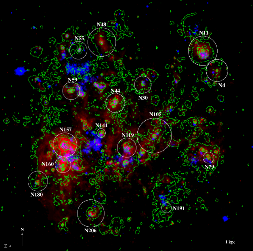
Figure 1.— LMC image of the UV (blue) from Smith et al. (1987), H$\alpha$ (green contours) from Gaustad et al. (2001), and 24 $\mu$m (red) from Meixner et al. (2006). UV and 24 $\mu$m are convolved to the MIPS 160 $\mu$m resolution ($40\arcsec$). The SHASSA H$\alpha$ fluxes are in their original resolution ($\sim 45\arcsec$). The selected Hii regions are labeled and marked with an aperture that corresponds to the largest spatial extent for which we measure the photometry (see Table 1). The bar in the lower right represents 1 kpc. North is up, and east is to the left.

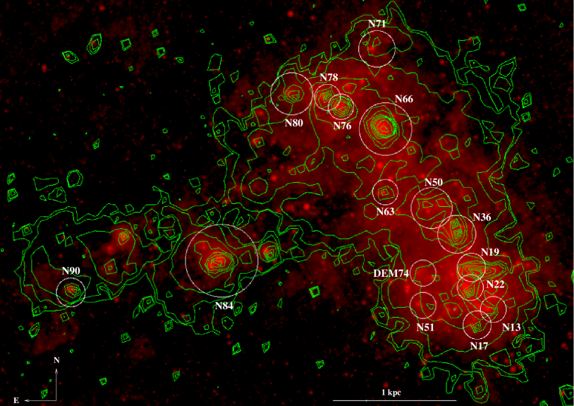
Figure 2.— SMC image of the H$\alpha$ (green contours) from Gaustad et al. (2001) and 24 $\mu$m (red) from K. D. Gordon et al. (2010, in preparation). The 24 $\mu$m fluxes are convolved to the MIPS 160 $\mu$m resolution ($40\arcsec$). The SHASSA H$\alpha$ fluxes are in their original resolution ($\sim 45\arcsec$). The selected Hii regions are labeled and marked with an aperture that corresponds to the largest spatial extent for which we measure the photometry (see Table 1). The bar in the lower right represents 1 kpc. North is up, and east is to the left.

To view the dust structure of the Hii regions, three-color images of the LMC Hii regions are shown in Figure 3. The SMC Hii region three-color dust images are shown in Figure 4. In both figures, the aromatic 8 $\mu$m emission is in blue, the warm 24 $\mu$m dust emission is green, and the colder 160 $\mu$m dust emission is red. The sizes of the Hii regions span from 105 pc in radius to 450 pc in radius. Although we describe the 8 $\mu$m emission as aromatic, we do not attempt to remove any possible non-aromatic components. The IRAC 8 $\mu$m band may have some contamination from emission of lines such as Hi, [Arii], and [Ariii] (Peeters et al., 2002; Lebouteiller et al., 2007). A more detailed discussion is presented in section 5.3.

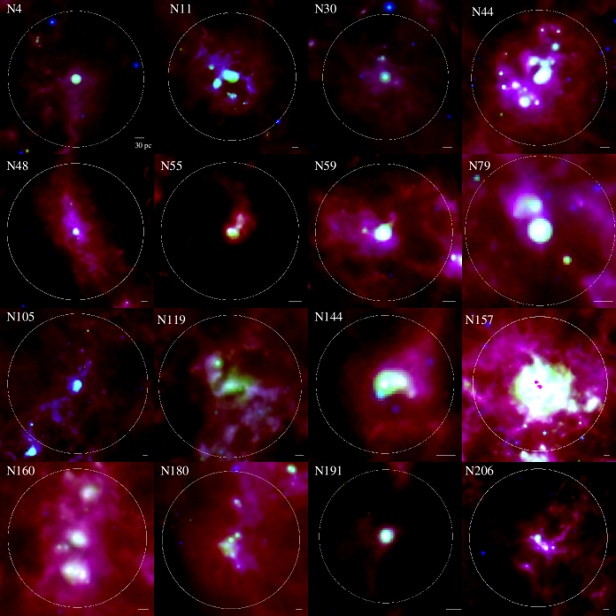
Figure 3.— Three-color dust images of the 16 LMC Hii regions using the IRAC and MIPS data from Meixner et al. (2006). The IRAC 8 $\mu$m is blue, the MIPS 24 $\mu$m is green, and the coldest dust at the MIPS 160 $\mu$m band is red. The 8 and 24 $\mu$m fluxes are convolved to the MIPS 160 $\mu$m resolution ($40\arcsec$). The bars in the lower right of each image represent 30 pc. The white circles represent the largest apertures used for the photometry (see Table 1). North is up and east is to the left. The lack of 24 $\mu$m flux in the center of 30 Doradus (N157) is due to saturation in the core.

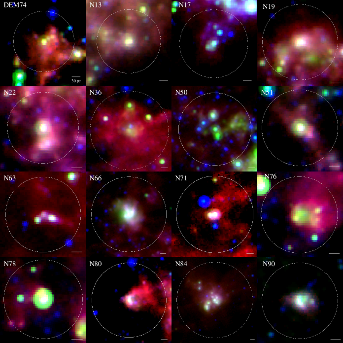
Figure 4.— Three-color dust images of the 16 SMC Hii regions using the IRAC and MIPS data from K. D. Gordon et al. (2010, in preparation). The IRAC 8 $\mu$m is blue, the MIPS 24 $\mu$m is green, and the coldest dust at the MIPS 160 $\mu$m is red. The 8 and 24 $\mu$m fluxes are convolved to the MIPS 160 $\mu$m resolution ($40\arcsec$). The bars in the lower right of each image represent 30 pc. The white circles represent the largest apertures used for the photometry (see Table 1). North is up and east is to the left.

3. OBSERVATIONS

3.1. IR

The infrared images are created from the Spitzer Space Telescope’s IRAC and MIPS instruments for the Surveying the Agents of a Galaxy’s Evolution (SAGE) project (see Werner et al. 2004; Meixner et al. 2006; K. D. Gordon et al. 2010, in preparation). The observations and data reductions are fully described in the SAGE LMC overview paper (Meixner et al., 2006) and in the SAGE SMC overview paper (K. D. Gordon et al. 2010, in preparation).

IRAC provides MIR imaging data in four passbands centered around 3.6 $\mu$m, 4.5 $\mu$m, 5.8 $\mu$m, and 8 $\mu$m (Fazio et al., 2004). MIPS provides FIR imaging data in three passbands centered around 24 $\mu$m, 70 $\mu$m, and 160 $\mu$m (Rieke et al., 2004). The LMC and SMC IRAC exposures consist of $1\fdg 1\times 1\fdg 1$ tiles. The LMC MIPS exposures are scan legs $4\,^{\circ}$ long, and the SMC MIPS exposures are scan legs $2\,^{\circ}-5\,^{\circ}$ long. The exposure depths are the same for both galaxies as a result of the same observing strategies, and variations between the IRAC tiles and MIPS strips have been removed. The observations were taken at two epochs separated by $\sim 3$ (LMC/IRAC, LMC/MIPS, SMC/IRAC) and $\sim 9$ (SMC/MIPS) months.

The full mosaics, for each IRAC and MIPS band, are created via processing using the Wisconsin pipeline (IRAC; see description in Meixner et al., 2006) and the MIPS DAT analysis tool (MIPS; Gordon et al., 2005). The background has been subtracted from the full mosaics of each galaxy to remove zodiacal and Milky Way cirrus emission. The mosaics cover $\sim 8\,^{\circ}\times 8\,^{\circ}$ for the LMC and $\sim 30$ deg² for the SMC.

The angular resolution of the IRAC mosaics are $1\farcs 7$, $1\farcs 7$, $1\farcs 9$, and $2\arcsec$ for the 3.6, 4.5, 5.8, and 8 $\mu$m bands. The angular resolution of the MIPS mosaics are $6\arcsec$, $18\arcsec$, and $40\arcsec$ for the 24, 70, and 160 $\mu$m bands. So that the data have equivalent resolution, all of the IRAC and MIPS point-spread functions (PSFs) have been transformed to the 40″ PSF of the MIPS 160 $\mu$m band using the custom convolution kernels from Gordon et al. (2008).

3.2. ANCILLARY DATA

The UV data are from imaging taken with sounding-rocket intrumentation (Smith et al., 1987). The bandpasses, centered around 1495 Å and 1934 Å, are 200 Å wide full width at half-maximum (FWHM) and 220 Å wide FWHM, respectively (Smith et al., 1987). In this paper, we use 1500 Å and 1900 Å  to refer to these UV bands. The 1500 Å image has a total exposure time of 114s, and the 1900 Å image has a total exposure time of 130s. The 1500 Å PSFs and the 1900 Å PSFs have been convolved to match the 160 $\mu$m PSF using the custom convolution kernels of Gordon et al. (2008).

The H$\alpha$ images are from the southern sky wide-angle imaging survey known as the SHASSA (see Gaustad et al., 2001). The SHASSA survey uses a Canon camera with a 52 mm focal length lens and an H$\alpha$ filter centered at 6563 Å with a 32 Å bandwidth. The LMC and SMC images are each comprised of five separate 20m exposures. The LMC and SMC are in fields 013 and 010 in Gaustad et al. (2001), respectively. SHASSA images have a similar resolution ($\sim 45\arcsec$) to that of the MIPS 160 $\mu$m images ($40\arcsec$).

4. ANALYSIS

4.1. Photometry

The LMC and SMC photometries are measured for the IRAC (3.6 $\mu$m, 4.5 $\mu$m, 8 $\mu$m) bands, MIPS (24 $\mu$m, 70 $\mu$m, 160 $\mu$m) bands, and the ancillary data for all 32 Hii regions spanning physical sizes from $\sim 105$ pc in radius to $\sim 450$ pc in radius (see Table 1 and Figures 3 & 4). The photometry of the Hii regions is measured in concentric annuli from the central inner $35\arcsec$ aperture outward to the annulus with the largest radii. The radii of the annuli are chosen such that they fully sample the PSF and are large enough to attain good signal-to-noise in the outer parts of the Hii regions where the UV, H$\alpha$, and 24 $\mu$m fluxes quickly drop to background levels. The flux for a given annulus is calculated by taking the flux of a larger aperture and subtracting off the flux from the adjacent smaller aperture. From these annuli, we create radial SEDs and radial flux profiles of each Hii region.

The central apertures for each Hii region are centered around the peak 24 $\mu$m flux because the peak 24 $\mu$m flux is observed to closely coincide with the peak H$\alpha$ flux (Relaño & Kennicutt, 2009). Also, the 24 $\mu$m flux is observed to peak around OB stars at spatial scales down to less than a parsec (Snider et al., 2009). Each 24 $\mu$m peak is visually checked to make sure that it coincides with a nearby peak in the H$\alpha$ SHASSA data and in the H$\alpha$ catalog of either Henize (1956) or Davies et al. (1976). An H$\alpha$ peak is considered nearby a 24 $\mu$m peak if it falls within the central three annuli.

The $35\arcsec$ apertures correspond to slightly different physical scales for the LMC and SMC. The LMC is $\sim$52 kpc away (Szewczyk et al., 2008) which corresponds to a physical aperture radius of $\approx 9$ pc. The SMC is $\sim$60.5 kpc away (Hilditch et al., 2005) which corresponds to a physical aperture radius of $\approx 10$ pc. Thus, we are restricted to measuring the properties associated with the dust around Hii regions at scales larger than $\approx 9$ pc for the LMC and $\approx 10$ pc for the SMC.

The largest apertures of the Hii region complexes are determined, by eye, to be where the coldest gas, emitting at 160 $\mu$m, drops in flux to approximately the level of the background diffuse emission or where the Hii region begins to overlap another Hii region. The Hii region complex sizes are more quantitatively determined in section 6.2.

To remove the sky background and the local LMC or SMC background, due to diffuse emission, we perform a background flux removal for each Hii region. The background flux for every annulus of a given Hii region is computed with an annulus taken at radii of 1.1–1.5 times the radius of the largest aperture. The flux error for a given annulus is then the standard deviation of the background sky flux times the square root of the number of pixels in the annulus. In the instances where a neighboring Hii region will fall within the background sky annulus, a mask is created that nulls the pixel values in the background sky annulus where any large 24 $\mu$m peaks are observed. The interloping Hii region is nulled in every band. The SMC is a smaller galaxy with smaller distances between bright Hii regions, relative to the LMC (see Figures 1 and 2). This crowding sets up a lower angular size limit of the maximum aperture used for many of the SMC Hii regions.

We also perform the total IR photometry of each Hii region using an aperture with the largest radius (see Table 1) to acquire the cumulative flux. These fluxes are used to plot the Hii region SEDs in section 5.1. For all cumulative fluxes, the background flux is taken from the same sky annulus as in the photometry of the individual annuli.

The total IR fluxes of the LMC and SMC galaxies are computed using aperture photometry with apertures that enclose each galaxy. The LMC circular aperture is centered around 5${}^{\mbox{h}}$:17${}^{\mbox{m}}$:50${}^{\mbox{s}}$ right ascension and -68^∘:24$\arcmin$:42$\arcsec$ declination (epoch 2000 coordinates) with a 14,100$\arcsec$ radius. The SMC aperture is an ellipse centered around 1${}^{\mbox{h}}$:06${}^{\mbox{m}}$:00${}^{\mbox{s}}$ right ascension and -72^∘:50$\arcmin$:46$\arcsec$ declination (epoch 2000 coordinates) with a major axis radius of 9710$\arcsec$ and a minor axis radius of 9140$\arcsec$. The LMC and SMC sky backgrounds are taken from regions outside of their apertures and away from any bright IRAC/MIPS infrared sources.

The number of Hii regions with a given aperture/annulus decreases considerably with larger radii for both the LMC and SMC. Thus, the conclusions in this work suffer from low number statistics at larger radii. For the LMC, the number of Hii regions drops to five at an aperture/outer annulus radius of $1225\arcsec$. For the SMC, the number drops to five at an aperture/outer annulus radius of $525\arcsec$.

5. RESULTS:

5.1. SEDs

Hii region IR SEDs are a combination of the Rayleigh–Jeans tail of the stellar photospheric emission and emission from dust grain populations. The 3.6 $\mu$m fluxes, and to a lesser degree the 4.5 $\mu$m fluxes, are associated with stellar continua more than dust (Helou et al., 2004). Engelbracht et al. (2008) find that the transition from stellar dominated emission to dust dominated emission in starburst galaxies occurs around 4.5 $\mu$m. The dust emission at 5.8 and 8 $\mu$m is likely dominated by aromatic emission (Puget & Leger, 1989). To more conservatively separate the dust emission from IR emission associated with stellar photospheres, we do not include the 5.8 $\mu$m band in our analysis .

The 24, 70, and 160 $\mu$m FIR emission are associated with silicate and carbonaceous grains of various sizes, as demonstrated by interstellar dust grain models (e.g., Draine & Lee, 1984; Desert et al., 1990; Li & Draine, 2001). Draine & Li (2007) find that small grains, of sizes $\sim 15-40$ Å, may contribute a significant portion of the 24 $\mu$m continuum via single-photon heating. The 70 $\mu$m emission may be due to a significant fraction of both small grains and large grains, but 160$\mu$m fluxes are dominated by large grains (Desert et al., 1990).

From our annulus photometry, we produce IR SEDs for each annulus of each Hii region. Each of these radial Hii region IR SEDs is created by using the fluxes (mJy Hz) at 3.6, 4.5, 8, 24, 70, and 160 $\mu$m. For each Hii region, we analyze the SEDs and compare how they change radially from the core to the outermost measured annulus. A full analysis of the radial SEDs is discussed in section 6.1.

We also produce IR SEDs using the cumulative flux of each Hii region and compare these with the SEDs created using the total galactic LMC and SMC fluxes. The total LMC and SMC fluxes were computed using a single aperture around each galaxy (see section 4.1). The LMC, SMC, and Hii region cumulative fluxes, in Jy, and their $1\sigma$ uncertainties are tabulated in Table 2. The SEDs are plotted in Figure 5$a$ for the LMC, and Figure 5$b$ for the SMC. The maximum aperture radius used for each Hii region correspond to the apertures marked in Figures 3 and 4 and in the last two columns of Table 1.

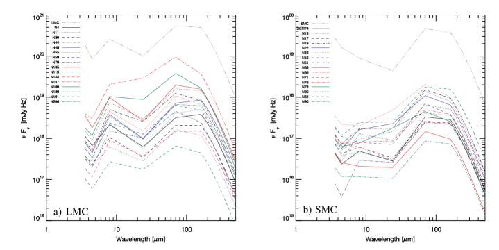
Figure 5.— IR SEDs of the cumulative fluxes (mJy Hz) of the Hii regions (calculated using the largest aperture) in the –a) LMC and –b) SMC. The total galactic LMC and SMC fluxes are also plotted as triple-dot-dashed lines in gray. The computation of the Rayleigh–Jeans tail (160-500 $\mu$m) is explained in Section 5.2.

Table 2IR Fluxes of Hii Regions

Name	$3.6\mu$m	$4.5\mu$m	$8\mu$m	$24\mu$m	$70\mu$m	$160\mu$m	$T_{\mbox{c}}^{a}$
	(Jy)	(Jy)	(Jy)	(Jy)	(Jy)	(Jy)	(K)
LMC
LMCb	$2150\pm 40$	$1280\pm 20$	$6860\pm 140$	$8080\pm 320$	$127000\pm 6400$	$265000\pm 32000$	23.9
N4	$13.4\pm 0.24$	$9.88\pm 0.19$	$57.3\pm 1.2$	$49.5\pm 2.0$	$742\pm 37$	$2040\pm 240$	22.6
N11	$17.8\pm 0.33$	$13.6\pm 0.3$	$198\pm 4$	$238\pm 10$	$3730\pm 190$	$7700\pm 920$	23.9
N30	$4.44\pm 0.10$	$3.43\pm 0.08$	$28.2\pm 0.6$	$27.2\pm 1.1$	$483\pm 24$	$1100\pm 130$	23.4
N44	$10.2\pm 0.19$	$7.71\pm 0.15$	$133\pm 3$	$204\pm 8$	$2930\pm 150$	$4420\pm 530$	25.6
N48	$9.32\pm 0.23$	$6.65\pm 0.16$	$101\pm 2$	$78.9\pm 3.2$	$1670\pm 80$	$4560\pm 550$	22.6
N55	$4.48\pm 0.10$	$3.27\pm 0.07$	$16.2\pm 0.3$	$22.2\pm 0.9$	$377\pm 19$	$629\pm 75$	25.1
N59	$6.56\pm 0.15$	$5.09\pm 0.11$	$63.0\pm 1.3$	$101\pm 4$	$1490\pm 70$	$2570\pm 310$	24.9
N79	$3.65\pm 0.07$	$2.99\pm 0.06$	$40.4\pm 0.8$	$81.6\pm 3.3$	$1060\pm 50$	$1290\pm 160$	26.9
N105	$42.8\pm 0.8$	$27.0\pm 0.5$	$259\pm 5$	$213\pm 9$	$4620\pm 230$	$8360\pm 1000$	24.6
N119	$9.59\pm 0.23$	$7.22\pm 0.17$	$120\pm 3$	$120\pm 5$	$2510\pm 130$	$3530\pm 420$	26.0
N144	$2.19\pm 0.04$	$1.73\pm 0.03$	$23.7\pm 0.5$	$29.4\pm 1.2$	$345\pm 17$	$800\pm 96$	23.4
N157b	$46.9\pm 0.9$	$45.9\pm 0.9$	$550\pm 12$	$2340\pm 90$	$22100\pm 1100$	$19500\pm 2300$	29.2
N160	$21.2\pm 0.4$	$17.3\pm 0.3$	$277\pm 6$	$702\pm 28$	$8820\pm 440$	$8910\pm 1070$	28.2
N180	$7.13\pm 0.21$	$5.16\pm 0.16$	$60.0\pm 1.3$	$44.3\pm 1.8$	$947\pm 47$	$2690\pm 320$	22.4
N191	$1.23\pm 0.03$	$0.892\pm 0.021$	$7.22\pm 0.15$	$14.1\pm 0.6$	$152\pm 8$	$235\pm 28$	25.5
N206	$3.78\pm 0.14$	$4.28\pm 0.11$	$92.2\pm 1.9$	$77.1\pm 3.1$	$1550\pm 80$	$3300\pm 400$	23.8
SMC
SMC	$330\pm 10$	$240\pm 10$	$240\pm 10$	$350\pm 10$	$10800\pm 500$	$20000\pm 2400$	24.5
DEM74	$0.521\pm 0.027$	$0.355\pm 0.017$	$1.31\pm 0.03$	$2.24\pm 0.09$	$77.4\pm 3.9$	$152\pm 18$	24.2
N13	$0.474\pm 0.046$	$0.420\pm 0.034$	$3.45\pm 0.09$	$7.16\pm 0.30$	$154\pm 8$	$270\pm 33$	24.8
N17	$0.876\pm 0.030$	$0.640\pm 0.020$	$1.63\pm 0.04$	$2.64\pm 0.11$	$61.3\pm 3.2$	$123\pm 15$	24.1
N19	$1.47\pm 0.05$	$1.09\pm 0.03$	$4.54\pm 0.10$	$14.1\pm 0.6$	$356\pm 18$	$502\pm 60$	26.0
N22	$1.13\pm 0.03$	$0.848\pm 0.024$	$4.33\pm 0.10$	$18.2\pm 0.7$	$255\pm 13$	$343\pm 41$	26.3
N36	$0.937\pm 0.043$	$0.780\pm 0.031$	$2.53\pm 0.06$	$11.8\pm 0.5$	$321\pm 16$	$419\pm 50$	26.5
N50	$2.17\pm 0.05$	$1.67\pm 0.04$	$2.13\pm 0.05$	$5.66\pm 0.23$	$163\pm 8$	$200\pm 24$	26.9
N51	$0.0960\pm 0.0240$	$0.0570\pm 0.0150$	$0.779\pm 0.019$	$2.08\pm 0.08$	$57.3\pm 2.9$	$116\pm 14$	24.0
N63	$0.545\pm 0.020$	$0.384\pm 0.013$	$0.558\pm 0.013$	$1.56\pm 0.06$	$34.0\pm 1.7$	$50.9\pm 6.1$	25.7
N66	$4.13\pm 0.09$	$3.29\pm 0.08$	$5.34\pm 0.11$	$38.9\pm 1.6$	$481\pm 24$	$531\pm 64$	27.6
N71	$1.39\pm 0.03$	$1.02\pm 0.02$	$1.67\pm 0.04$	$2.29\pm 0.09$	$56.1\pm 2.8$	$128\pm 15$	23.4
N76	$1.49\pm 0.05$	$1.10\pm 0.03$	$2.17\pm 0.05$	$6.91\pm 0.28$	$116\pm 6$	$204\pm 25$	24.8
N78	$1.20\pm 0.03$	$0.945\pm 0.024$	$2.05\pm 0.04$	$14.2\pm 0.6$	$105\pm 5$	$136\pm 16$	26.5
N80	$0.836\pm 0.027$	$0.579\pm 0.019$	$1.21\pm 0.03$	$2.46\pm 0.10$	$95.6\pm 4.8$	$191\pm 23$	24.1
N84	$2.29\pm 0.06$	$1.77\pm 0.04$	$6.48\pm 0.14$	$20.1\pm 0.8$	$413\pm 21$	$835\pm 100$	24.0
N90	$0.226\pm 0.005$	$0.177\pm 0.004$	$0.311\pm 0.007$	$0.847\pm 0.034$	$20.0\pm 1.0$	$38.9\pm 4.7$	24.2

Note. — Fluxes and derived dust color temperatures for the largest aperture of each Hii region (see Column 5 in Table 1). $\pm 1\sigma$ uncertainties include the statistical and calibration errors summed in quadrature. The IRAC 3.6, 4.5, and 8 $\mu$m calibrations have $1.8\%$, $1.9\%$ and $2.1\%$ uncertainties, respectively (Reach et al., 2005). The MIPS 24 $\mu$m calibration has a $4\%$ uncertainty (Engelbracht et al., 2007), the MIPS 70 $\mu$m calibration has a $5\%$ uncertainty (Gordon et al., 2007), and the MIPS 160 $\mu$m calibration has a $12\%$ uncertainty (Stansberry et al., 2007).

The total LMC SED we plot in Figure 5$a$ (gray triple-dot-dashed line) is very similar, in terms of relative strengths between bands, to that produced in Bernard et al. (2008). The total SMC SED we plot in Figure 5$b$ (gray triple-dot-dashed line) is consistent with the SMC SED in K. D. Gordon et al. (2010, in preparation). Nearly all of the LMC/SMC Hii regions in our sample peak around 70 $\mu$m. The few Hii regions where the 160 $\mu$m flux exceeds that of the 70 $\mu$m flux, in particular N4, N44, and N180 in the LMC, have maximum aperture sizes that are among the largest in the sample. The paucity of aromatic emission in the SMC, relative to the LMC, is further discussed in section 6.3.

Our results match well with those of Degioia-Eastwood (1992), who observed six Hii regions in the LMC using IRAS and noted the peak fluxes to be near 60 $\mu$m. Other studies have found peak wavelengths of Hii region SEDs at similar wavelengths, including the results of Indebetouw et al. (2008), who use models of typical Hii regions and find the peak emission between 40 and 160 $\mu$m, depending on the model used. Similar work has been done on entire galaxies. From modeling and observations, Dale et al. (2001) and Dale et al. (2005) show that nearby galaxies have IR SEDs that peak between 40 and 160 $\mu$m.

The large fluxes of the 30 Doradus (N157) SED in Figure 5$a$ (red dot-dash line) are due to an abundance of hot stars. 30 Doradus is the largest Hii region in the Local Group (Walborn et al., 2002) at $\approx 200$ pc in size (Rubio et al., 1998), and contains more than 100 OB stars (Walborn & Blades, 1997). Many of the stars are of type O3, which are among the hottest, most luminous stars known (Massey & Hunter, 1998). 30 Doradus is the brightest Hii region in our sample at approximately an order of magnitude fainter than the total cumulative LMC flux. There is no comparably bright Hii region in our sample, other than perhaps N160, which is spatially located near the 30 Doradus complex. An analysis of 30 Doradus in the FIR by Aguirre et al. (2003) finds that this Hii region contains $\approx 20\%$ the total LMC FIR emission. The brightness we compute is a lower limit because both the 24 $\mu$m and 160 $\mu$m fluxes are saturated in the core. The saturation in the central annuli at 24 $\mu$m artificially lowers the surface brightness we measure out to $\sim 35$ pc. The saturation in the central aperture of the 160 $\mu$m emission lowers the surface brightness we measure out to $\sim 9$ pc. We do not include 30 Doradus in our quantitative analysis of star formation indicators, but we do include a brief qualitative discussion of this Hii region in section 6.3 in order to highlight some of the effects a hotter Hii region may have on our conclusions.

The SMC Hii region IR SED fluxes are about an order of magnitude, or more, fainter than the LMC Hii region IR SED fluxes. There are several possible explanations for this. For example, metal poor galaxies will have relatively less dust extinction giving rise to a greater interstellar radiation field and less IR emission, or an abundance of very small grains/aromatics can preferentially increase the Wien’s side of the SED (Galliano et al., 2005; Galametz et al., 2009). However, there are systematically fewer ionizing photons (H$\alpha$) and fewer reprocessed IR photons (TIR) in the SMC Hii regions relative to the LMC Hii regions (see Section 6.4.1 and Figure 11). TIR and H$\alpha$ are good star formation indicators (Kennicutt, 1998), and decrements in both of them are evidence that intrinsically lower SFRs are occurring in the SMC Hii regions.

This can also be understood by considering the luminosity functions for Hii regions. The H$\alpha$ luminosity function follows a power law where the number of Hii regions with a given range of luminosities is proportional to $L^{-\alpha}$ (e.g., see Kennicutt & Hodge, 1980, 1986; Oey & Clarke, 1998). In general for galaxies, the shape of the H$\alpha$ luminosity function depends on the number of ionizing photons and the effects from evolution (Oey & Clarke, 1998). Kennicutt & Hodge (1986) find an $\alpha\sim 1.65\pm 0.15$ for the LMC and an $\alpha\sim 1.75\pm 0.15$ for the SMC using $\sim 200$ LMC and $\sim 100$ SMC Hii regions from the catalog of Davies et al. (1976). Recent work from Gieles et al. (2006) finds that the LMC and SMC have power laws of $\alpha\sim 2$. There is no universal upper cutoff for Hii region H$\alpha$ luminosity functions, so galaxies with higher SFRs will statistically have more luminous Hii regions. Between the LMC and the SMC, Kennicutt et al. (1989) find more of the most luminous Hii regions in the LMC, and Kennicutt & Hodge (1986) explicitly show the LMC H$\alpha$ luminosity function cuts off at larger luminosities, which is not surprising considering the presence of 30 Doradus. There are few calculations of Hii region IR luminosity functions, so it is uncertain how the H$\alpha$ luminosity function compares with the IR luminosity function. However, in one such study, Livanou et al. (2007) compare the frequency distribution of IRAS 100 $\mu$m emission for LMC and SMC Hii regions, and find that the LMC Hii regions have a higher IR luminosity cutoff (see their Figure 4).

5.2. TIR

The bolometric IR flux, TIR, is a measure of the total dust emission in the IR. TIR makes for a sensitive tracer of obscured star formation around Hii regions because the absorption cross section of dust is highest in the UV (Kennicutt, 1998). We calculate TIR for each Hii region annulus, the cumulative Hii region apertures, and the total LMC and SMC galaxy apertures. Our calculation of TIR includes the 8, 24, 70, and 160 $\mu$m fluxes, as well as the Rayleigh–Jeans tail, from 160 to 500 $\mu$m, of a computed modified blackbody (MBB) function. We do not use the 3.6 or 4.5 $\mu$m bands so as to avoid contributions from stellar continua.

The TIR calculation is done by integrating the area under the linear interpolation of the flux (from 8 to $160~{}\mu$m), in flux ($F_{\nu}$) versus frequency ($\nu$) space, then adding the far-IR Rayleigh–Jeans tail of the MBB. The total flux under the Rayleigh–Jeans tail is computed by integrating under the MBB, in flux ($F_{\nu}$) versus frequency ($\nu$) space, from 160 to $500~{}\mu$m and using frequency steps equivalent to 0.25 Å.

The MBB is defined as

$$MBB=\chi~{}{\nu}^{\beta}~{}B_{\nu}(T),$$ (1)

where $\chi$ is a constant, $\beta$ is the emissivity index, and $B$ is the Planck function (mJy) with dust color temperature $T$ (K). The shape of the MBB component is calculated using the ratio of the 70 and 160 $\mu$m fluxes to numerically derive a temperature of the dust, and a $\beta=2$. We choose the classical emissivity index of $\beta=2$ (Gezari et al., 1973; Draine & Lee, 1984) for simplicity. The emissivity index depends upon the chemical nature and internal physics of the grains and is generally thought to be from $1\leq\beta\leq 2$ (Dupac et al., 2003) with some indications that it can be greater than two (Mennella et al., 1998; Désert et al., 2008). Determining beta is problematic because $T$ and beta are degenerate. Also, flux errors can make determining beta more problematic (Shetty et al., 2009).

The uncertainty in TIR is calculated via standard error propagation and using the uncertainties in the 8, 24, 70, and 160 $\mu$m bands as well as the uncertainty in the MBB. The uncertainty in the MBB component is calculated via a Monte Carlo method. Random 70 and 160 $\mu$m fluxes are generated assuming Gaussian distributions about the measured fluxes with an $\hbox{{\hbox{\small FWHM}}}\approx 2.35\sigma_{F}$. The new MBB dust color temperature is then calculated using the ratio of the new 70 and 160 $\mu$m Planck functions. The flux from 160 to 500 $\mu$m is integrated for this new MBB component as described before. This process is repeated 1000 times, and the standard deviation of the integrated fluxes is the $1\sigma$ error in our MBB measurement. The MBB uncertainty is assumed to be independent of the other flux errors despite being dependent upon the 70 and 160 $\mu$m fluxes. Thus, our final quoted TIR uncertainties are slightly larger than the true TIR uncertainties. There are additional uncertainties not taken into account in our calculations such as differences in the emissivity index. We also do not know the contribution of single-photon heating to the 70 or 160 $\mu$m fluxes that might lead us to calculate a temperature that is too high.

The MBB component (160–500 $\mu$m) is not the dominant contributor to the IR bolometric flux because all of the SEDs are peaked blueward of 160 $\mu$m (see sections 5.1 and 6.1). The hottest Hii region is 30 Dor (N157) at 29.2 K, which puts the peak of the MBB at $\sim 100$ $\mu$m. The coolest Hii region is N180 at 22.4 K, which corresponds to a peak in the MBB at $\sim 130$ $\mu$m. The LMC Hii regions are generally cooler than the SMC Hii regions, using the cumulative fluxes from Table 2. However, the LMC cumulative fluxes are measured using larger apertures which introduce a greater percentage of flux from cold dust at greater radii.

The individual annuli of each Hii region exhibit a wider range of temperatures than the cumulative fluxes in Table 2. The LMC Hii region annulus with the warmest dust is around 30 Dor, with a color temperature of 41.5 K and a peak in the MBB at $\sim 70$ $\mu$m. The LMC Hii region annulus with the coldest dust is around N180, with a color temperature of 21.3 K and a peak in the MBB at $\sim 135$ $\mu$m. The SMC Hii region annulus with the warmest dust is around N36, with a color temperature of 39.2 K and a peak in the MBB at $\sim 75$ $\mu$m. The SMC Hii region annulus with the coldest dust is around N90, with a color temperature of 19.1 K and a peak in the MBB at $\sim 150$ ${\mu}$m. The annuli with the warmest dust are always the central aperture, except for N36, N50, and N63 in the SMC. These Hii regions have the warmest dust in annuli just outside of the center aperture. The coldest dust for each Hii region is always found at the outer annuli. The SEDs of the Hii region annuli are further discussed in Section 6.1.

For the LMC Hii regions, the MBB integrated component ranges from $\sim 2\%$ of the $8-160~{}\mu$m integrated fluxes for the inner annuli of 30 Doradus to $\sim 25\%$ for the outer annuli of the cooler Hii regions (N48, N180, and N206). For the SMC Hii regions, the percentage of the MBB integrated fluxes to that of the $8-160~{}\mu$m integrated fluxes range from $\sim 4\%$ (inner aperture of N66) to as high as $\sim 30\%$ for the coldest Hii region outer annulus (N90).

If the peak of a blackbody or MBB shifts slightly redward or blueward, the intensity near the peak will not significantly change. However, even slight shifts in the peak of the blackbody will greatly affect the intensities on the far Wien or Rayleigh–Jeans sides of the blackbody. As noted above, all of the Hii region SEDs in our sample peak between $\sim 70$ and $150~{}\mu$m, and as discussed in Section 6.3, the 70 $\mu$m emission is $\approx 40\%-50\%$ of the TIR, on average, for both the LMC and SMC at all radii measured. Therefore, the MBB Rayleigh–Jeans component we measure is greatly dependent upon the 70 $\mu$m flux. The spreads in the peak of the SEDs give rise to a spread in the relative importance of the Rayleigh–Jeans tail to the TIR. The fluxes in the Rayleigh–Jeans tails of the MBBs, relative to the TIR, range from $\sim 1.7\%$, for a dust color temperature of 41.5 K, in the central annuli of 30 Doradus, to $\sim 25\%$, for a dust color temperature of 19.1 K in the outer annuli of N90.

Our defined TIR ($8-500~{}\mu$m) is similar to other calculations of IR bolometric flux in the literature, except we do not go quite as far into the far-IR as some (e.g., 8–1000 $\mu$m used in Kennicutt, 1998). Most of the IR flux around obscured star forming regions will emit in the $10-120~{}\mu$m range (Kennicutt, 1998). We believe our TIR results are robust; we do not assume a single SED parameterization but instead compute the TIR for each individual Hii region annulus. Our TIR values are nearly identical to what are predicted by Dale & Helou (2002) for most of the annuli around our Hii regions. The Dale & Helou (2002) formalism (see Equation (4) in their work) is derived using IRAS and Infrared Space Observatory (ISO) observations of normal galaxies and using the 60 to 100 $\mu$m flux ratios to parameterize the range of possible galaxy SEDs. Our results differ by a factor of a few in the outer annuli of our Hii regions. This is not unexpected because the cold dust at 160 $\mu$m contributes more at these radii. Dale & Helou (2002) make a point of noting that their TIR results will be less accurate for colder galaxies because the parameterization is calculated using the IRAS 100 $\mu$m band which does not extend to long enough wavelengths to include the flux from the coldest dust.

5.3. Morphology and Radial Surface Brightness Profiles

The morphology of the dust around the Hii regions is displayed in Figures 3 and 4. There is much in the literature pertaining to Hii region gas and dust morphologies (see Relaño & Kennicutt, 2009; Snider et al., 2009; Watson et al., 2008; Smith & Brooks, 2007; Helou et al., 2004), and our results are similar. The warm dust at 24 $\mu$m is heavily peaked around the centers of the Hii regions and near peaks in H$\alpha$ emission (see Figures 1 and 2). The 24 $\mu$m emission drops off quickly, whereas, the aromatic 8 $\mu$m emission is more extended. The cold dust measured by 160 $\mu$m is very extended and dominates the outer environs of the Hii region complexes. On smaller spatial scales than is resolved in this work, others have noted that 8 $\mu$m is largely absent near the hot OB stars in the center of Hii regions, possibly due to the destruction of aromatics or low dust density near the inner OB stars (Snider et al., 2009; Watson et al., 2008; Helou et al., 2004). Lebouteiller et al. (2007), by observing NGC 3603, provide spectroscopic evidence that aromatics are destroyed near the central cluster, whereas, very small grains survive nearer the central ionizing source.

Within the limiting resolution of this work, the dust emission at every wavelength peaks near the centers of the Hii regions, as we show by plotting the LMC and SMC Hii region surface brightness radial profiles in Figure 6. The TIR is the bolometric IR flux calculated in section 5.2, and the $1\sigma$ uncertainties are on the order of the sizes of the points. The scatter can be understood as being due to intrinsic differences in the SEDs of the Hii regions. 30 Doradus (N157) has the highest surface brightness profile at all wavelengths, as shown in Figure 6$a$ (boxes). The surface brightnesses radial profiles plotted here will be used to examine the broad Hii complex sizes in section 6.2.

Figure 6.— Radial surface brightness profiles of the –a) 16 LMC Hii regions and the –b) 16 SMC Hii regions. The surface brightnesses are in units of $10^{30}$ [ergs s^-1 pc^-2], and the aperture radii are in units of [arcseconds] with spatial units of [parsecs] on the top axis. The panels, from top to bottom, are TIR, 8 $\mu$m, 24 $\mu$m, 70 $\mu$m, and 160 $\mu$m. The $\pm 1\sigma$ statistical errors are on the order of the point sizes. The boxes in panel (a) are the points associated with the measured surface brightness profile of 30 Doradus (N157). The original LMC MIPS 70 $\mu$m data are from Meixner et al. (2006), and the original SMC MIPS 70 $\mu$m data are from K. D. Gordon et al. (2010, in preparation).

The single-band IR surface brightness profiles in Figure 6 are similar to the bolometric (TIR) surface brightness profiles in that they all peak in the center of the Hii regions, even for the coldest dust at 160 $\mu$m. The central surface brightness is lower for the SMC Hii regions than the LMC Hii regions by about an order of magnitude, for all bands. This is possibly a resolution effect. The resolution of our work, using our smallest aperture, is $\sim 20$ pc in diameter. Any Hii region smaller than this size, i.e., not resolved, will have an artificially low surface brightness. This might conceivably affect both the LMC and SMC, but the SMC Hii luminosity function has a slightly steeper slope and a lower high mass cutoff than the LMC (Kennicutt & Hodge, 1986). Thus, the SMC may have a larger number of Hii regions that are small enough to be unresolved. To better study this, a larger sample of LMC and SMC Hii region surface brightnesses, of similar luminosities, will need to be analyzed. Also, we need a better understanding of how IR Hii region luminosity functions correlate with the H$\alpha$ luminosity functions.

The 8 $\mu$m fluxes peak in the center despite studies showing a lack of aromatics near the hot central OB stars and an abundance of aromatics on the surface of outlying PDRs (Relaño & Kennicutt, 2009; Snider et al., 2009; Watson et al., 2008). Our inner aperture resolution of $\sim 20$ pc diameter is not as high as many of those previous studies. We likely are not able to resolve the destruction or removal of the aromatics near the central hot stars, and geometry may play a role via foreground emission. There is also the possible contamination in the 8 $\mu$m band of non-aromatics, such as Hi, [Arii], and [Ariii] (see Peeters et al., 2002; Lebouteiller et al., 2007). It is unlikely that these other lines dominate the emission at 8 $\mu$m, but they may contribute a significant fraction. This may be particularly true in the SMC where there is a paucity of aromatics.

6. DISCUSSION

6.1. Normalized Radial SEDs

From the results of section 5.1, we find that most of the Hii regions in the LMC and SMC have IR SEDs that peak around 70 $\mu$m. Thus, we expect 70 $\mu$m to be a dominant contributor to the bolometric IR flux. However, there is intrinsic scatter in the radial profiles of all of the IR bands (see section 5.3). To better understand the spatial variations of the IR band emission in LMC and SMC Hii regions, we analyze the radial SEDs at radii from near their core ($\sim 10$ pc) to their outskirts. Because we are interested in how the IR dust bands relate to the bolometric flux, we use the radial SED fluxes normalized by the TIR, where the normalized flux at frequency $\nu$ is defined as

$$F_{\mbox{\tiny{N}}},_{\nu}=\nu~{}F_{\nu}/\mbox{TIR}.$$ (2)

In Figure 7, we show the average normalized (by TIR) flux, in units of $F_{\mbox{\tiny{N}}},_{\nu}$, for each annulus in the LMC (panel a) and SMC (panel b). Each line represents an average of all of the Hii regions with a given annulus. For both the LMC and SMC, the inner annuli show relatively strong average $F_{\mbox{\tiny{N}}},_{24}$ values that drop as the annuli proceed radially outward. The average $F_{\mbox{\tiny{N}}},_{70}$ values in both the LMC and SMC remain relatively constant, with slight variations. The average $F_{\mbox{\tiny{N}}},_{160}$ values for both the LMC and SMC behave opposite to that of the average $F_{\mbox{\tiny{N}}},_{24}$ values in that they increases radially outward from the center of the Hii region.

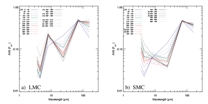
Figure 7.— Average normalized radial IR SEDs for the –a) LMC and –b) SMC. Each line represents the average of the normalized (by TIR) fluxes of all of the Hii regions in an annulus with inner and outer radii (labeled in the upper left). The parenthetical numbers to the left of the labels correspond to the number of Hii regions included for each annulus. The colors of the lines go from the inner annuli (blue), to middle annuli (green and red), and finally to the outer annuli (black and gray).

The normalized 8 $\mu$m aromatic emission behaves very differently in the LMC than in the SMC. In the LMC the average $F_{\mbox{\tiny{N}}},_{8}$ values increase slightly with radius. In the SMC the average $F_{\mbox{\tiny{N}}},_{8}$ values do not follow an obvious trend with radius. The 8 $\mu$m emission in the SMC Hii regions on average accounts for about $7\%$ of their TIR, while in the LMC Hii regions, aromatics account for $15\%$ of the TIR. The lower normalized 8 $\mu$m values in the SMC are at least partially due to the lower intrinsic fluxes at 8 $\mu$m for SMC Hii regions, and the SMC in general (see Figure 5). The lack of a radial trend for the 8 $\mu$m emission in the SMC may be a combination of the lack of aromatics, in which we would expect a trend similar to the LMC 8 $\mu$m where aromatics emission increases away from the central ionizing source, and potential contributions to the 8 $\mu$m from other bands. For instance, the [Arii] nebular emission line is not expected to contribute much to the 8 $\mu$m emission (Lebouteiller et al., 2007), but the lack of strong aromatics in the SMC means that this weaker line, along with Hi and [Ariii] emission (Peeters et al., 2002; Lebouteiller et al., 2007), may be more significant factors in the observed 8 $\mu$m fluxes. The contribution of non-aromatic emission to the 8 $\mu$m fluxes within SMC Hii regions needs to be more fully explored. The lower SMC 8 $\mu$m emission is further discussed in section 6.3.

The $F_{\mbox{\tiny{N}}},_{70}$ values are nearly constant among all annuli for both the LMC and SMC ($70~{}\mu\mbox{m}\approx 45\%$ TIR). Thus, the SEDs in each annuli must all peak near 70 $\mu$m and the peak of the SED must not considerably vary as we spatially observe the Hii regions from their centers outward. We further explore the implications of this result in the following sections.

6.2. Physical Sizes of Hii Region Complexes

The appropriate size aperture to use for extragalactic studies of Hii regions is unknown and is typically set by the limiting resolution of the instrument because many of the Hii regions are not resolved in the IR at extragalactic distances. An incorrect aperture size will add uncertainties to any SFR calculation because the accumulated flux may not all be from the Hii region of interest. We explore the Hii complex size scales, as probed by the 8, 24, 70, and 160 $\mu$m dust emission, and compare them to the size scales found using the TIR flux.

We quantitatively probe the sizes of the LMC and SMC Hii regions by tracing the TIR, 8, 24, 70, and 160 $\mu$m radial profiles (see Figure 6) and calculate the radius at which each band’s surface brightness drops by $95\%$ ($\sim 2\sigma$) from that measured in the inner $35\arcsec$ ($\sim 10$ pc) radius aperture. All four dust bands peak in the center aperture for every Hii region (see Figure 6), and the central aperture is where we are most certain that young stars dominate the UV output.

The results of our size determinations can be found in Table 3. The size for each LMC and SMC Hii region complex is listed along with the radius in arcseconds where the surface brightness drops to less than $5\%$ of the surface brightness of the inner aperture. The mean, standard deviation, and fractional error (standard deviation divided by the mean) for the LMC and SMC Hii complexes are also tabulated. The Hii region sizes have large standard deviations about the mean values. The errors, as a fraction of the mean, are $31\%-39\%$ for all bands.

Table 3Sizes of Hii Region Complexes

	TIR	$8\mu$m	$24\mu$m	$70\mu$m	$160\mu$m
Name	Radius (arcsec)
LMC
N4	140	210	105	140	210
N11	245	490	210	245	420
N30	210	280	140	210	350
N44	315	385	210	315	350
N48	315	385	140	315	420
N55	245	245	210	245	245
N59	175	245	140	175	245
N79	140	175	105	140	210
N105	175	210	140	175	245
N119	385	490	280	420	490
N144	210	280	175	210	315
N157	NAa	280	NAa	315	NAa
N160	175	245	140	210	490
N180	315	490	245	315	490
N191	140	140	105	140	140
N206	315	350	210	315	385
Mean	233	306	170	243	334
Std dev	79	113	54	82	114
Fr.errorc	0.34	0.37	0.32	0.34	0.34
SMC
DEM74	NAb	NAb	245	NAb	NAb
N13	245	210	140	245	350
N17	280	280	210	280	315
N19	280	280	245	280	315
N22	245	245	140	245	315
N36	455	385	385	455	490
N50	525	490	315	525	560
N51	280	245	140	280	350
N63	210	245	210	210	210
N66	210	210	175	245	280
N71	140	280	140	140	210
N76	315	NAb	245	315	NAb
N78	140	140	105	140	210
N80	350	280	210	315	385
N84	315	280	210	315	350
N90	175	210	140	175	210
Mean	278	270	203	278	325
Std dev	107	84	74	105	105
Fr.errorc	0.39	0.31	0.36	0.38	0.32

Note. — Hii complex sizes are computed using the method described in section 6.2.

For the TIR in the LMC Hii regions, the minimum/maximum radii measured are 140/385 arcsec (35/97 pc), respectively. For the TIR in the SMC Hii regions, the minimum/maximum radii measured are 140/525 arcsec (41/154 pc), respectively. The computed sizes listed in Table 3 are not drastically different for the LMC and the SMC, particularly given the large standard deviations.

The sizes calculated from TIR, though not identical, are close to the sizes calculated using the 70 $\mu$m emission. This can most clearly be seen in Figure 8 where we plot the Hii region 8, 24, 70, and 160 $\mu$m sizes, normalized by the TIR sizes. The mean $F_{\mbox{\tiny{N}}},_{70}$ size falls nearly on the vertical dotted line associated with TIR for both the LMC and SMC. The standard deviation in the sizes measured using $F_{\mbox{\tiny{N}}},_{70}$ is smaller than for the sizes measured using the other normalized bands. This is a another consequence of 70 $\mu$m being near the peak of dust SED (see Section 6.1). The mean size of the Hii regions using either TIR or 70 $\mu$m is $60\pm 20$ pc the LMC and $80\pm 30$ pc for the SMC.

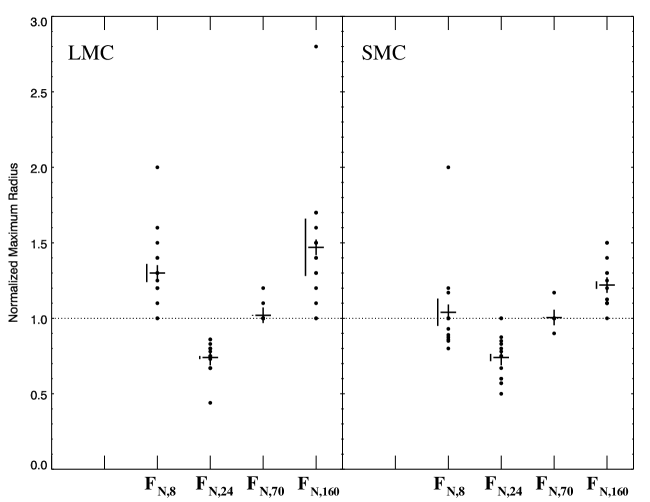
Figure 8.— LMC and SMC Hii region sizes of the 8, 24, 70, and 160 $\mu$m fluxes normalized by the sizes computed using TIR. The LMC is plotted in the left panel, and the SMC is plotted in the right panel. The points are the data, the crosses are the mean values, and the solid lines to the left of the data are the $\pm 1\sigma$ standard deviations. All of the Hii regions in Table 3 are included, but many of the individual Hii regions overlap due to discrete $35\arcsec$ increasing radii for successive annuli. The horizontal dotted line marks the positions where the sizes of the monochromatic bands are equal to the computed sizes measured using TIR.

The calculated 8 $\mu$m sizes in the LMC are as large as or larger than sizes measured using 70 $\mu$m or TIR, with the exception of 30 Doradus (N157). There is no such trend in the SMC where the sizes traced by the 8 $\mu$m emission may be larger or smaller than the sizes calculated using the 70 $\mu$m dust emission. This is shown in Figure 8 where the sizes of the Hii regions, as measured by $F_{\mbox{\tiny{N}}},_{8}$, are systematically larger than TIR in the LMC but roughly scattered around TIR in the SMC. This trend is consistent with the 8 $\mu$m flux following a shallower decline with radius in the LMC relative to the SMC. The mean size of the Hii regions using 8 $\mu$m is $75\pm 35$ pc for the LMC and $80\pm 25$ pc for the SMC.

All of the Hii regions are smallest when calculated using the 24 $\mu$m emission. This is consistent with others who have found the warm small dust grains probed by 24 $\mu$m being more heavily peaked near the center of star forming regions (e.g., Relaño & Kennicutt, 2009). None of the Hii regions have sizes measured via $F_{\mbox{\tiny{N}}},_{24}$ in Figure 8 that are larger than the sizes calculated via TIR. The mean size of the Hii regions using 24 $\mu$m is $40\pm 15$ pc for the LMC and $60\pm 20$ pc for the SMC.

The mean size of the Hii regions using 160 $\mu$m is $85\pm 30$ pc for the LMC and $95\pm 30$ pc for the SMC. We have shown in Figure 7 that the $F_{\mbox{\tiny{N}}},_{160}$ averages in the Hii region SEDs are largest at large radii (also discussed in section 6.3). Consequently, the Hii region sizes, as probed by 160 $\mu$m emission, are generally larger than the sizes calculated using the other IR dust bands. When the sizes measured via the TIR and 160 $\mu$m emission are compared (see Figure 8), the sizes calculated using the cold 160 $\mu$m emitting dust are systematically larger or the same size as the TIR in both the LMC and SMC. The sizes measured by the cold dust emission at 160 $\mu$m are the largest despite the fact that the 160 $\mu$m surface brightnesses peak in the center of the Hii regions (see Figure 6). The increasing importance of the 160 $\mu$m emission to the TIR in the outer radii of the Hii regions causes a relatively shallow decline in flux with radius. The computed large Hii region cold dust sizes are a consequence of the pervasiveness of the cold dust emission to large radii.

From this analysis, we conclude that the sizes of Hii regions, as probed by dust, depend greatly on the wavelength observed but also depend greatly on the individual Hii region due to the large deviations in each band. The warmer dust probed by 24 $\mu$m will give smaller Hii region sizes than the cold dust probed by 160 $\mu$m. The sizes probed by 70 $\mu$m emission is nearly identical to the sizes probed by the TIR, with little scatter. This is a consequence of the IR SEDs peaking near 70 $\mu$m at all spatial distances for nearly every Hii region (see section 6.1). Thus, when taking into account the limits of resolution and aperture size for extragalactic studies, 70 $\mu$m is the most ideal of the monochromatic IR star formation indicators because it will trace the TIR spatially and extend to physically larger distances than, say, the 24 $\mu$m emission. Furthermore, we show in Figure 8$a$ that for most of the Hii regions in our sample, an aperture radius of $\sim 100$ pc would be adequate for acquiring most of the 70 $\mu$m flux.

The size distribution of the nebular portion of Hii regions, as traced by H$\alpha$, has been extensively studied and argued to follow either a power law (Kennicutt & Hodge, 1980) or an exponential law (van den Bergh, 1981). Given that the luminosity function is calculated to follow a power law, Oey et al. (2003) argue that the size distribution must also follow a power law because the luminosity measurements come from ionizing photons within a specific nebular volume. For the Magellanic Clouds, Kennicutt & Hodge (1986) use an exponential function to estimate the scale length for Hii region sizes to be $\sim 80$ pc. From our data, we cannot determine a statistically significant size distribution for the LMC or SMC because our sample is too small. The initial selection of our 32 Hii regions was by eye which will bias any size distributions created from this data. A more objective IR selection of a larger number of LMC and SMC Hii regions is required for an analysis of the LMC and SMC Hii region size distributions, particularly at the small end. Ignoring the warmer dust probed via 24 $\mu$m, the sizes we do measure are roughly the same as that of the Kennicutt & Hodge (1986) derived H$\alpha$ size distribution scale length.

It must be stated that the sizes we measure include the general star forming regions. The dust emission is high out to relatively large distances. Our size estimates are not directly comparable to the H$\alpha$-derived nebular sizes. Although there may be similarities in that the IR-measured sizes of the LMC Hii regions should be somewhat larger than those in the SMC because the H$\alpha$ and IRAS 100 $\mu$m luminosity functions in the LMC have a higher mass cut-off than in the SMC (see discussion in Section 5.1; Kennicutt & Hodge, 1986; Livanou et al., 2007). The large standard deviations of the IR-derived sizes is real because the scatter in the surface brightness profiles from which they are derived is real (see section 5.3). This scatter is probably introduced by sampling Hii regions of different high mass stellar populations and evolutionary histories, which are two components that shape the H$\alpha$ luminosity function (Oey & Clarke, 1998).

6.3. TIR Normalized Radial Profiles

Plotted in Figure 9 are the 8, 24, 70, and 160 $\mu$m radial profiles, normalized by TIR, ($F_{\mbox{\tiny{N}}},_{\nu}$), of the LMC and SMC Hii regions. For the LMC Hii regions, the $F_{\mbox{\tiny{N}}},_{8}$ emission is truncated near the center of the Hii regions (down to $\sim 10\%$ TIR) and is relatively constant ($\sim 20\%-25\%$ TIR) for annuli with radii greater than $\sim 200\arcsec$ ($\sim 50$ pc). The $F_{\mbox{\tiny{N}}},_{24}$ emission is sharply peaked near the centers of the Hii regions ($\sim 20\%$ TIR) and falls to a modest level ($\sim 5\%-10\%$ TIR) for annuli with radii greater than $\sim 200\arcsec$ ($\sim 50$ pc). The $F_{\mbox{\tiny{N}}},_{70}$ emission is relatively constant for all radii probed here ($\sim 40\%-50\%$ TIR). The $F_{\mbox{\tiny{N}}},_{160}$ emission increases dramatically with aperture/annuli radii, from ($\sim 20\%$ TIR) near the core to ($\sim 50\%$ TIR) near the outer annuli. The scatter about the mean for $F_{\mbox{\tiny{N}}},_{160}$ is larger than for the other emission bands. The 8 $\mu$m outliers in Figure 9$a$ are from the N4 Hii region, where two bright 8 $\mu$m sources are included in the outer annuli at $\sim 260$ pc from the center (see N4 in Figure 3).

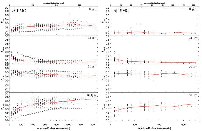
Figure 9.— Radial profiles, from top to bottom, of the 8, 24, 70, and 160 $\mu$m fluxes, normalized by TIR, for the –a) 16 LMC Hii regions and –b) 16 SMC Hii regions. The $\pm 1\sigma$ statistical errors are on the order of the point sizes. The red line traces the average normalized flux, calculated for each annulus. Spatial units (parsecs) are labeled on the top axis. The boxes in panel (a) represent 30 Doradus (N157) and are not included in the average value (red line) because 30 Doradus is saturated around the core in 24 and 160 $\mu$m.

For the SMC Hii regions, the $F_{\mbox{\tiny{N}}},_{8}$ does not show an increase from the central core as it does in the LMC. The $F_{\mbox{\tiny{N}}},_{8}$ is consistently around $5\%$ TIR at all radii, which is significantly smaller than in the LMC. The $F_{\mbox{\tiny{N}}},_{24}$ emission is peaked in the center as it is for the LMC, although to a smaller magnitude ($\sim 15\%$ TIR). The $F_{\mbox{\tiny{N}}},_{70}$ emission in the SMC is consistent with that for the LMC, at all annuli radii. The $F_{\mbox{\tiny{N}}},_{160}$ emission is also similar to that for the LMC.

Due to the change in the shape of the $F_{\mbox{\tiny{N}}},_{24}$ profile at low radii, 24 $\mu$m may not be as robust a tracer of TIR (or obscured SFR) as 70 $\mu$m, which has a relatively constant profile with radius. An observer would need to develop a conversion from 24 $\mu$m to TIR that is dependent on the radius of the aperture used for the measurement.

The average SMC $F_{\mbox{\tiny{N}}},_{8}$ profile in Figure 9 is depressed relative to the LMC at all scales. The same is true, although to a lesser extent, for the $F_{\mbox{\tiny{N}}},_{24}$ profile. The 8 and 24 $\mu$m fluxes are at least partially associated with aromatics/small grains undergoing stochastic heating (Puget & Leger, 1989; Draine & Li, 2007). The low values of $F_{\mbox{\tiny{N}}},_{8}$ and $F_{\mbox{\tiny{N}}},_{24}$ in the SMC relative to the LMC are an indication that the SMC has fewer of these aromatics/small grains. This is consistent with the results in K. D. Gordon et al. (2010, in preparation) who find that the SMC has an aromatic fraction of $1.1\%$, which puts the aromatic abundance in the SMC on the low end of the Draine et al. (2007) Spitzer SINGS sample. This is also consistent with the SMC’s low metallicity and high radiation field hardness (Gordon et al., 2008). The strong dependence of the host galaxy’s aromatic/small grain population presents a problem for using either of these bands as a monochromatic star formation indicator. Previous works have noted some of these potential problems when using 8 or 24 $\mu$m as star formation indicators (e.g., Dale et al., 2005; Calzetti et al., 2005, 2007).

In Figure 10, we show the fractional error ($1\sigma/\mbox{mean}$) of the $F_{\mbox{\tiny{N}}},_{\nu}$ measurements for each annulus. Plotted are the fractional errors with respect to annuli radius for the LMC (panel a) and SMC (panel b). For all radii, except for perhaps at the largest radii measured here where low number statistics dominate, the fractional error of the $F_{\mbox{\tiny{N}}},_{70}$ indicator is lower than the other IR dust emission bands and is $\sim 5\%-12\%$ the mean value at radii less than 240 pc in the LMC and SMC. The fractional error of $F_{\mbox{\tiny{N}}},_{24}$ is $>0.15$ until the largest radii where low number statistics become an issue.

Figure 10.— Fractional errors ($\sigma$/mean) of the 8 (open squares), 24 (open diamonds), 70 (filled circles), and 160 $\mu$m (open triangles) TIR normalized radial profiles for the –a) LMC and –b) SMC. Physical spatial units (parsecs) are given on the top axis. Due to saturation in 24 and 160 $\mu$m, the 30 Doradus (N157) Hii region is not included in the LMC computations of fractional errors

Using the IR fluxes, normalized by the TIR, we find that the 70 $\mu$m emission is a robust tracer of the TIR, and thus the star formation obscured by dust. This is because the normalized 70 $\mu$m flux is relatively constant (70 $\mu\mbox{m}\sim 0.40-0.50~{}\mbox{TIR}$) for all radii measured, does not systematically vary between the LMC and SMC, and has the smallest fractional errors at nearly every radii. These results are consequences of the fact that the SEDs of the Hii region annuli in our sample all peak near $70~{}\mu$m (see section 6.1).

These results will be less robust for galaxies that have Hii regions that are hotter than the typical LMC or SMC Hii region. However, we do not expect this to be the case because the hottest Hii region in our sample, 30 Doradus, would fall on the high end of any Hii region H$\alpha$-derived luminosity function (Kennicutt et al., 1989). If hotter Hii regions are more common in a particular galaxy, they will have dust profiles more like 30 Doradus (see boxes in Figure 9$a$) where the 24 $\mu$m flux is a larger percentage of the TIR out to larger radii. Consequently, the normalized 70 $\mu$m flux is reduced near the core. This produces an increasing slope in $F_{\mbox{\tiny{N}}},_{70}$ until some radius where the 24 $\mu$m emission is no longer a dominant contributor to the TIR. It is probable that we would see this effect on smaller scales than is probed in this work for all Hii regions.

The photons of hotter Hii regions will also affect the observed 8 and 160 $\mu$m normalized fluxes. The hotter Hii regions may push the photoionization front to larger radii causing a decrement of aromatics near the core. Thus, the peak normalized 8 $\mu$m flux would occur at larger radii. The 160 $\mu$m flux would not dominate the TIR until even larger radii than is measured in this work. If hotter Hii regions are more common in other galaxies, then there will be a larger scatter about the average $F_{\mbox{\tiny{N}}},_{70}$ ratio with larger variations near the core.

6.4. Star Formation Rates

6.4.1 Radial SFR Densities

For the star formation obscured by dust, we use the TIR SFR computation from Equation (4) of Kennicutt (1998). The Kennicutt (1998) obscured SFR equation is valid for starbursts, but dust emission in Hii regions and starburst galaxies of varying metallicities and ionization measures behave similarly (Gordon et al., 2008; Engelbracht et al., 2008). Dust obscured star formation in Hii regions is similar to star formation in starbursts because starbursts are usually very dusty and, furthermore, were likely the birthplaces of most of the present-day stars (Elbaz & Cesarsky, 2003; Bernard-Salas et al., 2009). The Kennicutt (1998) obscured SFR equation takes the form of

$$\mbox{SFR}=4.5\times 10^{-44}~{}L_{TIR},$$ (3)

where SFR is the star formation rate in units of solar masses per year. The value $4.5\times 10^{-44}$ is a constant derived from spectral synthesis models, assumptions on the shape of the initial mass function (IMF), and assumptions on the timescale of the star formation event (Kennicutt, 1998). $L_{TIR}$ is the TIR luminosity in units of ergs per second. Similarly, we use Equations 1 and 2 in Kennicutt (1998) to calculate the unobscured SFRs derived from UV and H$\alpha$, which rely on similar assumptions. In all three cases a Salpeter IMF is assumed (Salpeter, 1955).

It is noted by Relaño & Kennicutt (2009) and Helou et al. (2004) that H$\alpha$ emission peaks near the maximum 24 $\mu$m emission. However, the peak UV emission is offset from H$\alpha$ and 24 $\mu$m, presumably because the UV emission is absorbed by the dust where the H$\alpha$ and 24 $\mu$m emit the strongest (Relaño & Kennicutt, 2009). We also find that H$\alpha$ peaks near the peak 24 $\mu$m emission (see Figures 1 and 2). The UV fluxes in the LMC data indicate a peak UV emission near the peak H$\alpha$ and 24 $\mu$m fluxes, but as a result of our spatial resolution we cannot determine if the UV is offset from the peak H$\alpha$ or 24 $\mu$m emission as is claimed by Relaño & Kennicutt (2009). There are regions in the LMC with strong UV fluxes but weak or absent H$\alpha$ and 24 $\mu$m fluxes. Many of these UV fluxes are found in the centers of noted Hi supergiant shells where hot OB stars and supernovae remnants have cleared out much of the gas and dust and triggered star formation on their peripheries (see Kim et al., 1999; Cohen et al., 2003).

In Figure 11, we show the radial dependence of SFR densities ($M_{\odot}$ yr^-1 pc^-2) derived using the obscured SFR indicator (TIR) and the unobscured SFR indicator (H$\alpha$) for the LMC (panel a) and the SMC (panel b). The magnitudes of the SFR densities depend on the aforementioned assumptions about the IMF, star formation timescales, and spectral synthesis models used (Kennicutt, 1998). However, the magnitudes are not crucial for this analysis. It is only the dependence with radius that we wish to convey. The general trends of the obscured and unobscured SFRs with radius will be constant because all conversions from a star formation indicator to a SFR depend upon a constant value.

Figure 11.— Computed radial obscured (TIR–top panels) and unobscured (H$\alpha$–middle panels) SFR densities ($M_{\odot}$ yr^-1 pc^-2) for each of the –a) LMC and –b) SMC Hii regions, using the SFR equations 2 and 4 from Kennicutt (1998). The bottom panels are the ratio of the obscured TIR-derived SFRs to the unobscured H$\alpha$-derived SFRs. The radial units are in arcseconds with spatial radial units of parsecs on the top axis.

The obscured and unobscured SFR densities in the LMC are larger than in the SMC, which is expected given the larger LMC Hii region luminosities (see Section 5.1) and the high-end cutoff at larger luminosities for the LMC H$\alpha$ and IR luminosity functions (Kennicutt & Hodge, 1986; Livanou et al., 2007).

For the obscured SFR densities, both the LMC and SMC show a peak in the inner annuli and a decrease outward. This is expected given that the TIR emission peaks in the centers of the Hii regions as plotted in Figure 6. The unobscured SFR densities, calculated via H$\alpha$, also peak in the center for LMC Hii regions. Because the 24 $\mu$m emission peaks where the TIR emission peaks in Figure 6, these results are further evidence, along with the results in Figure 1, that the 24 $\mu$m emission traces the H$\alpha$ emission. Along the same lines, the 8, 70, and 160 $\mu$m peak fluxes will also trace the peak H$\alpha$ fluxes. These results should break down on smaller scales than measured here because the dust grains may be destroyed when near the central ionizing stars. For example, it is noted that the aromatics probed with 8 $\mu$m are not observed to be any nearer the central OB stars than in the outlying PDRs (Relaño & Kennicutt, 2009; Snider et al., 2009; Watson et al., 2008; Helou et al., 2004).

The H$\alpha$-derived unobscured SFR densities are slightly offset from the TIR-derived obscured SFR densities in the SMC (see middle panel of Figure 11). There is a slight decline of the H$\alpha$ determined unobscured SFR densities in the inner aperture. This may well be a consequence of our limited H$\alpha$ resolution. We aim to explore this in the future with higher resolution data.

As shown in the bottom panel of Figure 11$a$, the ratios of obscured SFR densities to the unobscured SFR densities slightly increase with radius in the LMC. If this trend is real then it indicates that H$\alpha$ is more strongly peaked in the center of an Hii region than TIR. One possible explanation is that the TIR is a measurement that includes dust at many temperatures. As shown earlier, the colder dust dominates at larger radii. This trend is not seen in the SMC, although, we do not trace many of the SMC Hii regions out to large radii.

We do not have UV data of the SMC, but we do have UV data of the LMC. For the LMC, we can do the same analysis of unobscured SFRs via UV as we did with H$\alpha$ (see Figure 12). In general, the UV-derived SFR densities are similar to the TIR-derived SFR densities in that they are both centrally peaked. The spatial congruence is probably a resolution effect because it is contrary to the higher resolution work of (Relaño & Kennicutt, 2009) who found UV emission offset from IR emission. There is no discernable trend in the ratio of obscured to unobscured SFRs in the bottom panel.

Figure 12.— Computed radial obscured (TIR–top panel) and unobscured (UV–middle panel) SFR densities ($M_{\odot}$ yr^-1 pc^-2) for the LMC Hii regions, using the SFR equations 1 and 4 from Kennicutt (1998). The bottom panel is the ratio of the obscured TIR-derived SFRs to the unobscured UV-derived SFRs. The radial units are in arcseconds with spatial radial units of parsecs on the top axis.

6.4.2 Obscured SFR Indicators

It is well argued that the TIR is the best obscured SFR indicator (Kennicutt, 1998), and, indeed, Kennicutt et al. (2009) find that TIR is a better star formation indicator than 8 or 24 $\mu$m. However, if an observer does not have multiple IR bands then it may be difficult to make an accurate calculation of TIR. Thus, a monochromatic star formation indicator that can reliably recover the TIR over a large spatial scale is valuable.

We substitute the TIR luminosity in Equation 3 with the 8, 24, 70, and 160 $\mu$m luminosities by using the average luminosity of a given band, normalized by TIR. The resulting SFR equation contains observable quantities. These equations take the same form as Eq. 3, but there are band specific constants added ($C_{8}$, $C_{24}$, $C_{70}$, and $C_{160}$) that are from the factor $L_{\nu}L_{TIR}^{-1}$ used to transform $L_{TIR}$ to $L_{\nu}$. From these constants we compute the SFRs ($M_{\odot}$ yr^-1) using the measured 8, 24, 70, or 160 $\mu$m luminosities (ergs s^-1),

$$\mbox{SFR}=4.5\times 10^{-44}~{}C_{\nu}~{}L_{\nu},$$ (4)

where SFR is in units of solar mass per year, $4.5\times 10^{-44}$ is the constant from Kennicutt (1998), $C_{\nu}$ is the IR band specific constant, and $L_{\nu}$ is the observed luminosity in ergs per second.

In Table 4, we show the aperture size-dependent constants used for the aperture radial sizes from 10 to 300 pc for the LMC (top rows) and from 10 to 200 pc for the SMC (bottom rows). Listed in the columns are the size of the aperture radius in parsecs, the SFR equation constants, and the number of Hii regions included in the calculation. 30 Doradus was not included in these calculations due to the saturation of 24 and 160 $\mu$m.

Table 4SFR Equation Average Constants

Radius	$C_{8}$	$C_{24}$	$C_{70}$	$C_{160}$	$N$
(pca)
LMC
10	$8.84\pm 1.80$	$5.07\pm 0.80$	$2.19\pm 0.15$	$6.11\pm 2.40$	15
20	$8.30\pm 1.79$	$5.89\pm 0.91$	$2.10\pm 0.11$	$5.42\pm 1.70$	15
50	$6.65\pm 1.22$	$7.92\pm 1.43$	$2.08\pm 0.12$	$4.05\pm 0.93$	15
100	$5.79\pm 0.97$	$9.85\pm 1.98$	$2.11\pm 0.15$	$3.39\pm 0.74$	15
200	$5.09\pm 0.83$	$12.46\pm 2.46$	$2.18\pm 0.17$	$2.83\pm 0.65$	13
300	$4.57\pm 0.27$	$14.36\pm 2.16$	$2.23\pm 0.11$	$2.49\pm 0.32$	4
SMC
10	$16.64\pm 3.14$	$8.72\pm 3.33$	$2.22\pm 0.18$	$4.46\pm 1.62$	16
20	$16.45\pm 3.26$	$10.16\pm 3.45$	$2.18\pm 0.15$	$4.09\pm 1.32$	16
50	$16.70\pm 4.40$	$13.55\pm 4.75$	$2.17\pm 0.15$	$3.53\pm 0.87$	16
100	$16.49\pm 5.45$	$16.33\pm 5.63$	$2.19\pm 0.15$	$3.20\pm 0.63$	16
200	$18.82\pm 3.18$	$11.93\pm 4.61$	$2.18\pm 0.19$	$3.49\pm 1.05$	2

Note. — Constants to the SFR equations are calculated for each aperture radius (parsecs). The top values are for the LMC and the bottom values are for the SMC. The constants are defined in Section 6.4.2. 30 Doradus (N157) has been removed from this analysis due to saturation in the core in 24 and 160 $\mu$m. The uncertainties are given as $\pm 1\sigma$.

The SFR equations for each of the observable bands are dependent on the physical scale of the instrumental PSF, particularly for the 8, 24, and 160 $\mu$m luminosities. The deviation of 8 and 24 $\mu$m between the LMC and SMC, as discussed in section 6.3, can be seen in the differences of $C_{8}$ and $C_{24}$ in Table 4. The 70 $\mu$m band specific constants, $C_{70}$, do not vary between the LMC and SMC, or with radius, within the $\pm 1\sigma$ standard deviations. Any SFRs derived from the 8, 24, or 160 $\mu$m luminosities should be used with caution.

The Calzetti et al. (2007) SFR formalism is commonly used in the literature (e.g., Wu et al., 2008; Galametz et al., 2009). Using 24 $\mu$m, we compare the SFRs calculated from our Kennicutt (1998) modified method with the extinction-corrected method of Calzetti et al. (2007, see their Equation (9)) for apertures of increasing size. The SFR equation in Calzetti et al. (2007) is computed by finding a best-fit line through a plot of Pa$\alpha$ luminosity versus 24 $\mu$m luminosity, but using the highest metallicity galaxies in their sample. In the inner radii ($\sim 10$ pc) of our sample, the results using the formalism of Calzetti et al. (2007) produce SFRs that are greater by a factor of 2 in the LMC and 1.7 in the SMC. The SFRs between the two methods slowly equilibrate with radius until they are nearly identical at a radius of $\sim 280$ pc in the LMC and $\sim 140$ pc in the SMC. The results diverge again in the outskirts of the Hii regions. At 200 pc, the Calzetti et al. (2007) method produces SFRs that are $\sim 2/3$ the value of our SFRs in the LMC and $\sim 3/4$ the value of our SFRs in the SMC. It is reasonable to expect our SFRs to be lower near the center of Hii regions because we do not take into account the unextincted UV photons that is in the Calzetti et al. (2007) formalism. The LMC and SMC differences are likely because the formalism of Calzetti et al. (2007) assumes high metallicity systems, whereas, the LMC and SMC have different, and low, metallicities. Thus, the SFR formalism of Calzetti et al. (2007) is not as accurate for lower metallicity systems, but our derived SFR formalism is less accurate if there is a large percentage of unextincted UV photons. Thus, we stress that our star formation formalism provides obscured SFRs.

Wu et al. (2008) also use 24 $\mu$m as a star formation indicator. They do a study of 28 compact dwarf galaxies and calculate SFRs using the 24 $\mu$m SFR recipe from Wu et al. (2005), which was derived using the observed correlations between H$\alpha$, 1.4 GHz, and 24 $\mu$m luminosities. Unlike the Calzetti et al. (2007) sample, Wu et al. (2005) include both metal-poor and metal-rich galaxies. The SFRs used via the Wu et al. (2005) method better match the SFRs estimated using 1.4 GHz, and Wu et al. (2008) note that this method derives SFRs that are up to several times larger than the SFRs derived using the formalism from Calzetti et al. (2007). Comparing our Kennicutt (1998) modified 24 $\mu$m method of calculating radial cumulative SFRs with the results of Calzetti et al. (2007) and Wu et al. (2005), we find that the SFRs measured using our method are $\sim 35\%-57\%$ the values found using the Wu et al. (2005) method, for all radii. This differs from the results of Calzetti et al. (2007), where our SFRs became relatively greater at larger radii. Thus, SFRs calculated at larger radii using our formalism lie between those giving higher SFRs using the Wu et al. (2005) method and the lower SFRs calculated using the Calzetti et al. (2007) method. These results are consistent because the LMC and SMC have lower metallicities than the normal star forming galaxies used to derive the Calzetti et al. (2007) formalism.

By observing 22 starburst galaxies, Brandl et al. (2006) explore the use of aromatics as star formation indicators. They find a correlation between the aromatic 6.2 $\mu$m emission and the TIR, where the TIR calculated is uncertain to within a factor of 2. Using our measured aromatic 8 $\mu$m emission and the uncertainties in $C_{8}$ in Table 4, we can derive TIRs that are uncertain by a factor of $\sim 1.2-1.5$ in the LMC and $\sim 1.2-2.0$ in the SMC. The differences in our uncertainties are due to the changing dispersions of $C_{8}$ between the LMC and SMC and between radii. The SMC correlations are more uncertain in our sample than the LMC correlations. Our results are comparable or better than the results of Brandl et al. (2006). Our measurements do not suffer as much from the introduction of diffuse dust emission because we center our observations around star forming areas. The Brandl et al. (2006) dataset uses the Spitzer IRS slits, and the smallest linear scales they probe are about 200 pc, whereas, we probe down to $\approx 20$ pc. Brandl et al. (2006) note that any local variations may be “averaged out” in their measurements.

The results of Brandl et al. (2006) illustrate some of the difficulties in estimating TIR associated with star formation when averaging over an entire galaxy. Our data are acquired by observing around the central ionizing sources of the Hii regions. Thus, a caveat is that our results are more applicable to star forming regions and not entire galaxies, where the IR emission of cold diffuse dust is more prominent. As an example, the average $C_{70}$ value for the LMC and SMC is 2.17, which corresponds to $L_{TIR}=0.46\times L_{70}$. The derived values of $C_{70}$ using the total LMC and SMC galactic apertures are 2.56 and 2.22, respectively. The SMC value is on the high end measured in Table 4, and the total LMC $C_{70}$ constant is larger, beyond the $\pm 1\sigma$ standard deviations, of those measured for the average Hii regions at any radii in Table 4. The uncertainty on the final calculated SFR after integrating over an entire galaxy will depend upon how much of the IR photons originate from star forming regions and how much are due to photons from the general stellar population.

6.4.3 The 70 $\mu$m Star Formation Proxy

The results in Table 4 indicate that 70 $\mu$m is the most suitable obscured SFR indicator. The $C_{70}$ constant remains the same value for all radii and between the LMC and SMC, within the $1\sigma$ standard deviations. For these reasons, we calculate one mean value of $C_{70}$ using all of the $C_{70}$ values at every radius from 10 to 300 pc, including both the LMC and SMC. From this, we have computed a monochromatic 70 $\mu$m SFR equation using the formalism from Equation (4) of Kennicutt (1998) and the mean value of $C_{70}$. The monochromatic obscured SFR equation is

$$\mbox{SFR}=9.7(0.7)\times 10^{-44}~{}L_{70},$$ (5)

where SFR is in units of solar masses per year and $L_{70}$ is in units of ergs per second. The $1\sigma$ standard deviation in Equation (5) is from the uncertainties in the spread of $C_{70}$. The mean of the $C_{70}$ radial averages is $2.17$ and the 1 $\sigma$ standard deviation (0.15) comes from the mean of the $C_{70}$ radial standard deviations. The $1\sigma$ standard deviation of $C_{70}$ is only $\sim 7\%$ of the mean value of $C_{70}$. As is the case for the original obscured SFR equation from Kennicutt (1998) (see Eq. 3), this equation works as a good approximation for the total SFR if the area measured is almost entirely obscured by dust.

We calculate the total obscured SFR of the LMC, using Equation 5 and the cumulative 70 $\mu$m flux of the LMC (see section 5.1). The LMC obscured SFR of 0.17 ($M_{\odot}$ yr^-1) agrees well with the results of Harris & Zaritsky (2009) who estimate the total mean LMC SFR to be 0.2 ($M_{\odot}$ yr^-1), with variations over the last five billion years of up to a factor of two.

The usefulness of Equation (5) extends to Hii regions measured with aperture radii anywhere from 10 to 300 pc. Care should be taken if measuring sizes outside of these ranges. On very small physical scales our relation, as all others, should break down because the effects of individual protostars and stars will become important (Indebetouw et al., 2008). Furthermore, the effects of hotter Hii regions, like 30 Doradus, may result in a radially dependent 70/TIR ratio that would introduce errors into our formalism at lower radii (see the discussion in section 6.3). There is also the possibility that the luminosities of smaller Hii regions are different than expected from a presumed IMF due to small number statistics (Oey & Clarke, 1998). For the same reason, Indebetouw et al. (2008) argue that measurements of many smaller clusters will produce SFRs that are too low since they are not fully sampling the stellar IMF.

Equation (5) also may not hold at very large radial distances because of dust emission excited from older (colder) stellar populations contaminating the IR SEDs. Further work must be done to model the contribution of older stellar populations to the 70 $\mu$m emission, particularly in the outer regions. A careful background subtraction will help mitigate any contamination, and a modest annulus of radius $\sim 100$ pc is all that is required to obtain most of the bolometric dust emission in the LMC and SMC Hii regions (see section 6.2). Furthermore, our equation is valid over the wide range of Hii region luminosities and sizes probed in this work. The low end of the Magellanic Cloud luminosity functions includes clusters with luminosities on the order of the Orion Nebula (Kennicutt & Hodge, 1986), approximately equivalent to N90 in the SMC, while the high end covers the massive 30 Doradus Hii region. However, this research would benefit from a sample of Hii regions in a larger galaxy sample so as to more broadly explore environmental effects.

7. CONCLUSIONS

We performed UV, H$\alpha$, and IR aperture/annulus photometry of 16 LMC and 16 SMC Hii regions at the common resolution of the MIPS 160 $\mu$m $40\arcsec$ FWHM PSF. With the aperture photometry, we computed IR SEDs using the total cumulative Spitzer IRAC (3.6, 4.5, 8 $\mu$m) and MIPS (24, 70, 160 $\mu$m) fluxes of the LMC, SMC, and each Hii region. The cumulative SED of the LMC is brighter than the SMC, and their shapes are consistent with IR SEDs of the Magellanic Clouds in the literature. The SMC Hii regions have cumulative fluxes that are weaker, by about an order of magnitude, than the LMC Hii regions. We argue that this is expected from what is known about the LMC and SMC Hii region luminosity functions.

We compute the IR bolometric flux (TIR) for each Hii region aperture/annulus by integrating under the linear extrapolation of the 8, 24, 70, and 160 $\mu$m fluxes. We include the input from the Rayleigh–Jeans tail of a computed dust MBB by integrating in steps of 0.25 Å, from 160 to $500~{}\mu$m.

Using annulus photometry of the Hii regions, at distances of $\sim 10$ up to $\sim 400$ pc from their cores, we plot the radial 8 $\mu$m, 24 $\mu$m, 70 $\mu$m, 160 $\mu$m and TIR surface brightness profiles of the 32 Hii regions. The surface brightness profiles peak near the center of the Hii regions for all IR bands and TIR. We argue that resolution effects may play a role in reducing the SMC Hii region surface brightness profiles relative to the LMC Hii region surface brightness profiles. The surface brightness profiles are used to compute the sizes of each Hii region, using the TIR, 8 $\mu$m, 24 $\mu$m, 70 $\mu$m, and 160 $\mu$m emission. The typical sizes measured have large scatter and are $\approx 75$ pc for 8 $\mu$m, $\approx 50$ pc for 24 $\mu$m, $\approx 70$ pc for both 70 $\mu$m and TIR, and $\approx 90$ pc for 160 $\mu$m. The large scatter for each size measurement likely stems from sampling different parts of the LMC and SMC luminosity functions.

We compute normalized (by TIR) IR SEDs for each Hii region annulus. The radial SEDs nearly all peak around 70 $\mu$m at all radii for every Hii region, out to $\sim 400$ pc. The result of this is that it gives four favorable reasons to choose 70 $\mu$m as a monochromatic obscured star formation indicator, and they are (1) 70 $\mu$m emission most closely traces the size of Hii regions as found using the TIR ($\approx 70$ pc in radius); (2) 70 $\mu$m flux, normalized by TIR, remains nearly constant with radius ($L_{70}\approx 45\%~{}L_{\mbox{TIR}}$) from $\sim 10$ to 400 pc; (3) 70 $\mu$m flux, normalized by TIR, has the smallest fractional error ($0.05-0.12$ out to 220 pc); and (4) 70 $\mu$m flux, normalized by TIR, does not systematically differ between the LMC and SMC.

Radial SFR density plots, using the obscured indicator (TIR) and unobscured indicators (UV, H$\alpha$), are computed using the SFR recipes of Kennicutt (1998). The computed SFRs for all indicators peak near the center of each Hii region. The SFRs for the LMC are larger than for the SMC due to the larger luminosities of the LMC Hii regions. Within the limits of our resolution, the spatial similarities between UV, H$\alpha$, and 24 $\mu$m are similar to results in the literature.

A modified version of the obscured SFR equation from Kennicutt (1998) is created that depends on a conversion factor from TIR to a monochromatic IR band. The conversion factors for the 8, 24, and 160 $\mu$m bands all have large uncertainties and are dependent on radius and/or host galaxy. The conversion factor for 70 $\mu$m is constant, within the low uncertainties, at distances from 10 to 300 pc, and between the LMC and SMC. We produce a final modified obscured SFR equation using a single averaged 70 $\mu$m conversion constant. This Kennicutt (1998) modified equation is applicable for Magellanic-like Hii regions and for aperture sizes of $10-300$ pc radius.

The LMC and SMC have different environmental properties than those galaxies of earlier Hubble types. The dust emission observed around Magellanic Cloud Hii regions may not be indicative of dust emission around Hii regions in other galaxies. The analysis in this work would be greatly benefited by including Hii regions in a larger sample of galaxies.

By analyzing the 30 Doradus IR properties, we found possible caveats in using 70 $\mu$m as an obscured star formation indicator. If Hii regions in a particular galaxy have, on average, similar fluxes as 30 Doradus, then the 70 $\mu$m emission, relative to the TIR, will exhibit more scatter. However, we do not expect this to be the case because 30 Doradus is on the extreme high end of Hii region H$\alpha$-derived luminosity functions (Kennicutt et al., 1989).

Another general caveat to mention is that this work applies directly to Hii regions and their immediate surroundings. It is general practice for those studying SFRs over entire galaxies to use the SFR recipes calculated from Hii regions, despite the added uncertainties of going from a local star forming region to an entire galaxy. The results from this work, applied to entire galaxies, will be subject to similar uncertainties.

The recent launch of the HERSCHEL telescope will greatly increase our understanding of star formation in galaxies. At 3.5 m, not only is HERSCHEL the largest space telescope ever launched, but the PACS photometer, with the ability to observe at 75 $\mu$m, 110 $\mu$m, or 175 $\mu$m, will provide a measure of Hii region SEDs at wavelengths near their peak emissions. The SPIRE camera will observe at 250 $\mu$m, 350 $\mu$m, and 500 $\mu$m (albeit with a lower resolution than PACS) and can provide a better constraint on the Rayleigh–Jeans side of the dust blackbody emission. NASA’s 2.5 m SOPHIA telescope will also have a suite of high-resolution instruments capable of observing star forming regions throughout the IR, including near the expected peaks of the Hii region SEDs.

This work is based on observations made with the Spitzer Space Telescope, which is operated by the Jet Propulsion Laboratory, California Institute of Technology, under NASA contract 1407. The SAGE-LMC project has been supported by NASA/Spitzer grant 1275598 and Meixner’s efforts have had additional support from NASA NAG5-12595.

References

- Aguirre et al. (2003) Aguirre, J. E., et al. 2003, ApJ, 596, 273
- Bernard et al. (2008) Bernard, J.-P., et al. 2008, AJ, 136, 919
- Bernard-Salas et al. (2009) Bernard-Salas, J., et al. 2009, ApJS, 184, 230
- Bica & Schmitt (1995) Bica, E. L. D. & Schmitt, H. R. 1995, ApJS, 101, 41
- Brandl et al. (2006) Brandl, B. R., et al. 2006, ApJ, 653, 1129
- Calzetti et al. (2007) Calzetti, D., et al. 2007, ApJ, 666, 870
- Calzetti et al. (2005) —. 2005, ApJ, 633, 871
- Cohen et al. (2003) Cohen, M., Staveley-Smith, L., & Green, A. 2003, MNRAS, 340, 275
- Cohen et al. (1988) Cohen, R. S., et al. 1988, ApJ, 331, L95
- Dale et al. (2005) Dale, D. A., et al. 2005, ApJ, 633, 857
- Dale & Helou (2002) Dale, D. A. & Helou, G. 2002, ApJ, 576, 159
- Dale et al. (2001) Dale, D. A., et al. 2001, ApJ, 549, 215
- Davies et al. (1976) Davies, R. D., Elliott, K. H., & Meaburn, J. 1976, MmRAS, 81, 89
- Degioia-Eastwood (1992) Degioia-Eastwood, K. 1992, ApJ, 397, 542
- Desert et al. (1990) Desert, F., Boulanger, F., & Puget, J. L. 1990, A&A, 237, 215
- Désert et al. (2008) Désert, F.-X., et al. 2008, A&A, 481, 411
- Draine et al. (2007) Draine, B. T., et al. 2007, ApJ, 663, 866
- Draine & Lee (1984) Draine, B. T. & Lee, H. M. 1984, ApJ, 285, 89
- Draine & Li (2007) Draine, B. T. & Li, A. 2007, ApJ, 657, 810
- Dupac et al. (2003) Dupac, X., et al. 2003, A&A, 404, L11
- Elbaz & Cesarsky (2003) Elbaz, D. & Cesarsky, C. J. 2003, Science, 300, 270
- Engelbracht et al. (2007) Engelbracht, C. W., et al. 2007, PASP, 119, 994
- Engelbracht et al. (2008) —. 2008, ApJ, 685, 678
- Fazio et al. (2004) Fazio, G. G., et al. 2004, ApJS, 154, 10
- Fukui et al. (2008) Fukui, Y., et al. 2008, ApJS, 178, 56
- Galametz et al. (2009) Galametz, M., et al. 2009, A&A, 508, 645
- Galliano et al. (2005) Galliano, F., et al. 2005, A&A, 434, 867
- Gaustad et al. (2001) Gaustad, J. E., et al. 2001, PASP, 113, 1326
- Genzel (1991) Genzel, R. 1991, The Physics of Star Formation and Early Stellar Evolution (Dordrecht:Kluwer)
- Gezari et al. (1973) Gezari, D. Y., Joyce, R. R., & Simon, M. 1973, ApJ, 179, L67+
- Gieles et al. (2006) Gieles, M., et al. 2006, A&A, 450, 129
- Gordon et al. (2000) Gordon, K. D., et al. 2000, ApJ, 533, 236
- Gordon et al. (2007) —. 2007, PASP, 119, 1019
- Gordon et al. (2008) —. 2008, ApJ, 682, 336
- Gordon et al. (2005) —. 2005, PASP, 117, 503
- Harris & Zaritsky (2009) Harris, J. & Zaritsky, D. 2009, AJ, 138, 1243
- Helou et al. (2004) Helou, G., et al. 2004, ApJS, 154, 253
- Henize (1956) Henize, K. G. 1956, ApJS, 2, 315
- Hilditch et al. (2005) Hilditch, R. W., Howarth, I. D., & Harries, T. J. 2005, MNRAS, 357, 304
- Hodge (1974) Hodge, P. W. 1974, PASP, 86, 845
- Hodge & Kennicutt (1983) Hodge, P. W. & Kennicutt, Jr., R. C. 1983, AJ, 88, 296
- Indebetouw et al. (2008) Indebetouw, R., et al. 2008, AJ, 136, 1442
- Kaufman et al. (1999) Kaufman, M. J., et al. 1999, ApJ, 527, 795
- Kennicutt et al. (2009) Kennicutt, R. C., et al. 2009, ApJ, 703, 1672
- Kennicutt & Hodge (1980) Kennicutt, R. C. & Hodge, P. W. 1980, ApJ, 241, 573
- Kennicutt (1998) Kennicutt, Jr., R. C. 1998, ARA&A, 36, 189
- Kennicutt et al. (2007) Kennicutt, Jr., R. C., et al. 2007, ApJ, 671, 333
- Kennicutt et al. (1989) Kennicutt, Jr., R. C., Edgar, B. K., & Hodge, P. W. 1989, ApJ, 337, 761
- Kennicutt & Hodge (1986) Kennicutt, Jr., R. C. & Hodge, P. W. 1986, ApJ, 306, 130
- Kim et al. (1999) Kim, S., et al. 1999, AJ, 118, 2797
- Lebouteiller et al. (2007) Lebouteiller, V., et al. 2007, ApJ, 665, 390
- Li & Draine (2001) Li, A. & Draine, B. T. 2001, ApJ, 554, 778
- Livanou et al. (2007) Livanou, E., et al. 2007, AJ, 133, 2179
- Martin et al. (2005) Martin, D. C., et al. 2005, ApJ, 619, L1
- Massey & Hunter (1998) Massey, P. & Hunter, D. A. 1998, ApJ, 493, 180
- Meixner et al. (2006) Meixner, M., et al. 2006, AJ, 132, 2268
- Mennella et al. (1998) Mennella, V., et al. 1998, ApJ, 496, 1058
- Oey & Clarke (1998) Oey, M. S. & Clarke, C. J. 1998, AJ, 115, 1543
- Oey et al. (2003) Oey, M. S., et al. 2003, AJ, 126, 2317
- Peeters et al. (2002) Peeters, E., et al. 2002, A&A, 381, 571
- Puget & Leger (1989) Puget, J. L. & Leger, A. 1989, ARA&A, 27, 161
- Reach et al. (2005) Reach, W. T., et al. 2005, PASP, 117, 978
- Relaño & Kennicutt (2009) Relaño, M. & Kennicutt, R. C. 2009, ApJ, 699, 1125
- Rieke et al. (2004) Rieke, G. H., et al. 2004, ApJS, 154, 25
- Rubio et al. (1998) Rubio, M., et al. 1998, AJ, 116, 1708
- Salpeter (1955) Salpeter, E. E. 1955, ApJ, 121, 161
- Shetty et al. (2009) Shetty, R., et al. 2009, ApJ, 696, 676
- Smith et al. (1987) Smith, A. M., Cornett, R. H., & Hill, R. S. 1987, ApJ, 320, 609
- Smith & Brooks (2007) Smith, N. & Brooks, K. J. 2007, MNRAS, 379, 1279
- Snider et al. (2009) Snider, K. D., et al. 2009, ApJ, 700, 506
- Stansberry et al. (2007) Stansberry, J. A., et al. 2007, PASP, 119, 1038
- Szewczyk et al. (2008) Szewczyk, O., et al. 2008, AJ, 136, 272
- Thilker et al. (2007) Thilker, D. A., et al. 2007, ApJS, 173, 572
- Tielens (2005) Tielens, A. G. G. M. 2005, The Physics and Chemistry of the Interstellar Medium (Cambridge: Cambridge University Press)
- van den Bergh (1981) van den Bergh, S. 1981, AJ, 86, 1464
- van Loon et al. (2010a) van Loon, J. T., et al. 2010a, AJ, 139, 68
- van Loon et al. (2010b) —. 2010b, AJ, 139, 1553
- Walborn & Blades (1997) Walborn, N. R. & Blades, J. C. 1997, ApJS, 112, 457
- Walborn et al. (2002) Walborn, N. R., Maíz-Apellániz, J., & Barbá, R. H. 2002, AJ, 124, 1601
- Walter et al. (2007) Walter, F., et al. 2007, ApJ, 661, 102
- Watson et al. (2008) Watson, C., et al. 2008, ApJ, 681, 1341
- Wu et al. (2005) Wu, H., et al. 2005, ApJ, 632, L79
- Wu et al. (2008) Wu, Y., et al. 2008, ApJ, 676, 970