Quantum phase transitions in three-leg spin tubes

Résumé

We investigate the properties of a three-leg quantum spin tube using several techniques such as the density matrix renormalization group method (DMRG), strong coupling approaches and the non linear sigma model (NL$\sigma$M). For integer $S$, the model proves to exhibit a particularly rich phase diagram consisting of an ensemble of $2S$ phase transitions. They can be accurately identified by the behavior of a non local string order parameter associated to the breaking of a hidden symmetry in the Hamiltonian. The nature of these transitions are further elucidated within the different approaches. We carry a detailed DMRG analysis in the specific cases $S=1$. The numerical data confirm the existence of two Haldane phases with broken hidden symmetry separated by a trivial singlet state. The study of the gap and of the von Neumann entropy suggest a first order phase transition but at the close proximity of a tricritical point separating a gapless and a first order transition line in the phase diagram of the quantum spin tube.

I Introduction

Frustrated spin models in one dimension have attracted attention for both the uniqueness of their characteristics and the diversity of their properties. In contrast to higher dimensional spin systems, quantum spin chains have no long range order. If there is no frustration, the properties of the chain are essentially governed by the parity of the spin: the Heisenberg spin chain for instance has a gapless spectrum and algebraic correlations when the value of the spin is a half-integer whereas it has a gap and exponentially decaying correlations when the spin is an integer Haldane1983 . When frustration is present, the problem gets much more complex and the possibilities for the low-energy spectrum are also broadened. An illustrative example is given by the spin ladder with $S=1/2$ and additional diagonal couplings. Depending on the strength of the frustrating couplings, the ground state of the system can be described in terms of rung singlets, short-range valence bonds Topoladders , or would eventually dimerize Starykh2004 . The transitions between some of these phases have been proposed to be deconfined quantum critical points which could support fractionalized spinons Kim2008 .

Another family of problems concerns the integer spin ladders. The comprehension of integer spin chains have considerably improved since the discovery of the AKLT Hamiltonians AKLT and the early work of den Nijs and Rommelse Nijs . In particular, the ground state of the spin-$1$ Heisenberg chain is now well understood: it displays a subtle hidden topological degeneracy Kennedy ; Kenn/Tasaki ; Tasaki , associated to a non-vanishing non-local string order parameter Nijs and supports edge states. The question of the preservation of the topological order when couplings between different chains are introduced is an open issue. It is believed that this order should be highly sensitive to perturbations. As a matter of fact, a simple coupling between two spin-$1$ chains leads rapidly to the destruction of the topological order Todo , reflecting the fragility of the edge states towards the perturbation (see also Ref. Anfuso, .) However, it is also possible to maintain the topological phase by adding frustrating nearest-neighbor interactions. In this case, a direct first-order transition between two different topological phases can be observed Kolezhuk . The question of the stability of the topological order in spin ladders is of crucial importance if one thinks of these systems as intermediates between $1d$ and $2d$ systems and regards them as a pathway to discover a spin liquid behavior in two-dimensional systems.

In this work, we investigate the presence and nature of topological phases in an asymmetric three-leg quantum spin tube with integer spin quantum numbers. The triangular spin tube has already been extensively studied in the spin-$1/2$ case. Abelian bosonisation techniques Schultz arguments suggest that the system is gapped when the tube is symmetric and maximally frustrated. It is interesting to introduce asymmetry among the coupling in each triangle. The model with the asymmetry has been studied by density-matrix-renormalization-group (DMRG) algorithm. Recent DMRG calculations Sakai have demonstrated that the dimer order is unstable against a small but non zero anisotropy coupling, that eventually drives the system into a critical phase.

Much less is known in the case of integer spins. The triangular geometry provides a simple and natural way to introduce frustration, and we thus hope to find unconventional behaviors. Here, one coupling between two legs is varied, thus controlling the strength of the frustration (see Figure 1) in order to explore a large phase diagram. The possibility of quantum phase transitions with deconfined spinons is also an interesting question.

Besides DMRG, a group of methods that can be used to investigate this problem are the large-$S$ approaches. Among them is the non linear sigma model (NL$\sigma$M) which furnishes crucial information regarding the spectrum of spin chains and ladders Haldane1983 ; Sierra . Spin models with triangular geometry are described in the continuum by a $SO(3)$ rotation matrix field, in contrast to collinear antiferromagnets for which the NL$\sigma$M theory involves a single unit vector field Delduc . $SO(3)$ NL$\sigma$M are characterized by the absence of a topological term in the action Dombre and, in $d>1$, by a non-trivial fixed point with an enlarged $SO(4)$ symmetry Azaria . Even without topological term, integer and half-integer spin behave differently due to the occurrence of topological defects Rao ; Haldane1988 . It remains to be seen how this scheme is perturbed by the introduction of an anisotropy in the triangular geometry.

We determine the phase diagram of the anisotropic spin tube with integer spin $S$ by gathering together the results obtained from diverse methods: strong coupling expansion, large-$S$ approaches and DMRG. We find that the tube supports $2S$ quantum phase transitions when the anisotropic coupling is varied. The nature of the transitions is debated. We begin in section II with the proper definition of the model and introduce its strong coupling limit. Different phases are delimitated depending on the value of the quantum spin $J$ of each triangle. In section III, we develop the notion of string order parameter and we show how the spin tube model can be rewritten in terms of a local Hamiltonian with a discrete $\mathbb{Z}_{2}\times\mathbb{Z}_{2}$ symmetry. This hidden symmetry is broken when $J$ is odd and remains unbroken when $J$ is even. To understand the nature of the phase transition, we turn in the third part to the large-$S$ approaches. We begin with a spin-wave analysis to determine the low-energy modes of the model. We then derive the NL$\sigma$M and the associated Renormalization Group (RG) equations. In our derivation, we put a careful emphasis on the evaluation of the total Berry phase of the tube. We find $2S$ special values of the anisotropic coupling corresponding to a non trivial Berry phase. Then, we focus on the special case of the spin-$1$ tube with a strong coupling approach and a DMRG study. The DMRG results reveal the presence of two quantum phase transition points, in adequacy with the predictions of the strong coupling limit. The order of the transition is proposed to be first order but the numerical data also strongly suggest the proximity of the system to a tricritical point. Finally, we provide a numerical phase diagram for the spin-$2$ tube where various even/odd $J$ phases compete.

II The model and some simple limits

II.1 The model

The anisotropic triangular spin tube is a quantum ladder problem defined by three relevant parameters (Figure 1): the parallel coupling $J_{\parallel}$, the perpendicular coupling $J_{\perp}$ and the anisotropy parameter $0\leq\alpha$. The Hamiltonian reads:

$$\hat{H} = \hat{H}_{\parallel}+\hat{H}_{\perp}$$ (1)

$$\hat{H}_{\parallel} = J_{\parallel}\sum_{i,a}\left(\mathbf{S}_{i,a}\cdot\mathbf{S}_{i+1,a}\right)$$

$$\hat{H}_{\perp} = J_{\perp}\sum_{i}\left(\mathbf{S}_{i,3}\cdot\mathbf{S}_{i,1}+\mathbf{S}_{i,2}\cdot\mathbf{S}_{i,3}+\alpha\mathbf{S}_{i,1}\cdot\mathbf{S}_{i,2}\right),$$

with $i=1,\ldots,N$ being the intra-chain index and $a=1,2,3$ being the rung index.

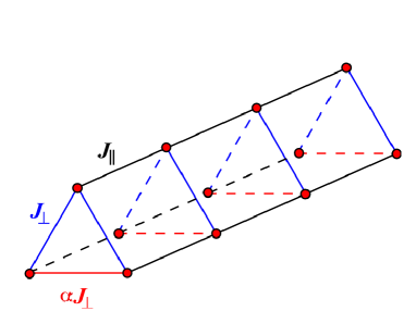
Figure 1: (color online) The three different parameters defining the coupling of the three-leg spin tube.

The point $\alpha=0$ corresponds to the unfrustrated open ladder while $\alpha=1$ is also special because of its translation symmetry in the transverse direction.

II.2 The classical case

We start by determining the classical configurations of spins which minimize the energy of each triangle by replacing the spin operators $\mathbf{S}_{a}$ with classical vectors $S\mathbf{n}_{a}$.

For $\alpha\geq 0.5$ the solutions that minimize the energy are of the kind of the coplanar solution of Figure 2 (b).

$$\mathbf{n}_{1}=\left(\begin{array}[]{c}\sin\theta\\ \rule[10.00002pt]{0.0pt}{5.0pt}0\\ \rule[10.00002pt]{0.0pt}{5.0pt}\cos\theta\\ \end{array}\right),\mathbf{n}_{2}=\left(\begin{array}[]{c}-\sin\theta\\ \rule[10.00002pt]{0.0pt}{5.0pt}0\\ \rule[10.00002pt]{0.0pt}{5.0pt}\cos\theta\\ \end{array}\right),\mathbf{n}_{3}=\left(\begin{array}[]{c}0\\ \rule[10.00002pt]{0.0pt}{5.0pt}0\\ \rule[10.00002pt]{0.0pt}{5.0pt}1\\ \end{array}\right),$$ (2)

with:

$$\cos\theta=-\frac{1}{2\alpha}.$$ (3)

In the extreme limit $\alpha\rightarrow\infty$, the two vectors $\mathbf{n}_{1}$ and $\mathbf{n}_{2}$ point in opposite direction and the third spin is essentially free. The system reduces then to the problem of one single chain. On the opposite, decreasing $\alpha$ one enters the regime $0\leq\alpha\leq 0.5$ in which the lowest energy state is an alternated collinear configuration of Figure 2(a). In this regime the physics becomes the one of an open unfrustrated ladder.

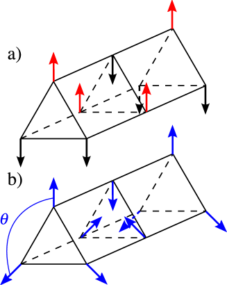
Figure 2: (color online) Top: The collinear configuration which minimizes the energy for $0\leq\alpha\leq 0.5$. Bottom: the coplanar configuration which minimizes the energy for $0.5\leq\alpha$.

Note that the collinear state and (2) are both continuously degenerate but have a different degree of degeneracy. For $0<\alpha\leq 0.5$, any alternated collinear configuration minimizes the energy. Thus, choosing a ground state is equivalent to picking up an oriented axis. For $0.5<\alpha$, all the classical ground states are given by a global rotation of the triad $(\mathbf{n}_{1},\mathbf{n}_{2},\mathbf{n}_{3})$. This, in turn, requires to choose an oriented axis and an angle.

II.3 Quantum spins : the decoupled limit

Introducing the triangle spin $\mathbf{J}=\mathbf{S}_{1}+\mathbf{S}_{2}+\mathbf{S}_{3}$ and the bond spin $\mathbf{S}_{12}=\mathbf{S}_{1}+\mathbf{S}_{2}$, the rung Hamiltonian reads:

$$\mathbf{S}_{i,3}\cdot\mathbf{S}_{i,1}+\mathbf{S}_{i,2}\cdot\mathbf{S}_{i,3}+\alpha\mathbf{S}_{i,1}\cdot\mathbf{S}_{i,2}$$

$$= \frac{J^{2}}{2}+(\alpha-1)\frac{{S_{12}}^{2}}{2}-(2\alpha+1)\frac{S(S+1)}{2}$$

$$= \frac{J(J+1)}{2}+(\alpha-1)\frac{S_{12}(S_{12}+1)}{2}-(2\alpha+1)\frac{S(S+1)}{2}$$

where we have replaced the spin operators by their eigenvalues. To determine the ground state, we need to label each state by their value of total spin $J$ and their intermediate spin $S_{12}$. For $\alpha=1$, the $S_{12}$ levels are degenerate and the ground state is obtained for the smallest value of $J$. Thus, the ground state is the singlet state $|0,S\rangle$ (if $J=0$, $S_{12}=S$ necessarily). When turning on the anisotropy, other levels will compete with this state. It is straightforward to show that the sequence of ground states $|J,S_{12}\rangle$ between $\alpha=1$ and $\alpha=0$ is:

$$|0,S\rangle\rightarrow|1,S+1\rangle\rightarrow...\rightarrow|S-1,2S-1\rangle\rightarrow|S,2S\rangle$$ (4)

The first level crossing happens for $\alpha=\frac{S}{1+S}$. The last level crossing occurs at $\alpha=0.5$. From this last result we can conclude that both, classically and quantum mechanically, the point $\alpha=0.5$ corresponds to the entrance into the unfrustrated open ladder regime given by $\alpha=0$. On the other side of the isotropic point, $\alpha\geq 1$, the sequence of ground state is given by:

$$|0,S\rangle\rightarrow|1,S-1\rangle\rightarrow...\rightarrow|S-1,1\rangle\rightarrow|S,0\rangle$$ (5)

The first crossing takes place at $\alpha=\frac{1+S}{S}$ and the last one occurs at $\alpha=1+S$. After this point, the triangle consists of two spins coupled into a singlet and an isolated spin. For instance, for $S=1$, there is a level crossing at $\alpha=0.5$ between the singlet state $|0,1\rangle$ and the triplet $|1,2\rangle$ and another one at $\alpha=2$ between the singlet and the triplet $|1,0\rangle$. On Figure 3, we plot the evolution of the main energy levels for $S=2$.

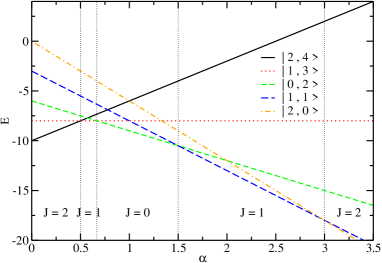
Figure 3: (color online) Spectrum of a single triangle for $S=2$ as a function of $\alpha$ as given by the two sequences (4) and (5). The higher energy levels are not represented.

Thus, in the strong rung coupling limit $J_{\parallel}=0$, there are $2S$ transition points in $0\leq\alpha\leq\infty$. If we now add a small longitudinal coupling $J_{\parallel}\ll J_{\perp}$, we can still expect that $2S+1$ different phases are present. However, we need to know how to effectively make the distinction between them. As we will see in the next chapter, this can be achieved with a non local string order parameter. The nature of the phases corresponding to $J=0$ and $J\neq 0$ are clearly different. In the former case, the tube just consists of a trivial superposition of singlets. We will refer to this phase as the singlet phase. In the latter, the properties of the tube are more similar to those of a single chain with $S=J$ spins, and we will refer to them as Haldane-like phases.

III Integer $S$ case and hidden symmetry

III.1 Hidden symmetry and string order parameters

In order to characterize the different phases suggested by the strong coupling analysis, we would like to find a suitable order parameter enabling us to describe the phase transitions. Usually, different phases are characterized by (local) order parameters, which detect spontaneous symmetry breakings. However, in some cases this standard approach does not work. This includes, in particular, the Haldane phase of $S=1$ chain: it has no local order parameter but still is a distinct phase separated from a trivial phase by a quantum phase transition. In order to characterize the Haldane phase, the non-local “string order parameters” Nijs , one of which is

$$\lim_{|k-i|\rightarrow\infty}\left\langle S^{z}_{i}\exp\left(i\pi\sum_{l=i}^{k-1}S_{l}^{z}\right)S^{z}_{k}\right\rangle,$$ (6)

is useful. It has been confirmed that it is non-vanishing within the Haldane phase but is zero in a trivial phase (for example the large anisotropy phase of Ref. Tasaki, ).

The problem with the non-local order parameter such as Eq. (6), in general, is that it is not quite clear if there is necessarily a phase transition between two states, when a non-local order parameter vanishes in one state but is non-zero in the other. Kennedy and Tasaki Kenn/Tasaki clarified the meaning of the string order parameter (6), as an order parameter measuring a spontaneous breaking of hidden discrete symmetry. Namely, there exists a non-local unitary transformation which transforms the Hamiltonian $\cal H$ to a Hamiltonian $\tilde{\cal H}$ with short-range interaction and with a discrete $\mathbb{Z}_{2}\times\mathbb{Z}_{2}$ symmetry. The $\mathbb{Z}_{2}\times\mathbb{Z}_{2}$ symmetry is hidden in a non-local way in the original Hamiltonian $\cal H$.

The string order parameter (6) is transformed by the same non-local unitary transformation to the standard ferromagnetic order parameter. Thus, non-vanishing string order parameter (6) implies a spontaneous breaking of the hidden $\mathbb{Z}_{2}\times\mathbb{Z}_{2}$ symmetry. The spontaneous symmetry breaking clearly distinguishes the phases. In this sense, the string order parameter indeed qualifies as an order parameter, despite its nonlocality.

The hidden $\mathbb{Z}_{2}\times\mathbb{Z}_{2}$ symmetry breaking also implies 4-fold groundstate degeneracy. This appears contradictory to the uniqueness of the groundstate in the Haldane phase. However, the non-local unitary transformation only works for the open boundary condition. Thus the hidden $\mathbb{Z}_{2}\times\mathbb{Z}_{2}$ symmetry breaking implies 4-fold groundstate degeneracy of the original Hamiltonian $\cal H$ only in the open boundary condition. This degeneracy actually corresponds to the existence of the edge states with spin $S_{b}=1/2$ at both ends.

The appearance of the edge states can be understood AKLT ; Kennedy ; Nijs ; Tasaki ; Kenn/Tasaki in the Valence Bond Solid (VBS) picture where each spin $1$ is seen as a triplet of spins $1/2$. Spin $1$ at each site is first decomposed into two spin $1/2$’s. Each constituent spin $1/2$ is then coupled to a spin $1/2$ in the neighboring site to form a singlet. This would give a simple dimerized state of a spin $1/2$ chain. However, projection to the triplet sector within each site gives a nontrival state for $S=1$ chain. If we consider this state on a finite chain with the open boundary condition, unpaired spin $1/2$ is left free at each end. Namely, spin $1/2$ degree of freedom appears at the ends. The above construction actually gives exact groundstates for a special, solvable Hamiltonian. For other models, the constructed state is of course not an exact groundstate. However, the appearance of the edge states is a common feature within the $S=1$ Haldane phase. As a consequence of the edge states, the groundstates of an open chain is asymptotically 4-fold degenerate. As mentioned above, this corresponds to the spontaneous breaking of the hidden $\mathbb{Z}_{2}\times\mathbb{Z}_{2}$ symmetry.

Thus, the hidden $\mathbb{Z}_{2}\times\mathbb{Z}_{2}$ symmetry breaking characterizes the $S=1$ Haldane phase, unifying the string order parameter and the edge states. However, it should be also noted that this picture is only valid in the presence of the global $\mathbb{Z}_{2}\times\mathbb{Z}_{2}$ symmetry. We will, in Sec. VIII, discuss from the perspective of recent, more general characterization of the Haldane phaseGuWen ; Pollmann09a .

Now let us move on to our problem of the spin tube with integer spin. Naturally, ladders/tubes are more complicated than the single chain, and various generalizations of the string order parameter have been proposed. However, as we have discussed for the single chain, generally there is no guarantee that a non-local “order parameter” really qualifies as an order parameter. Therefore, in this paper, we first generalize the hidden $\mathbb{Z}_{2}\times\mathbb{Z}_{2}$ symmetry to the tube. Then we identify the corresponding string order parameters, which detect spontaneous breaking of the hidden $\mathbb{Z}_{2}\times\mathbb{Z}_{2}$ symmetry.

Following Ref. Oshikawa, , the Kennedy-Tasaki transformation generalized to the tube can be written as:

$$V=\prod_{j<k}\exp\left(i\pi J^{z}_{j}J^{x}_{k}\right)$$ (7)

with $\mathbf{J}_{i}=\mathbf{S}_{i,1}+\mathbf{S}_{i,2}+\mathbf{S}_{i,3}$. We impose the open boundary condition on the tube (along the leg direction).

It is straightforward to show that the spin operators transform into:

$$VS^{x}_{i,a}V^{-1} =S^{x}_{i,a}\prod_{i<k}\exp\left(i\pi J^{x}_{k}\right)$$

$$VS^{y}_{i,a}V^{-1} =\prod_{k<i}\exp\left(i\pi J^{z}_{k}\right)S^{y}_{i,a}\prod_{i<k}\exp\left(i\pi J^{x}_{k}\right)$$

$$VS^{z}_{i,a}V^{-1} =\prod_{k<i}\exp\left(i\pi J^{z}_{k}\right)S^{z}_{i,a}$$

The natural generalization that comes to mind is to define the two string order parameters:

$$\langle\mathcal{O}^{x}\rangle =\lim_{|k-i|\rightarrow\infty}\left\langle J^{x}_{i}\exp\left(i\pi\sum_{l=i+1}^{k}J_{l}^{x}\right)J^{x}_{k}\right\rangle$$ (8)

$$\langle\mathcal{O}^{z}\rangle =\lim_{|k-i|\rightarrow\infty}\left\langle J^{z}_{i}\exp\left(i\pi\sum_{l=i}^{k-1}J_{l}^{z}\right)J^{z}_{k}\right\rangle$$ (9)

Applying the unitary transformation (7), they reduce to the local ferromagnetic order parameters:

$$\langle\tilde{\mathcal{O}}^{a}\rangle=\langle V\mathcal{O}^{a}V^{-1}\rangle=\lim_{|k-i|\rightarrow\infty}\langle J^{a}_{i}J^{a}_{k}\rangle,$$ (10)

for $a=x,z$. Now, let us consider the Hamiltonian. This transforms into:

$$\tilde{H} =\tilde{H}_{\parallel}+\tilde{H}_{\perp}$$ (11)

$$\tilde{H}_{\parallel} =J_{\parallel}\sum_{i}\left(\sum_{a=1,2,3}S^{x}_{i,a}S^{x}_{i+1,a}\right)\exp(i\pi J^{x}_{i})$$

$$+\left(\sum_{a=1,2,3}S^{z}_{i,a}S^{z}_{i+1,a}\right)\exp(i\pi J^{z}_{i+1})$$

$$+\left(\sum_{a=1,2,3}S^{y}_{i,a}S^{y}_{i+1,a}\right)\exp(i\pi(J^{x}_{i}+J^{z}_{i+1}))$$

$$\tilde{H}_{\perp} =J_{\perp}\left(\mathbf{S}_{i,1}\cdot\mathbf{S}_{i,3}+\mathbf{S}_{i,2}\cdot\mathbf{S}_{i,3}+\alpha\mathbf{S}_{i,1}\cdot\mathbf{S}_{i,2}\right)$$

Note that the rung part is invariant under the non-local transformation. The new Hamiltonian still consists of local interactions but the global continuous $SU(2)$ symmetry of the original Hamiltonian has been hidden and only a discrete $\mathbb{Z}_{2}\times\mathbb{Z}_{2}$ symmetry remains explicit: it is now only invariant under the rotation of all spins around the $x$ and $z$ axis by an angle of $\pi$.

We suggest that this “hidden” (non-local) symmetry and its associate string order parameters delineate the phases of the system. In the strong coupling limit ($J_{\parallel}\ll J_{\perp}$), the phase diagram of the spin tube consists of $2S+1$ phases, labelled by the spin index $J$, analogous to the Haldane state for a spin-$J$ chain. It has been demonstrated by one of us Oshikawa that not all Heisenberg spin chains, but only the ones with $J$ odd, do break the hidden $\mathbb{Z}_{2}\times\mathbb{Z}_{2}$ symmetry and possess a non zero string order parameter. Thus, as the anisotropy parameter $\alpha$ is varied in the spin tube (with $J_{\perp}\gg J_{\parallel}$), we will encounter a succession of phases with the string-order parameters (8)-(9) alternatively vanishing and non vanishing.

It is also interesting to consider a disorder parameter which detects unbroken hidden $\mathbb{Z}_{2}\times\mathbb{Z}_{2}$ symmetry, given as

$$\langle\mathcal{O}_{D}\rangle\equiv\lim_{|i-j|\rightarrow\infty}\left\langle\exp{\left(i\pi\sum_{l=i}^{j-1}J^{z}_{l}\right)}\right\rangle.$$ (12)

In fact, this was introduced in Ref. RiseFall, as a “parity correlation function” and shown to vanish in the Haldane phase but non-vanishing in a trivial phase. Here we discuss Eq. (12) from a different viewpoint from that in Ref. RiseFall, .

The non-local transformation (7) maps the non-local disorder parameter Eq. (12) to itself:

$$\langle V\mathcal{O}_{D}V^{-1}\rangle =\lim_{|i-j|\rightarrow\infty}\left\langle\exp{\left(i\pi\sum_{l=i}^{j-1}e^{i\pi\sum_{k<l}J^{z}_{k}}\tilde{J}^{z}_{l}\right)}\right\rangle$$

$$=\lim_{|i-j|\rightarrow\infty}\left\langle\exp{\left(i\pi\sum_{l=i}^{j-1}J^{z}_{l}\right)}\right\rangle,$$ (13)

where we used the fact that $\exp{(\pm i\pi J^{z})}=\exp{(i\pi J^{z})}$ because $J^{z}$ only takes integer values.

This correlation function can be interpreted as follows. The global $\pi$-rotation of spins (in the transformed basis) about $z$ axis is a generator of the $\mathbb{Z}_{2}\times\mathbb{Z}_{2}$ symmetry. Let us consider a localized operation, namely $\pi$-rotation about $z$ axis only on the spins in the finite section between $i$ and $j$. This “localized symmetry generator” is no longer a symmetry generator of the system. We apply this operation to the groundstate, and the overlap with the groundstate is measured. The limit $|i-j|\rightarrow\infty$ is taken afterwards. If the $\mathbb{Z}_{2}\times\mathbb{Z}_{2}$ symmetry is spontaneously broken, the application of the “localized symmetry generator” flips the order parameter in the finite section. Thus the overlap with the groundstate asymptotically vanishes in the limit $|i-j|\rightarrow\infty$. Therefore, the disorder parameter (12) vanishes if the hidden $\mathbb{Z}_{2}\times\mathbb{Z}_{2}$ symmetry is spontaneously broken. This is quite analogous to the well-known disorder parameter in the quantum transverse Ising chain. Kogut On the other hand, it does not vanish generically in a trivial phase where the hidden $\mathbb{Z}_{2}\times\mathbb{Z}_{2}$ symmetry is unbroken.

The discussion here implies that Eq. (12) acts as a disorder parameter for the hidden $\mathbb{Z}_{2}\times\mathbb{Z}_{2}$ symmetry, when the hidden $\mathbb{Z}_{2}\times\mathbb{Z}_{2}$ symmetry is well-defined. It would be the case even if the inversion (parity) symmetry is explicitly broken in the Hamiltonian, when the original argument in Ref. RiseFall, does not apply. (Although here we discussed the case of the tube, the same argument about the disorder operator applies to integer spin chains.)

III.2 Edge states

Possible quantum phases of the spin tube may be characterized by the hidden $\mathbb{Z}_{2}\times\mathbb{Z}_{2}$ symmetry breaking (or non-breaking). As in the case of single chain, spontaneous breaking of the hidden $\mathbb{Z}_{2}\times\mathbb{Z}_{2}$ symmetry implies 4-fold degeneracy of the groundstates, but only in the open boundary conditions. This implies the existence of the edge state (with half-integer spin, if the edge spin quantum number is well-defined.)

It also implies that, we can investigate whether the hidden $\mathbb{Z}_{2}\times\mathbb{Z}_{2}$ symmetry is spontaneously broken or not, by analyzing the existence of the edge states. If there are no edge states, the hidden $\mathbb{Z}_{2}\times\mathbb{Z}_{2}$ symmetry cannot be spontaneously broken. Existence of the edge state would suggest spontaneous breaking of the hidden $\mathbb{Z}_{2}\times\mathbb{Z}_{2}$ symmetry. However, it should be noted that the edge states could appear by a different mechanism unrelated to the hidden $\mathbb{Z}_{2}\times\mathbb{Z}_{2}$ symmetry.

The existence of the edge states can be analyzed easily in the strong-coupling limit ($J_{\parallel}\ll J_{\perp}$). In the strong coupling limit, we can project to the groundstates of each rung, which changes according to the sequence (4), as the tube anisotropy parameter $\alpha$ is varied.

Let us first discuss the $S=1$ tube. In the isotropic regime ($J_{\parallel}\ll J_{\perp}$ and $\alpha\sim 1$), each triangle tends to form singlets, and we thus expect a unique ground-state (with no boundary degeneracy) corresponding to the phase with unbroken $\mathbb{Z}_{2}\times\mathbb{Z}_{2}$. As this phase has no spin at the boundary, it will be referred as the $S_{b}=0$ phase. On the other hand, in the anisotropic, “unfrustrated” regime ($J_{\parallel}\ll J_{\perp}$ and $\alpha\lesssim 0.5$), the three spins of each triangle couple to form a $J=1$ spin object. The resulting physics is essentially that of the spin-1 chain and we expect a ground-state degeneracy due to the boundary spins. In the language of the transformed Hamiltonian this corresponds to the broken $\mathbb{Z}_{2}\times\mathbb{Z}_{2}$ phase with $\langle\mathcal{O}^{\alpha}\rangle\neq 0$. We will call this phase the $S_{b}=1/2$ phase in relation with the spin $1/2$ edge state of a spin-$1$ chain.

We can also discuss the edge states in the weak coupling limit ($J_{\parallel}\gg J_{\perp}$) with an heuristic argument. Taken separately, each chain of the tube is gapped, thus we can assume that a weak interchain coupling will not change qualitatively the physics in the bulk. On the contrary, solitary edge excitations of each of the three chains are expected to be very sensitive to any perturbation. As soon as a coupling $J_{\perp}$ is introduced, they will be bounded, leaving a unique spin-$1/2$ degree of freedom at each edge. This again corresponds to the $S_{b}=1/2$ phase, suggesting broken $\mathbb{Z}_{2}\times\mathbb{Z}_{2}$. This picture is valid for basically any non-zero value of $\alpha$. The only special point is $\alpha=1$ where the translation symmetry in the transverse direction leads to a bigger ${1\over 2}+{1\over 2}$ degeneracy space as it happens with three spin-$1/2$ with identical AF couplings.

III.3 Hidden $\mathbb{Z}_{2}\times\mathbb{Z}_{2}$ symmetry breaking in the weak coupling limit

The edge state analysis implies that the hidden $\mathbb{Z}_{2}\times\mathbb{Z}_{2}$ symmetry is spontaneously broken in the $S=1$ tube, in the weak coupling limit $J_{\perp}\ll J_{\parallel}$ for any value of $\alpha$.

However, there is a subtle issue in the weak coupling limit. It can be shown that the string order parameters (8) and (9) exactly vanish at the decoupling point $J_{\perp}=0$. At this point, the groundstate is given by a simple product of the groundstates of each chain. The string order parameter (8) can be decomposed as

$$\langle\mathcal{O}^{z}\rangle =\lim_{|k-i|\rightarrow\infty}\left\langle S^{z}_{i,1}\exp{\left(i\pi\sum_{l=i}^{k-1}S_{l,1}^{z}\right)}S^{z}_{k,1}\right\rangle_{1}\times$$

$$\left\langle\exp{\left(i\pi\sum_{l=i}^{k-1}S_{l,2}^{z}\right)}\right\rangle_{2}\times\left\langle\exp{\left(i\pi\sum_{l=i}^{k-1}S_{l,3}^{z}\right)}\right\rangle_{3}+\ldots,$$ (14)

where $\langle\rangle_{a}$ is the expectation value with respect to the groundstate of chain $a$. While there are $3\times 3=9$ terms, each one of them contains at least one factor of

$$\left\langle\exp{\left(i\pi\sum_{l=i}^{k-1}S_{l,a}^{z}\right)}\right\rangle_{a}.$$ (15)

This is nothing but the disorder operator for the single chain, introduced in Ref. RiseFall, and discussed in Sec. III.1. It vanishes because the ground state of each chain in the Haldane phase. As a consequence, the string order parameter (8) for the tube also vanishes, apparently implying that the hidden $\mathbb{Z}_{2}\times\mathbb{Z}_{2}$ symmetry is unbroken.

On the other hand, the disorder operator (12) also vanishes because it is simply a product of the disorder operators for the three chains. This rather suggests that the hidden $\mathbb{Z}_{2}\times\mathbb{Z}_{2}$ symmetry is spontaneously broken, in agreement with the edge state analysis.

The resolution of this apparent contradiction is as follows. The hidden $\mathbb{Z}_{2}\times\mathbb{Z}_{2}$ symmetry is indeed broken spontaneously even at the decoupling point $J_{\perp}=0$. However, the string order parameters (8) and (9), which are transformed to the ferromagnetic order in $J^{z,x}$ by the non-local unitary transformation (7), are not “good” order parameters to detect the symmetry breaking near the decoupling point.

In order to detect the hidden $\mathbb{Z}_{2}\times\mathbb{Z}_{2}$ symmery breaking around the decoupling point, we introduce the following variation of the string order parameter:

$$\langle\mathcal{O}^{zzz}\rangle=\lim_{|k-i|\rightarrow\infty}\left\langle S^{z}_{i,1}S^{z}_{i,2}S^{z}_{i,3}e^{i\pi\sum_{l=i}^{k-1}J_{l}^{z}}S^{z}_{k,1}S^{z}_{k,2}S^{z}_{k,3}\right\rangle.$$ (16)

The nonlocal transformation (7) maps this order parameter to a local order parameter

$$\langle V\mathcal{O}^{zzz}V^{-1}\rangle=\lim_{|k-i|\rightarrow\infty}\left\langle S^{z}_{i,1}S^{z}_{i,2}S^{z}_{i,3}S^{z}_{k,1}S^{z}_{k,2}S^{z}_{k,3}\right\rangle.$$ (17)

This does measure spontaneous breaking of the $\mathbb{Z}_{2}\times\mathbb{Z}_{2}$ symmetry because $S^{z}_{i,1}S^{z}_{i,2}S^{z}_{i,3}$ is odd under the global $\pi$-rotation about $x$ axis.

At the decoupled point $J_{\perp}=0$, Eq. (16) reduces to the product of the standard string order parameter (6) for the independent chains. Since Eq. (6) is non-vanishing in the groundstate of each chain, the “product” string order parameter (16) is also non-vanishing in the tube at the decoupling point. Therefore, the hidden $\mathbb{Z}_{2}\times\mathbb{Z}_{2}$ symmetry is indeed spontaneously broken even at the decoupled point $J_{\perp}=0$, although the string order parameters (8) and (9) cannot detect the symmetry breaking. The edge spin $S_{b}=1/2$ in the weak coupling limit, as well as in the strong coupling limit with anisotropy $\alpha\lesssim 0.5$, can be understood as a consequence of the hidden $\mathbb{Z}_{2}\times\mathbb{Z}_{2}$ symmetry breaking. Thus no phase transition is expected between these two regions, as both of them would belong to the hidden $\mathbb{Z}_{2}\times\mathbb{Z}_{2}$ symmetry broken phase.

We note that the “product” string order parameter (16) is very similar to the $\mathcal{O}_{4}$ defined in Eq. (19) of Ref. Todo, . However, there is a crucial difference between the two-leg $S=1$ ladder case studied in Ref. Todo, and the three-leg ladder/tube case discussed in this paper. In the present case, the “product” string order parameter detects spontaneous breaking of the hidden $\mathbb{Z}_{2}\times\mathbb{Z}_{2}$ symmetry, thanks to the relation eq. (17). However, in the two-leg ladder case, we find:

$$V\mathcal{O}_{4}V^{-1}=\mathcal{O}_{4}.$$ (18)

Thus $\mathcal{O}_{4}$ introduced in Ref. Todo, does not detect hidden $\mathbb{Z}_{2}\times\mathbb{Z}_{2}$ symmetry breaking.

In general, the product of string order parameters of each chain is an order parameter for the hidden $\mathbb{Z}_{2}\times\mathbb{Z}_{2}$ symmetry breaking in integer-spin ladder/tube with an odd number of legs, but not with an even number of legs. As a consequence, the hidden $\mathbb{Z}_{2}\times\mathbb{Z}_{2}$ symmetry (defined with respect to Eq. (7)) is broken in the weak rung coupling limit of the odd-leg ladder/tube with an odd integer spin, but remains unbroken in the same limit if either the spin or the number of legs is even.

III.4 Conjectured phase diagrams for $S=1$ and $S=2$

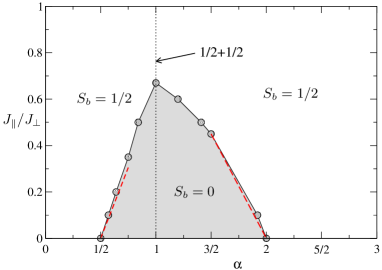
Figure 4: (color online) Numerical phase diagram for the spin $1$ tube obtained with DMRG (see part VI.2). Both phases can be distinguished according to the string order parameters $\mathcal{O}^{z}$ (see Eq.(9) or (16)) and part VI.2.1). The label $S_{b}$ for the different phases stands for the value of the spin of the boundary state for OBC. The transition between the $S_{b}=0$ and $S_{b}=1/2$ regime is analyzed in more detail in this paper and turns out to be first order. Phase boundaries obtained from an effective model (see part VI.1) are also shown with dashed red lines and agree quite well with numerical results.

Let us now discuss the phase diagram. Here we propose the simplest phase diagram consistent with our analyses in the previous subsections. In Figure 4, we show the conjectured/numerical phase diagram for a $S=1$ spin tube as a function of $J_{\parallel}$ and $\alpha$. In one of the two phases, the hidden $\mathbb{Z}_{2}\times\mathbb{Z}_{2}$ symmetry is spontaneously broken and the edge state with $S_{b}=1/2$ appears. Although there are more edge state degeneracy on the special lines $\alpha=1$ and $J_{\perp}=0$, these lines are also a part of the broken hidden $\mathbb{Z}_{2}\times\mathbb{Z}_{2}$ symmetry phase.

This phase diagram is also confirmed by numerical simulations; the details will be given in Sec. VI.2.

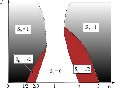
Figure 5: (color online) Sketch of the phase diagram for the $S=2$ spin tube. Again, the label $S_{b}$ for the different phases stands for the value of the spin of the boundary state. The $S_{b}=1/2$ phases (light red) must be separated from the others with real phase transitions (full lines). On the other hand, there is no reason to expect a real phase transition between the regions $S_{b}=0$ and $S_{b}=2$ so we have plotted these boundaries with dash-dotted lines.

We can also conjecture the phase diagram for the $S=2$ spin tube, as in figure 5. Based on the strong coupling analysis, we in principle expect three different phases: a singlet phase with no edge states, centered around $\alpha=1$, one phase with $1/2$ boundary states, and two phases with $S_{b}=1$ boundary spins. We can also discuss the weak rung coupling limit $J_{\perp}\rightarrow 0$ in terms of edge states, by repeating the calculation of the decoupled triangle of the preceding section but by this time reasoning on the edge $S=1$ spins of the three $S=2$ chains. We conclude, at the decoupling point $J_{\perp}=0$, that there are no edge states for $0.5<\alpha<2$ and that there should be a single spin $S_{b}=1$ at the boundaries for any other value of the anisotropy parameter.

The edge state with $S_{b}=1/2$ would correspond to a spontaneous symmetry breaking of the hidden $\mathbb{Z}_{2}\times\mathbb{Z}_{2}$ symmetry, which clearly characterizes a distinct phase from those with $S_{b}=0,1$. The phase with $S_{b}=1$ also appears to be different from the $S_{b}=0$, concerning the edge state. However, there is in principle no way to distinguish the phases with $S_{b}=0$ and $S_{b}=1$. This is suggested by the fact that hidden $\mathbb{Z}_{2}\times\mathbb{Z}_{2}$ symmetry is unbroken in the $S=2$ Haldane “phase”.Oshikawa In fact, it was pointed out recently in Ref. Pollmann09a, that the $S=2$ Haldane “phase” with $S_{b}=1$ is adiabatically connected to a trivial phase with $S_{b}=0$.

In our problem, the $S_{b}=0$ and $S_{b}=1$ “phases” are certainly adiabatically connected at the decoupled point $J_{\perp}=0$, where the system is just a collection of three $S=2$ chains with the Haldane gap. With an infinitesimal coupling $J_{\perp}$, the gap should not close for any value of $\alpha$. Therefore we expect that $S_{b}=0$ and $S_{b}=1$ “phases” actually belong to a single phase in which the hidden $\mathbb{Z}_{2}\times\mathbb{Z}_{2}$ symmetry is unbroken.

IV The large $S$ limit: non Linear $\sigma$ model

IV.1 Long wavelength description of the spin tube

Having first examined the system from the strong coupling perspective, we now shift to the examination of the large-$S$ approaches whose greatest achievements culminate with the non linear sigma model. The latter has shown to be particularly important in order to distinguish the nature of the ground state, the low energy excitations and the possible critical points of an antiferromagnet Manousakis ; CHN ; Johannesson . It thus proves valuable to conduct such a study here to complete our previous analysis. The NL$\sigma$M can be derived from the Heisenberg model when the spin $S$ is large. In principle, it does not make any distinction between integer and half-integer spins, as $S$ is just one between multiple parameters allowed to flow continuously to their renormalized values at long wavelength. However, the parity of the spin profoundly influences the value of the Berry phase, a purely quantum quantity originating from non zero overlaps between coherent states and entering the NL$\sigma$M action. As shown by Haldane Haldane1983 , the value of the Berry phase eventually governs the properties of the system in the infrared limit.

Although the spin-wave expansion cannot make good quantitative predictions on a magnetic model in one dimension, it is useful to carry this analysis in order to identify the low-energy, long-wavelength degrees of freedom in the spin tube. These degrees of freedom will help later on to construct a well-defined order parameter for the NL$\sigma$M. A standard spin wave analysis shows that there are three low energy modes depicted in Figure (6) and their canonical conjugate.

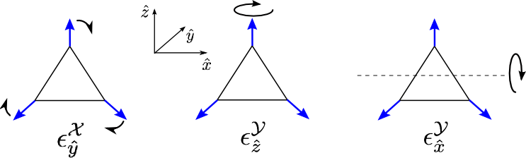
Figure 6: (color online) The low energy modes deduced from the linear spin wave theory are connected to the three rotations of the initial triad around the axis $\hat{x},\hat{y},\hat{z}$. When propagating to the tube, they underpin slow twists of the original structure which asymptotically cost no energy at long wavelengths.

With the expression of the low-energy modes $\epsilon^{\mathcal{X}}_{\hat{y}}$, $\epsilon^{\mathcal{Y}}_{\hat{z}}$ and $\epsilon^{\mathcal{Y}}_{\hat{x}}$, and their respective conjugate modes $\epsilon^{\mathcal{Y}}_{\hat{y}}$, $\epsilon^{\mathcal{X}}_{\hat{z}}$ and $\epsilon^{\mathcal{X}}_{\hat{x}}$, we can reexpress the slowly varying spin degrees of freedom. The spin operators can be rewritten in a compact form by introducing an infinitesimal $SO(3)$ rotation matrix $\mathcal{R}_{i}=\exp\left(i\mathbf{m}_{i}\hat{\mathbf{J}}\right)$ with $\hat{\mathbf{J}}$ standing for the generator of $SO(3)$, and a vector $\mathbf{L}_{i}$ if we identify:

$$\mathbf{L}=\left(\begin{array}[]{c}\frac{-2\alpha}{\sqrt{4\alpha^{2}+2}}\epsilon^{\mathcal{X}}_{\hat{x}}\\ \rule[10.00002pt]{0.0pt}{5.0pt}\frac{\epsilon^{\mathcal{Y}}_{\hat{y}}}{3}\\ \rule[10.00002pt]{0.0pt}{5.0pt}-\frac{\epsilon^{\mathcal{X}}_{\hat{z}}}{\sqrt{2-\frac{1}{2\alpha^{2}}}}\\ \end{array}\right)\;\;\;\mathbf{m}=i\left(\begin{array}[]{c}\frac{2\alpha}{\sqrt{4\alpha^{2}+2}}\epsilon^{\mathcal{Y}}_{\hat{x}}\\ \rule[10.00002pt]{0.0pt}{5.0pt}\frac{\epsilon^{\mathcal{X}}_{\hat{y}}}{3}\\ \rule[10.00002pt]{0.0pt}{5.0pt}\frac{\epsilon^{\mathcal{Y}}_{\hat{z}}}{\sqrt{2-\frac{1}{2\alpha^{2}}}}\\ \end{array}\right).$$

The original spin operators read very simply:

$$\mathbf{S}_{i,a}=(-1)^{i}\mathcal{R}_{i}\mathbf{n}_{a}+(\mathbf{L}_{i}-(\mathbf{L}_{i}\cdot\mathbf{n}_{a})\mathbf{n}_{a}).$$ (19)

where the vectors $\mathbf{n}_{a}$ are given in (2). The number of degrees of freedom on the left and on the right hand side of this equation is the same. Thus, this operation can be regarded as a simple change of variables, but if one is interested in a long wavelength limit, the new variables $\mathcal{R}_{i}$ and $\mathbf{L}_{i}$ are the most adapted to describe the physics of the anisotropic spin tube.

IV.2 Derivation of the NL$\sigma$M

After having derived the low energy modes of the theory, we can now focus on the construction of the NLsM. The first point is to define a suitable local order parameter. In the case of a coplanar configuration, the role of the order parameter will be played by the $SO(3)$ rotation matrix. The underlying idea behind the construction of the NLsM is then to consider the system in its symmetry-broken phase and to take into account quantum fluctuations around the direction of the order parameter. It is actually not necessary that the system admits a broken-symmetry phase (it has none in $1d$), it just needs to be at least ordered locally, which is the case in the weak rung coupling limit $J_{\parallel}\gg J_{\perp}$. The continuum limit is then reached within a Hamiltonian formalism or a path integral (lagrangian) approach Fradkin . One of the greatest possibilities given by the NLsM is that it can be investigated with renormalization group techniques for which one can determine the nature of the possible fixed points governing the physics at long wavelengths. The quantum NLsM for triangular geometries and its RG analysis have already been extensively studied by Azaria et al. Azaria ; Mouhanna . We shall refer later to their work for the characterization of the spectrum. For now, our starting point will be different. We will build the NLsM in the lagrangian formalism, following the construction of Dombre and Read Dombre . This path integral approach is particularly illustrative regarding the construction of the Berry phases. These complex terms will play a major role in our analysis of the quantum spin tube.

In the long wavelength limit, the fine scale of the lattice becomes irrelevant and the lattice spacing $\lambda$ can be taken to zero. To obtain a well-defined continuum limit, we need to choose a local order-parameter field which has a smooth spatial variation on the scale of $\lambda$. To do so, we make use of the following ansatz Dombre :

$$\mathbf{S}_{i,a}(t)=S\frac{\mathcal{R}_{i}(t)\left((-1)^{i}\mathbf{n}_{a}+\lambda\mathbf{L}_{i}(t)\right)}{|\mathcal{R}_{i}(t)\left((-1)^{i}\mathbf{n}_{a}+\lambda\mathbf{L}_{i}(t)\right)|},$$ (20)

where the fields $\mathcal{R}$ and $\mathbf{L}$ depend on the time $t$ and the lattice coordinate $i$. This is identical to (19) at first order in $\lambda$. Here however, to make a coherent calculation, we will need to keep the development up to second order in $\lambda$:

$$\mathbf{S}_{i,a} \approx S\mathcal{R}_{i}\left((-1)^{i}\mathbf{n}_{a}+\lambda(\mathbf{L}_{i}-(\mathbf{n}_{a}.\mathbf{L}_{i})\mathbf{n}_{a})\right.$$

$$+ \left.(-1)^{i}\lambda^{2}\left(\left(-\frac{\mathbf{L}_{i}^{2}}{2}+\frac{3}{2}(\mathbf{n}_{a}.\mathbf{L}_{i})^{2}\right)\mathbf{n}_{a}-(\mathbf{n}_{a}.\mathbf{L}_{i})\mathbf{L}_{i}\right)\right).$$

In particular, the square of the magnetization of the whole triad is given by:

$$\left(\sum_{a}\mathbf{S}_{i,a}\right)^{2}\approx S^{2}\left(\frac{\alpha-1}{\alpha}\right)^{2}+9\lambda^{2}S^{2}(T\mathbf{L}_{i})^{2}+$$

$$\lambda^{2}S^{2}\left(\frac{\alpha-1}{\alpha}\right)^{2}\left(-\mathbf{L}_{i}^{2}-2{L_{i}^{z}}^{2}+3\frac{\alpha}{1-\alpha}\sum_{a}(\mathbf{n}_{a}.\mathbf{L}_{i})^{2}(\mathbf{n}_{a}.\hat{z})\right),$$

where $T_{\alpha\beta}=\delta_{\alpha\beta}-\frac{1}{3}\sum_{a}n_{a\alpha}n_{a\beta}$, and $(T\mathbf{L})_{\alpha}=\sum_{\beta}T_{\alpha\beta}L_{\beta}$. We set again $J_{\parallel}=J_{\perp}=1$ for simplicity and concentrate on the effects of the anisotropy parameter $\alpha$. The action we wish to estimate is Fradkin :

$$S_{{\rm NL}\sigma{\rm M}} =S_{BP}+S_{H}$$

$$=i\sum_{i,a}\omega[\mathbf{S}_{i,a}]-\int\textrm{d}\tau H[\mathbf{S}_{i,a}],$$ (22)

$\tau$ denoting imaginary time. The first part of the action is the Berry phase term. It measures the total area covered by each of the spins $\mathbf{S}_{i,a}$ on the sphere of radius $S$. Up to second order, the Berry phase term reads:

$$S_{BP}=iS\sum_{i,a}(-1)^{i}\omega[\mathcal{R}_{i}\mathbf{n}_{a}]+i3S\int\textrm{d}\tau\textrm{d}x\;\left(T\mathbf{L}_{i}\right)\cdot\mathbf{V},$$ (23)

where $V_{\alpha}=-\frac{1}{2}\epsilon^{\alpha\beta\gamma}(\mathcal{R}^{-1}\partial_{\tau}\mathcal{R})_{\beta\gamma}$ and $\epsilon^{\alpha\beta\gamma}$ is the totally antisymmetric tensor. The first member of the right-hand side,

$$S^{\prime}_{BP}=iS\sum_{i,a}(-1)^{i}\omega[\mathcal{R}_{i}\mathbf{n}_{a}]$$ (24)

takes a particular significance when one allows for the possibility of singularities in the action. These singularities are naturally present in the system because we start from a lattice description with discrete variables and not fields. However, we wish not to take them into account now and we will let apart this term for the moment. We will reconsider it when evaluating the role of the topological defects in the theory.

The second member of Eq. ((22)) is nothing but the Hamiltonian (1) where the quantum spin operators have been replaced by the ansatz (IV.2). The Hamiltonian part, at second order in $\lambda$, reads:

$$S_{H} =\int\textrm{d}x\textrm{d}\tau\left(-\frac{1}{\lambda}S_{\rm triad}-6\lambda S^{2}T\mathbf{L}(x,\tau)\cdot\mathbf{L}(x,\tau)\right.$$

$$+S\left.\textrm{Tr}[P(\mathcal{R}(x,\tau)^{-1}\partial_{x}\mathcal{R}(x,\tau))^{2}]\right).$$

with:

$$S_{\rm triad}=\frac{1}{2}\left(\sum_{a}\mathbf{S}_{i,a}\right)^{2}-\frac{1-\alpha}{2}\left(\mathbf{S}_{i,1}+\mathbf{S}_{i,2}\right)^{2}.\\$$

Since the action is quadratic in the field $\mathbf{L}(x,\tau)$, we can integrate the field out and finally express the action solely in terms of the $SO(3)$ matrix field $\mathcal{R}(x,t)$:

$$S_{\rm NL\sigma M} = S\int\textrm{d}x\textrm{d}\tau\,\left(\textrm{Tr}[P(\mathcal{R}(x,\tau)^{-1}\partial_{x}\mathcal{R}(x,\tau))^{2}]\right.$$ (25)

$$+ \left.\textrm{Tr}[Q(\mathcal{R}(x,\tau)^{-1}\partial_{\tau}\mathcal{R}(x,\tau))^{2}]\right)+iS^{\prime}_{BP}.$$

Here $P$ and $Q$ are diagonal matrices whose expression is better given by the spin-stiffness and susceptibility tensors Azaria :

$$\chi_{\alpha\beta}=-\textrm{Tr}(Qt_{\alpha}t_{\beta}),\hskip 14.22636pt\rho_{\alpha\beta}=-\textrm{Tr}(Pt_{\alpha}t_{\beta}),$$ (26)

with $\chi_{\alpha\beta}=\chi_{\alpha}\delta_{\alpha\beta}$, $\rho_{\alpha\beta}=\rho_{\alpha}\delta_{\alpha\beta}$ and:

$$\chi_{1} = \frac{S(1+2\alpha^{2})^{2}}{\lambda\alpha(1+4\alpha(3+\alpha+4\alpha^{2}))},\;\chi_{2}=\frac{9S\alpha}{\lambda(2+8\alpha(4+\alpha))},$$

$$\chi_{3} = \frac{S}{\lambda}\left(\frac{1}{\alpha}-\frac{8}{-1+4\alpha(2+\alpha)}\right),$$

$$\rho_{1} = \lambda S\left(1+\frac{1}{2\alpha^{2}}\right),\;\rho_{2}=3\lambda S,\;\rho_{3}=\lambda S\left(2-\frac{1}{2\alpha^{2}}\right).$$ (27)

Here $t_{\alpha}$ are the generators of the $SO(3)$ group. Finally, we introduce the fields $\mathcal{R}(x,\tau)^{-1}\partial_{\mu}\mathcal{R}(x,\tau)=\omega^{\alpha}_{\mu}t_{\alpha}$. The action reads note-velocity :

$$S_{\rm NL\sigma M}=\frac{S}{2}\int_{0}^{\infty}\textrm{d}\tau\textrm{d}x\left(\chi_{\alpha\beta}\omega_{0}^{\alpha}\omega_{0}^{\beta}+\rho_{\alpha\beta}\omega_{x}^{\alpha}\omega_{x}^{\beta}\right)+iS^{\prime}_{BP},$$ (28)

IV.3 Bare analysis of the NL$\sigma$M.

The two formulations of the action, eqs. (25) and (28), are valid for all $\alpha\geq 0.5$. In particular, we should be able to recover the isotropic limit $\alpha=1$, and the unfrustrated cases $\alpha=0.5$ and $\alpha\rightarrow\infty$. For $\alpha=1$, one notes that $\rho_{1}=\rho_{3}\neq\rho_{2}$ and $\chi_{1}=\chi_{3}\neq\chi_{2}$. In the language of the $SO(3)$ matrices, this translates into an additional $SO(2)$ global right symmetry of the action: $\mathcal{R}\rightarrow\mathcal{R}U_{R}$. This symmetry is reminiscent of the discrete $C_{3v}$ symmetry of the triangle for $\alpha=1$. Since the configurations of fields classically minimizing the action also possesses a $SO(2)$ symmetry, this model is referred to as the $SO(3)\times SO(2)/SO(2)$ NL$\sigma$M Delduc ; Azaria . When $\alpha=0.5$, one finds $\rho_{1}=\rho_{2}$, $\chi_{1}=\chi_{2}$ and $\chi_{3}=\rho_{3}=0$ and recovers the description of the collinear antiferromagnet in terms of a $O(3)/O(2)$ NL$\sigma$M.

There is another, third representation of the action (25)-(28) that nicely illustrates the effect of the anisotropy parameter $\alpha$. Remembering that a $SO(3)$ matrix is nothing more but a set of three orthonormal vectors: $(\mathbf{e}_{b})_{a}=\mathcal{R}_{ab}$, we can use the fact that $\mathbf{e}_{2}=\mathbf{e}_{3}\times\mathbf{e}_{1}$ to rewrite the bare action in terms of two orthonormal unit vectors:

$$S_{\rm NL\sigma M} = S_{1}+S_{3}+S_{\textrm{coupling}}+S^{\prime}_{BP},$$ (29)

$$S_{a} = \frac{1}{2\tilde{g}_{a}}\int\textrm{d}x\textrm{d}\tau\left(\tilde{c}_{a}(\partial_{\tau}\mathbf{e}_{a})^{2}+\frac{1}{\tilde{c}_{a}}(\partial_{x}\mathbf{e}_{a})^{2}\right),$$

$$S_{\textrm{coupling}} = -\frac{\kappa}{2}\int\textrm{d}x\textrm{d}\tau(\mathbf{e}_{3}\cdot\partial_{\tau}\mathbf{e}_{1})^{2},$$

where the new constants can be easily expressed as a function of the spin-stiffness and susceptibility tensors. The behavior of the different couplings as a function of $\alpha$ are easily obtained from the expression of the spin-stiffness and susceptibility tensors. An important point is that for $\alpha\to 0.5$, $g_{1}\to\infty$ and $\kappa\to 0$ i.e. when $\alpha=0.5$ the $\mathbf{e}_{1}$ field becomes a spurious degree of freedom with null stiffness! This is consistent with the collinear picture in the range $0\leq\alpha\leq 0.5$. Such a model is in fact well described by the fluctuations of a single unit vector $\mathbf{e}_{3}$.

IV.4 Renormalization group analysis of the NL$\sigma$M.

The above bare analysis of the NL$\sigma$M is insufficient to describe properly the behavior of the spin tube in the infrared limit. As it is well known from the study of the quantum spin chain, quantum fluctuations always renormalize the parameters entering a NL$\sigma$M action and eventually drive the system into a quantum disordered state in $1d$ Polyakov . Thus, in order to understand the properties of the system at long wavelength, one must perform a renormalization group analysis to determine how do the different coupling constants (27) renormalize. We are going to use the results for the one-loop RG equationsAzaria ; Mouhanna , starting with the set of bare couplings (27). To make the distinction between isotropic and anisotropic cases, we introduce the two anisotropy parameters $\alpha_{2}=1-\rho_{2}/\rho_{1}$ and $\alpha_{3}=1-\rho_{3}/\rho_{1}$ and the coupling $g=2/\rho_{1}$, the latter playing the role of an effective coupling constant. The set of couplings $\gamma=\{c_{1},c_{2},c_{3},\alpha_{2},\alpha_{3},g\}$ obeys the general RG equations:

$$\frac{\partial\gamma}{\partial l}=-\beta(\{\gamma\})$$ (30)

We have integrated numerically these equations for different values of $\alpha$ ranging from $\alpha=0.55$ to $\alpha=0.95$ (similar behaviors were also observed for values above $\alpha=1$). The numerical integration of the RG equations yields the unambiguous result that the symmetry is dynamically enlarged in the infrared limit, similarly to the higher dimensional cases. For any value of $\alpha>0.5$, the spin wave velocities renormalize to the same value $c_{1}^{\star}=c_{2}^{\star}=c_{3}^{\star}$ while the two anisotropy parameters $\alpha_{2}$ and $\alpha_{3}$ fall to zero. The symmetry of the model in the long-wavelength limit is therefore $SO(3)\times SO(3)/SO(3)\approx SO(4)/SO(3)$. The coupling $g$ diverges, as one could have expected in one dimension. Hence, there seems to be no qualitative differences between the cases $\alpha=1$ and $\alpha>0.5,\alpha\neq 1$ at the one loop level, suggesting that a deviation from the point $\alpha=1$ is an irrelevant perturbation. However, we have not taken into account so far the role of the Berry phase term, which as we are going to see plays an important role when $\alpha\neq 1$.

V Berry phases and Instantons

V.1 Instantons in SO(3) NL$\sigma$M

The continuous part of the sigma model does not make any distinction between the integer and the half-integer quantum spin tube. In fact, the preceding RG equations suggest that the model is gapped in both cases, and admits a unique ground state for any $\alpha$. Nonetheless, the DMRG data show unambiguously a dimerization of the ground state of the spin tube for $S=\frac{1}{2}$ at $\alpha=1$ Sakai ; Nishimoto . Analogously, the Majumdar-Gosh model, whose NL$\sigma$M also has the $SO(3)\times SO(2)/SO(2)$ symmetry, is dimerized Majumdar ; Rao . In a single spin chain, the difference between integer and half-integer spins can be explained in the NL$\sigma$M by the presence of a topological term in the action Haldane1983 . Here, such a term is absent because of the triviality of the second homotopy group of the $SO(3)$ manifold Dombre ; Mermin :

$$\pi_{2}(SO(3))=0$$

However, only continuous space-time configurations of the field $\mathcal{R}(x,\tau)$ have been considered up to now. In fact, there also exist configurations containing vortices with singular cores. These defects originate from the non trivial first homotopy group of $SO(3)$:

$$\pi_{1}(SO(3))=\mathbf{Z}_{2}.$$ (31)

For classical antiferromagnets on the triangular lattice, these vortices are argued to be the driving force of a phase transition Miyashita .

In quantum systems, topological defects radically affect the behavior of the disordered phases of the $O(3)/O(2)$ NL$\sigma$M in $2d$ Haldane1988 , leading the system to dimerization, and of the $SO(3)\times SO(2)/SO(2)$ NL$\sigma$M in $1d$ Rao . The specificity of our system is that the $SO(2)$ symmetry is, at least at the bare level, no longer present when $\alpha\neq 1$. Thus, we would like to investigate the conjugate action of the topological defects, also known as instantons Polyakov , and of the anisotropy in the spin tube. For integer $S$, we will see that the presence of the topological defects gives rise to the emergence of $2S$ peculiar values of $\alpha$, that we could associate with the critical points determined from the strong coupling approach.

We would like to review first the nature of the instantons in our system. Instantons are topological defects associated to the symmetry group of the order parameter. The $SO(3)$ group manifold is isomorphic to a ball of radius $\pi$ in three dimensions whose diametrically opposite points on the surface are identified. One can associate to a rotation around an axis $\mathbf{n}$ by an angle $\theta$, the vector $\theta\mathbf{n}$ with $\theta\in[-\pi,\pi]$. The redundancy between two opposite points on the surface of the sphere stems from the identification between a rotation about an axis $\mathbf{n}$ of angle $\pi$ and the rotation about the same axis of angle $-\pi$. It is then clear that the $SO(3)$ manifold is non simply connected, with the ensemble of closed path in $SO(3)$ dividing into two classes: one containing the loops shrinkable to a point, the other ones containing strings joining two opposite points of the ball. This is equivalent to say that the first homotopy group of the $SO(3)$ manifold is given by (31). Considering the evolution of a matrix $\mathcal{R}(x)$ through space, an element of the non trivial class is:

$$\mathcal{R}(t)=\left(\begin{array}[]{ccc}\cos\theta(x)&\sin\theta(x)&0\\ -\sin\theta(x)&\cos\theta(x)&0\\ 0&0&1\\ \end{array}\right),$$ (32)

with $\theta(x=0)=0$ and $\theta(x=L)=2\pi$, where $L$ is the size of the system. Conversely, the trivial class will consist of matrices which stay close to the identity matrix at all positions.

Turning back to our $1+1$ dimensional problem, suppose now we start from a configuration in the trivial sector with all $\mathbf{e}_{1}$ vectors pointing up and all $\mathbf{e}_{2}$ vectors pointing right, where again $\mathcal{R}_{\alpha\beta}=(\mathbf{e}_{\alpha})_{\beta}$ (see Fig 7). If nothing ”sudden” happens, i.e. if the time evolution process is sufficiently smooth, the chain should visit other configurations but stay in the trivial topological class. However, it is also possible that some non trivial configurations arise during time evolution that will connect the two classes of path. These are the instantons. A pair of instanton (going from the trivial to the non-trivial class) and anti-instanton (i.e the opposite) is represented on Fig. 7. In the continuum, an instanton will appear as a singularity. It is clear that such an event is unlikely to happen if the tube is ordered. However, since the model is disordered at long wavelengths, these events will eventually proliferate. Now, it may be that the proliferation of instantons is constrained by the Berry phase term. Here, we would like to calculate:

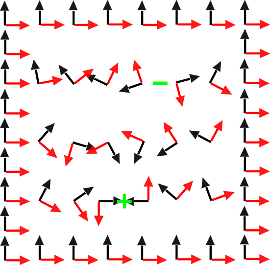
Figure 7: (color online) Evolution of the spin tube from the two different topological sectors of $SO(3)$. Each triad is represented by two orthonormal vectors $\mathbf{e}_{1}(x,t)$ and $\mathbf{e}_{2}(x,t)$ that one can connect with the classical configuration of spins on each triangle $(\mathbf{S}_{i,1},\mathbf{S}_{i,2},\mathbf{S}_{i,3})$ Delduc . In the continuum, $\mathbf{e}_{1}$ and $\mathbf{e}_{2}$ also stand for the first two vector columns of the rotation matrix $\mathcal{R}(x,t)$. Starting from a Néel configuration, the system tunnels to a non trivial configuration via an instanton event $(+)$. The system returns to the trivial configuration via an anti-instanton $(-)$.

$$S^{\prime}_{BP}=iS\sum_{i,a}\omega[\mathcal{R}_{i}\mathbf{n}_{a}](-1)^{i}.$$ (33)

which is the discrete part of the total Berry phase (23) that we let apart. For this purpose, we follow Dombre and Read again and consider a first time path $\mathcal{R}(\tau)$ satisfying the closed boundary conditions and a second one $\mathcal{R}^{\prime}(\tau)=\mathcal{R}(\tau)+\delta\mathcal{R}(\tau)$ infinitesimally close to $\mathcal{R}(\tau)$. The difference of Berry phases between the two paths can be easily evaluated to be:

$$\delta S^{\prime}_{BP} = iS\int\textrm{d}\tau\sum_{a}(\delta\mathcal{R}\mathbf{n}_{a})\cdot(\partial_{\tau}\mathcal{R}\mathbf{n}_{a}\times\mathcal{R}\mathbf{n}_{a})$$

$$= -iS\int\textrm{d}\tau V_{\beta}(\mathcal{R}^{-1}\delta\mathcal{R})_{\beta\beta^{\prime}}\left(\sum_{a}\mathbf{n}_{a\beta^{\prime}}\right).$$

V.2 Isotropic case, $\alpha=1$

In the isotropic case, we have the important result that:

$$\delta S^{\prime}_{BP}=0$$ (34)

and any smooth change in the history of $\mathcal{R}(\tau)$ will not change the value of the Berry phase of the triad. Thus, this quantity can be used to index the two classes of $\pi_{1}(SO(3))$, exactly like the hedgehog number classifies the configurations of the spins in two dimensions Haldane1983 ; Fradkin . Because the quantity is a topological invariant, we just need to calculate it for one path representing each class. For the trivial class, we can take the identity matrix so that $\sum_{a}\omega[\mathcal{R}(t)\mathbf{n}_{a}]=0\,[4\pi S]$. For the non-trivial class, we can consider the rotation of the triad around an arbitrary axis. In this case, the Berry phase of the triad will be $2\pi S\,[4\pi S]$. So, the alternating sum (33) reads:

$$S^{\prime}_{BP}=iS\sum_{i,a}2\pi q_{i}(-1)^{i},$$ (35)

where $q_{i}=0,1$ depending on which class the matrix $\mathcal{R}_{i}$ belongs to. Consequently, the total Berry phase will be $0$ or $2\pi S$ depending on the number of non-trivial paths. If $S$ is an integer, the Berry phase has no effect. But if $S$ is a half-integer, we see that there are two different values for $S_{BP}$, defining two different vacua.
To see the influence of the instantons on the system, we remember the arguments of Rao and Sen Rao . An instanton is a discontinuity in the Berry phase of two neighboring triads. Because of closed boundary conditions in the partition function, an instanton necessarily comes with an anti-instanton. As we saw, the creation of such a pair links the two vacua labelled by $S_{BP}=0$ and $S_{BP}=2\pi S$. The instantons are situated on the links of the lattice (as they live on the plaquettes of the lattice in the (2+1)d case). A pair of instanton, anti-instanton defines a string of a given size. If this size is even, the Berry phase of the string is $0$; if it is odd, it is $2\pi S$ (Fig 8). It is then easy to see that if $S$ is half-integer, there will be destructive interferences between paths with strings of different sizes. In particular, if we shift an instanton by one lattice site, we expect the dynamical contribution from the Hamiltonian to not change, but the Berry phase to change by $2\pi S$. For instance, the two paths of Figure 8 will contribute in the partition function:

$$Z=\ldots+(1+\textrm{e}^{2i\pi S})e^{S_{\mathrm{NL\sigma M}}}+\ldots$$ (36)

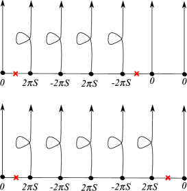
Figure 8: (color online) Two space time configurations differing by the shift of one instanton. The two crosses represent the positions of the singularities. A straight line represents a trivial path in $SO(3)$ while a loop is a non-trivial path. The Berry phase associated with each loop is $\pm 2\pi S$ depending on the sublattice.

For half-integer spins, different instantons-anti-instantons contributions are compensated by destructive interferences. Thus, the two topological sectors $q=0,1$ are non connected and we are left with two degenerate ground states labeled by the two elements of $\pi_{1}(SO(3))$. As shown by Read and Sachdev in a large $N$ analysis of the (2+1)d Heisenberg model SachdevRead1 , this kind of destructive interferences between instantons leads to dimerization in disordered phases. This seems to be the case here: the spin $1/2$ isotropic model is known to be dimerized by DMRG.

On the other hand, integer spins allow instanton events to proliferate as all events come with the same phase. This makes that the two vacua are well connected. This “tunneling” between vacua lifts the degeneracy and the ground state is therefore unique.

V.3 Anisotropic case, $\alpha\neq 1$

For $\alpha\neq 1$, the difference in Berry phase between two matrices $\mathcal{R}$ and $\mathcal{R}+\delta\mathcal{R}$ belonging to the same topological class is:

$$\delta S_{BP}^{\prime} = -iS\int\textrm{d}\tau\;V_{\beta}(\mathcal{R}^{-1}\delta\mathcal{R})_{\beta\beta^{\prime}}\sum_{a}\mathbf{n}_{a\beta^{\prime}}$$ (37)

$$= i\frac{S}{2}\frac{1-\alpha}{\alpha}\int\textrm{d}\tau\;\delta\mathbf{e}_{3}\cdot(\partial_{\tau}\mathbf{e}_{3}\times\mathbf{e}_{3}).$$

In the anisotropic case, the Berry phase can no longer be used to classify topological classes. For example, the path contribution to the partition function from the two configurations drawn on figure 8 is now:

$$Z = ...+\textrm{e}^{2i\pi SL}\left(\textrm{e}^{i\frac{S}{2}\frac{1-\alpha}{\alpha}\int_{0}^{L}\textrm{d}x\int\textrm{d}\tau\;\partial_{x}\mathbf{e}_{3}\cdot(\partial_{\tau}\mathbf{e}_{3}\times\mathbf{e}_{3})}\right.$$

$$+ \left.\textrm{e}^{i2\pi S}\textrm{e}^{i\frac{S}{2}\frac{1-\alpha}{\alpha}\int_{0}^{L+1}\textrm{d}x\int\textrm{d}\tau\;\partial_{x}\mathbf{e}_{3}\cdot(\partial_{\tau}\mathbf{e}_{3}\times\mathbf{e}_{3})}\right)e^{S_{\mathrm{NL\sigma M}}}+...$$

Here, we have been careful to write the total Berry phase as a continuous integral over the string. By doing so, we made the approximation that the order parameter $\mathcal{R}(x,t)$ is sufficiently smooth so that the derivatives $\partial_{x}\mathbf{e}_{i}$ are well-defined. This development is valid if we stay in a given topological sector of $SO(3)$. For a configuration with many instantons, we should separate the contributions from the different topological sectors and write it as a sum of integrals:

$$S_{BP}^{\prime} = i\sum_{i,a}2\pi Sq_{i}(-1)^{i}$$

$$+ i\frac{S}{2}\frac{1-\alpha}{\alpha}\sum_{i=0}^{P-1}\int_{x_{i}}^{x_{i+1}}\textrm{d}x\int\textrm{d}\tau\;\partial_{x}\mathbf{e}_{3}\cdot(\partial_{\tau}\mathbf{e}_{3}\times\mathbf{e}_{3}),$$

where $\{x_{1},\ldots,x_{i}\}$ denotes the position of the $P$ instantons. Note that without instantons (i.e if $\mathcal{R}(x,t)$ is a smooth field everywhere), we can regroup all the integrals into a single one and this term identically vanishes:

$$\int_{-\infty}^{+\infty}\textrm{d}x\int\textrm{d}\tau\;\partial_{x}\mathbf{e}_{3}\cdot(\partial_{\tau}\mathbf{e}_{3}\times\mathbf{e}_{3})$$

$$= \int\int\textrm{d}x\textrm{d}\tau\;\left[\partial_{\tau}(\mathbf{e}_{1}\cdot\partial_{x}\mathbf{e}_{2})-\partial_{x}(\mathbf{e}_{1}\cdot\partial_{\tau}\mathbf{e}_{2})\right]=0,$$

given the periodic boundary conditions we imposed.

Let us finally recover some well-known result in the extreme limits $\alpha=0.5$ and $\alpha\rightarrow\infty$. In this case, the symmetry of the order parameter reduces to $O(3)/O(2)\cong S^{2}$. There are no instantons in this case since $\pi_{1}(S^{2})=1$. It is then straightforward to show that (V.3) reduces to:

$$S_{BP}^{\rm tot\prime}=i\frac{S}{2}\int_{-\infty}^{+\infty}\textrm{d}x\int\textrm{d}\tau\;\partial_{x}\mathbf{e}_{3}\cdot(\partial_{\tau}\mathbf{e}_{3}\times\mathbf{e}_{3})=2i\pi Sn\;n\in\mathbb{Z}$$

We recall that having a non-trivial skyrmion number for a smooth space-time configuration of the vector field $\mathbf{e}_{3}$ requires discontinuities on the field $\mathbf{e}_{1}$. However, as this last field gets zero stiffness for $\alpha=0.5$ and decouples we recover for the field $\mathbf{e}_{3}$ the form of the NL$\sigma$M with the correct topological term of a single chain of spins $S$ as we should.

V.3.1 Half-integer spins

Reiterating the argument that led us to the twofold degeneracy of the ground state for $\alpha=1$ and half-integer spins, we find with (V.3) that the different instantons-anti-instantons contributions do not cancel out anymore. The tunneling process between the two topological sectors is present and the topological degeneracy is lifted. Consequently, we can make use of an important result for spin chains, the Lieb-Schultz-Mattis theorem LSM , suggesting that the system is in a gapless phase. This theorem states that spin Hamiltonians with local interactions and an half-integer spin per unit cell like (1) either support gapless excitations or have a ground-state degeneracy. Ruling out the possibility of a degeneracy here tends to the scenario of a critical behavior. This is indeed what appears in the the study of T. Sakai et al where, for $S=1/2$, the DMRG data point at a preservation of the spin gap only in a narrow range around $\alpha=1$ Sakai .

V.3.2 Integer spins

An interesting application for integer spins is a possible extension of Haldane’s conjecture to the quantum spin tube. Reconsidering again the Berry phase term, we examine the possibility of rewriting the sum of integrals (V.3) into a single one:

$$i\frac{S}{2}\frac{1-\alpha}{\alpha}\sum_{i=0}^{P-1}\int_{x_{i}}^{x_{i+1}}\textrm{d}x\int\textrm{d}\tau\;\partial_{x}\mathbf{e}_{3}\cdot(\partial_{\tau}\mathbf{e}_{3}\times\mathbf{e}_{3})$$

$$\equiv i\frac{S}{2}\frac{1-\alpha}{\alpha}\int_{-\infty}^{+\infty}\textrm{d}x\int\textrm{d}\tau\;\partial_{x}\mathbf{e}_{3}\cdot(\partial_{\tau}\mathbf{e}_{3}\times\mathbf{e}_{3}).$$ (41)

Because of (V.3), we saw that the integral on the right hand side of (41) must vanish for any smooth configuration of the field $\mathcal{R}(x,t)$. However, it is possible that the field $\mathbf{e}_{3}(x,t)$ is smooth but that $\mathcal{R}(x,t)$ is not (see for instance fig 7: the vectors $\mathbf{e}_{1}$ and $\mathbf{e}_{2}$ change sharply of direction where the instantons take place but $\mathbf{e}_{3}$ remains constant). In this case, writing the Berry phase as a single integral is allowed and this integral will be different from zero. However, we must emphasize that the identification (41) is not totally complete, since we elude all the instantons events where $\mathbf{e}_{3}$ is discontinuous. However, in the region $\alpha\sim 0.5$ we saw that in the bare action the stiffness of the $\mathbf{e}_{1}$ is very small. One can then suppose that in this limit the low energy configurations with non-trivial topological index are those where the $\mathbf{e}_{3}$ is smoothly varying and the necessary discontinuities are in the $\mathbf{e}_{1}$ field configuration. Keeping this picture even for larger values of $\alpha$, from (41) one then recognizes a topological term for the unit vector $\mathbf{e}_{3}$. But this time, it is multiplied by a factor $(\alpha-1)/\alpha$. For the $O(3)/O(2)$ NL$\sigma$M, it is known that such a term would lead to a significant change in the spectrum of the model if it is an half-integer, in which case the NL$\sigma$M is gapless. Here, we find $2S$ particular values of $\alpha$ for which this happen:

$$\alpha_{p} = \frac{S}{S-(p+\frac{1}{2})}\rightarrow S_{BP}^{\prime}=i\pi(2p+1)$$

$$-S<p+\frac{1}{2}<S,\;p\in\mathbb{Z},$$

the last inequalities coming from the condition $\alpha>0.5$. For $\alpha=\alpha_{p}$, the Berry phase reduces again to an odd multiple of $\pi$. Finally, the full anisotropic sigma model at these points read:

$$S_{\rm NL\sigma M} = \int\textrm{d}x\textrm{d}\tau\left(\frac{1}{2\tilde{g}_{a}}\left(\tilde{c}_{a}(\partial_{\tau}\mathbf{e}_{a})^{2}+\frac{1}{\tilde{c}_{a}}(\partial_{x}\mathbf{e}_{a})^{2}\right)\right.$$

$$+ \left.\kappa(\mathbf{e}_{3}\cdot\partial_{\tau}\mathbf{e}_{1})^{2}+i\frac{2p+1}{4}\partial_{x}\mathbf{e}_{3}\cdot(\partial_{\tau}\mathbf{e}_{3}\times\mathbf{e}_{3})\right).$$

Would the RG analysis of the preceding section have predicted a decoupling of the field $\mathbf{e}_{1}$, we would have concluded that the last equation represents $2S$ critical field theories, each corresponding to an $SU(2)_{1}$ Wess Zumino Novikov Witten (WZNW) model, as it happens for a dimerized spin $S$ chain Affleck . However, the RG results suggest the opposite scenario: the coupling between the $\mathbf{e}_{1}$ and the $\mathbf{e}_{3}$ is a relevant perturbation and any non-zero skyrmion configuration must come with a fugacity, corresponding to the energy cost of a discontinuity of the $\mathbf{e}_{1}$ field configuration. This would exclude the scenario for a $SU(2)_{1}$ WZNW criticality. Although the one-loop RG results are well suited to study the vicinity of the point $\alpha=1$, one can question their validity in the quasi-collinear regime $\alpha\sim 0.5$. The nature of the transition points $J\to J+1$ ($J$ is the total spin per triangle, see equation (4) is thus unclear for the case $J$ big (i.e. close to $\alpha=0.5$) and we are going now to study the transition $J=0$ to $J=1$ in the case of an $S=1$ tube.

VI The $S=1$ case

In this section, we will focus on the spin-1 case for which two quantum phase transitions are expected (close to $\alpha=1/2$ and $\alpha=2$ respectively when $J_{\parallel}/J_{\perp}\ll 1$).

VI.1 Effective model for the $S=1$ tube

In the small $J_{\parallel}$ limit, we can apply simple perturbation theory in order to obtain an effective model which should be valid close enough to a critical point. As recalled in Sec. II, a single triangle exhibits at low-energy a level crossing between one singlet and one triplet states both at $\alpha=1/2$ and $\alpha=2$. If we restrict ourselves to the neighboring of one level crossing, then we can build an effective model by keeping only these low-lying degrees of freedom. Because the Hilbert space of one singlet plus one triplet is equivalent to two spin 1/2, we prefer to describe the effective model in terms of effective spin 1/2 variables so that the effective model of the spin-tube becomes a spin-1/2 2-leg ladder hamiltonian.

By performing first order (in $J_{\parallel}$) degenerate perturbation, we end up with a SU(2) spin-1/2 ladder that only contains 2-spin exchange interactions of the form :

$$\hat{H}_{\mbox{eff}} = \sum_{i}\tilde{J}_{\perp}\tilde{S}_{i,1}\cdot\tilde{S}_{i,2}+\tilde{J}_{\parallel}(\tilde{S}_{i,1}\cdot\tilde{S}_{i+1,1}+\tilde{S}_{i+1,2}\cdot\tilde{S}_{i+1,2})$$ (44)

$$+ \tilde{J}_{d}\sum_{i}(\tilde{S}_{i,1}\cdot\tilde{S}_{i+1,2}+\tilde{S}_{i+1,2}\cdot\tilde{S}_{i,1})$$

and the effective exchange are as follows:

$$\alpha\simeq 1/2: \quad\tilde{J}_{\perp}=2\alpha-1,\quad\;\tilde{J}_{\parallel}=(\frac{11}{8}+\frac{5}{9})J_{\parallel},$$

$$\tilde{J}_{d}=(\frac{11}{8}-\frac{5}{9})J_{\parallel}\sim 0.82J_{\parallel}.$$ (45)

$$\alpha\simeq 2: \quad\tilde{J}_{\perp}=2-\alpha,\quad\;\tilde{J}_{\parallel}=\frac{13}{9}J_{\parallel},$$

$$\quad\tilde{J}_{d}=\frac{5}{9}J_{\parallel}\sim 0.56J_{\parallel}.$$ (46)

This mapping allows for a straightforward explanation of the occurence of quantum phase transitions. Varying $\alpha$ is equivalent to changing the effective rung exchange from strongly positive to strongly negative, which means that the spin-1/2 ladder is in a rung-singlet phase on one side and in a Haldane phase on the other side. Because this spin-1/2 model is simpler and has already been studied intensively, we can use some results from the literature to clarify the nature of the phase transition.

From the bosonisation point of view, which is valid when $\tilde{J}_{\parallel}$ is the dominant energy scale, Nersesyan and Tsvelik have argued that there should be a transition when $\tilde{J}_{\perp}=2\tilde{J}_{d}$ with the possibility of deconfined spinons Nersesyan2003 . A more refined analysis by Starykh and Balents has shown that marginal interactions modify these conclusions so that the transition between rung singlet and Haldane phase becomes either first order or has an intermediate columnar dimer phase Starykh2004 . These estimates $\tilde{J}_{\perp}=2\tilde{J}_{d}$ for the quantum phase transition are plotted on the phase diagram in Fig. 4.

From the numerical point of view, early DMRG simulations Wang2000 were interpreted in favor of a second order (respectively first order) phase transition for $\tilde{J}_{d}/\tilde{J}_{\parallel}$ smaller (respectively larger) than 0.287. The absence of an intermediate dimerized phase was confirmed by more recent numerical work Hung2006 ; Kim2008 although these studies do not agree on the order of the transition: either it is always first order Kim2008 or it could be continuous for small $\tilde{J}_{d}/\tilde{J}_{\parallel}\sim 0.2$ Hung2006 . Given that our effective models have a relatively large ratio $\tilde{J}_{d}/\tilde{J}_{\parallel}$ (respectively close to 0.42 and 0.38 for both critical cases $\alpha\sim 1/2,2$), all numerical studies agree that the phase transitions are first order.

VI.2 DMRG results for the $S=1$ tube

In order to have an unbiased answer, we have decided to perform numerical simulations of the $S=1$ tube with the powerful DMRG algorithm dmrg for several values of $J_{\parallel}$. Simulations are done mostly with open boundary conditions (OBC) with system sizes up to $3\times 64$, but also with periodic boundary conditions (PBC) on some cases. Typically, we keep up to 1600 states, which is sufficient to have a discarded weight smaller than $10^{-8}$.

VI.2.1 String order parameter

In order to draw a numerical phase diagram and to compare it with the conjectured one (see Fig. 4), we have computed the $z$-component of the string order parameter (see Eq. (9)) for several values of $J_{\parallel}$ and $\alpha$. In order to extract the bulk value and avoid finite-size effects due to the edges, we have taken the following definition in our simulations:

$$\left\langle\mathcal{O}^{z}\right\rangle=\left\langle J^{z}_{L/4}\exp\left(i\pi\sum_{l=L/4}^{3L/4}J_{l}^{z}\right)J^{z}_{3L/4+1}\right\rangle$$ (47)

In Fig. 9, we plot this quantity as a function of the frustration $\alpha$ for a small $J_{\parallel}/J_{\perp}=0.1$. We conclude that the string order is finite for $\alpha<0.57$ and $\alpha>1.92$, and it vanishes elsewhere, i.e. our model does exhibit quantum phase transitions. Therefore, as a function of $\alpha$, we find successively a topological phase (with $S_{b}=1/2$ in the presence of OBC), a non-topological one, and again a topological phase (with $S_{b}=1/2$ in the presence of OBC). This is the behaviour expected from the perturbation and the mapping to an effective spin-1 or spin-0 chain. Indeed, for small or large $\alpha$, we can derive an effective spin-1 Haldane model for which the string order parameter is known white93 to be $\sim 0.374$, which is close to our value in both limits.

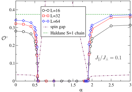
Figure 9: (color online) String order parameter along $z$ of the spin-1 tube as a function of the anisotropy parameter for $J_{\parallel}=0.1J_{\perp}$ and various lengths $L$. The extrapolated spin gap (see Fig. 13 below) is also shown, as well as the non-local order parameter of the spin-1 Haldane chain.

In order to complete our phase diagram in Fig. 4, we also compute the string order parameter for larger $J_{\parallel}/J_{\perp}$ where perturbation is no more valid. Data are shown in Fig. 10 and have a quite different behaviour: now, the string order parameter is finite for all $\alpha$, i.e. we have no phase transitions along this line.

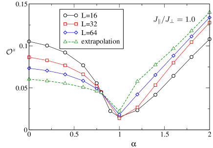
Figure 10: (color online) String order parameter along $z$ of the spin-1 tube as a function of the anisotropy parameter for $J_{\parallel}=J_{\perp}$ and various lengths $L$. A linear extrapolation with the largest sizes is also plotted and is finite for all $\alpha$.

By computing $\langle\mathcal{O}^{z}\rangle$ for various $J_{\parallel}$ and $\alpha$, we estimate that the tip of the $J=0$ lobe occurs for $J_{\parallel}/J_{\perp}=0.67$ and $\alpha=1$.

Now, we present data for a vertical cut in the phase diagram of Fig. 4 by fixing $\alpha=0.75$. By varying $J_{\parallel}/J_{\perp}$, the string order plotted in Fig. 11 vanishes for $J_{\parallel}/J_{\perp}\leq 0.34$ and is finite beyond. In Fig. 11, the string order parameter $\langle\mathcal{O}^{z}\rangle$ remains finite up to $J_{\parallel}/J_{\perp}\sim 3$. However, as we have discussed in Sec. III.3, $\langle\mathcal{O}^{z}\rangle$ vanishes in the weak coupling limit.

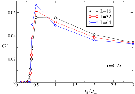
Figure 11: (color online) String order parameter along $z$ of the spin-1 tube as a function of $J_{\parallel}/J_{\perp}$ for a fixed anisotropy parameter $\alpha=0.75$ and various sizes.

In order to ascertain that there is no other phase transition when going to the decoupled chain limit, we have computed the product string order parameter of Eq. (16) as well as the usual one for the non-frustrated case $\alpha=0$. Data are shown in Fig. 12 for both order parameters. When the chains are almost decoupled, the product string order parameter is close to the product of the standard string order parameter for the independent chains. On the opposite side, when the dominant coupling is $J_{\perp}$, the perturbative argument that we have given above (see Sec. VI.1) indicates that the 3-leg ladder behaves effectively as a spin-1 chain for which the string order parameter $\langle\mathcal{O}^{z}\rangle$ reduces to the usual one; this is indeed what is found numerically on large system size.

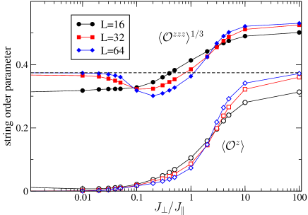
Figure 12: (color online) Various string order parameters of the spin-1 ladder ($\alpha=0$) as a function of $J_{\perp}/J_{\parallel}$ for various sizes. Usual (respectively product) string order along $z$ is shown with open (respectively filled) symbols. The dashed line indicates the known value for the spin-1 Haldane chain white93 .

VI.2.2 Spectral gap

We have also calculated the excitation gap by DMRG. In order to estimate the bulk gap, the gap is extracted differently from the finite-size spectrum depending on the boundary conditions. For open boundary conditions (OBC), in a Haldane-like phase, the real gap should be calculated between the $S=1$ sector and the $S=2$ sector since the sectors $S=0$ and $S=1$ are already degenerate because of the edge states. On the contrary, for a singlet-like state, the gap is defined between the $S=0$ sector and the $S=1$ sector. For periodic boundary conditions, there are no edge states and thus, the gap is uniquely defined to be between $S=0$ and $S=1$. The evolution of the gap is presented on Figure 13 (left for OBC and right for PBC). For OBC on largest system sizes and fixed $J_{\parallel}/J_{\perp}=0.1$, the DMRG indicates that the gap between $S=0$ and $S=1$ is almost zero for $\alpha<0.57$ or $\alpha>1.92$ but is finite in between (data not shown). The gap between $S=1$ and $S=2$ is plotted on Fig. 13 for $J_{\parallel}=0.1J_{\perp}$ and exhibits a striking difference in three regions. For $\alpha<0.57$ or $\alpha>1.92$, the gap is finite and almost constant with $\alpha$. In contrast, in the intermediate $\alpha$ region, the gap increases almost linearly away from these critical points. Extrapolation of the data for large system sizes seems to go in favor of a finite gap everywhere (see Fig. 13), but note that the extrapolated gap at the critical points is extremely small. Both critical points are identical to the values we had found with the string order parameter. We observe that the gap is roughly constant in the $S_{b}=1/2$ phase, except in the vicinity of the transition point. Note that this is in accordance with the qualitative picture of the strong coupling limit. For small or very large $\alpha$, the effective model is a spin-1 chain with an effective spin exchange of order $J_{\parallel}$ (but independent of $\alpha$); therefore, the spin gap essentially depends on the value of $J_{\parallel}$ but is independent of the anisotropy parameter $\alpha$.

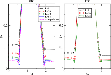
Figure 13: (color online) Spin gap of the spin-1 tube as a function of the anisotropy parameter. $J_{\parallel}=0.1J_{\perp}$ and both open and periodic boundary conditions (OBC/PBC) are considered.

In order to make connection with the perturbation theory, we have also performed simulations of the effective spin-1/2 ladder (see Eq. (44)) corresponding to our parameters choice. Due to the Hilbert space reduction, we are able to simulate larger clusters. As can be seen on Fig. 14, we obtain a very good agreement between both sets of data since we are indeed considering a small $J_{\parallel}$ case where perturbation is expected to be accurate. We have plotted an infinite-size extrapolation by using the two biggest ladders ($L=64$ and $L=128$) which confirm that the spin gap has a large drop around $\alpha=0.57$. However, at the critical point, the spin gap does not vanish and our data suggest an extremely small but finite value. This result would indicate a first-order phase transition, in agreement with other numerical studies on the ladder systems Wang2000 ; Hung2006 ; Kim2008 .

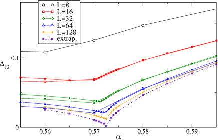
Figure 14: (color online) Spin gap of the spin-1 tube as a function of the anisotropy parameter (open symbols) or of the effective 2-leg spin-1/2 ladder (filled symbols). $J_{\parallel}=0.1J_{\perp}$ and open boundary conditions are used. The infinite-size extrapolation was performed with the two largest ladder clusters.

VI.2.3 Von Neumann entropy

In this part, we fix $J_{\parallel}/J_{\perp}=0.1$ for which we have found two quantum phase transitions for $\alpha=0.57$ and $\alpha=1.92$, both with an extremely small but finite spin gap at the transition. Since these critical points seem to be very close to tricritical points (the correlation lengths are very large at the transitions), another quantity of interest here is the von Neumann entropy of a finite segment of the chain. It is defined by:

$$S_{vN}(\ell)=-\textrm{Tr}(\rho_{\ell}\ln\rho_{\ell})$$ (48)

where $\rho_{\ell}=\textrm{Tr}_{\ell}\rho$ is the reduced density matrix associated to a block of $\ell$ spins. This quantity is known to behave fundamentally differently for critical and non-critical systems Vidal ; Cardy . It saturates at a finite value when the system is non critical while it increases logarithmically for critical systems. The analytic expression of $S_{\ell}$ is given by:

$$S_{vN}(\ell)=\frac{c}{6}\ln\left[\frac{2L}{\pi}\sin\left(\frac{\pi\ell}{L}\right)\right]+g$$ (49)

where $c$ is the central charge, and $g$ is a constant. The Von Neumann entropy is represented on Figure 15 as a function of the conformal distance $d(\ell)=\sin(\pi\ell/L)$. For $\alpha=0.5$ and $\alpha=0.6$, the entropy converges to a finite value (the same results holds for all other values far enough from both critical points). On the contrary, for $\alpha=0.57$ and $\alpha=1.92$, it does not saturate but grows with the system size, which should be in favor of a gapless character of the two critical points. The entropy displays also a large periodic oscillation. Such an oscillation has already been observed in other critical spin chains Laflo2006 and may be related to the existence of soft modes at $k=0$ and $k=\pi$ in the problem Legeza . Thus, the decay in correlation function would not be simply algebraic at the critical point but the decaying function would be multiplied by an oscillatory factor. Because of the oscillations, it is hard to distinguish what is the best fit between $c=\frac{3}{2}$ and $c=2$.

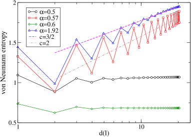
Figure 15: (color online) Plot of the Von Neumann entropy as a function of $d(\ell)$ for different values of the anisotropy parameter and fixed $J_{\parallel}=0.1J_{\perp}$.

However, from our DMRG data on the gap, as well as the mapping to an effective ladder, we conclude to a very weak first-order transition, especially in the strong coupling limit $J_{\parallel}\ll J_{\perp}$. This last scenario is supported by the bosonisation studies and the DMRG simulation of the effective Hamiltonian (44). Still, von Neumann entropy exhibits a critical behaviour with $c=3/2$ or $c=2$ at the critical points, which is valid on rather large length scales. Therefore, we believe that this spin tube can be tuned very close to a tricritical point separating a first-order transition line from a possible continuous transition line nearby. The gapless transition at the critical points could then be correlated with the presence of a non trivial topological term in the NL$\sigma$M. Note that there are no such critical points in the phase diagram of the two-leg ladder with $S=1$ Todo ; Allen2000 , and that there is no topological term in the corresponding NL$\sigma$M as well Senechal2 . Of course, the link between the NL$\sigma$M and the critical point of the DMRG data still needs to be clarified with further investigations, both analytically and numerically.

VII The $S=2$ case

In this section, we consider the spin-2 case for which four quantum phase transitions are expected as a function of the frustration $\alpha$ for a fixed $J_{\parallel}/J_{\perp}\ll 1$.

VII.1 Effective model for the $S=2$ tube

In principle, one can apply simple perturbation theory in order to obtain an effective model valid close enough to any of the critical points for small $J_{\parallel}/J_{\perp}$. Here, we have two types of critical points: (i) close to $\alpha=1/2$ or $\alpha=3$, and as recalled in Sec. II, a single triangle will have a quintet and a triplet as low-energy states; (ii) close to $\alpha=2/3$ or $\alpha=3/2$, low-energy states consist in one triplet and one singlet.

Although one can derive both kinds of effective models, case (i) does not allow to make analytical progress. On the contrary, for the second case, the effective model turns out to be formally the same as for the spin-1 tube (see part VI.1), i.e. first-order degenerate perturbation results can be mapped onto a SU(2) spin-1/2 ladder that only contains 2-spin exchange interactions of the form given in Eq. (44). The effective exchanges are given as:

$$\alpha \simeq 2/3:\quad\tilde{J}_{\perp}=3\alpha-2,\quad\;\tilde{J}_{\parallel}=\frac{23}{5}J_{\parallel},$$ (50)

$$\tilde{J}_{d}=\frac{7}{5}J_{\parallel}.$$

$$\alpha \simeq 3/2:\quad\tilde{J}_{\perp}=3-2\alpha,\quad\;\tilde{J}_{\parallel}=\frac{151}{40}J_{\parallel},\quad\tilde{J}_{d}=\frac{39}{40}J_{\parallel}.$$

As explained in details in part VI.1, such a mapping explains the occurence of a quantum phase transition when $\tilde{J}_{\perp}\simeq 2\tilde{J}_{d}$, as well as giving insight on the order of the transition.

Both quantum critical lines are plotted in Fig. 5. Moreover, for both cases we are in a regime where $\tilde{J}_{d}/\tilde{J}_{x}\sim 0.25-0.30$, for which there is no consensus yet on the order of the transition Hung2006 ; Kim2008 . Still, if the transitions are first-order, the gap at the transition should be very small, which means that for most practical purpose, the system will appear critical on length scales smaller than the (large) correlation length.

VII.2 DMRG results for the spin $S=2$ tube

Simulations are done mostly with open boundary conditions (OBC) with system sizes up to $3\times 64$, but also with periodic boundary conditions (PBC) on some cases. Typically, we keep up to 1600 states, which is sufficient to have a discarded weight smaller than $10^{-6}$.

We have computed several spectral gaps with various boundary conditions and various total spin sector, in order to avoid edge effects, but finite-size effects are rather large and spin gap values quite small so that no definite answer on the phase diagram can be obtained this way.

A clearer signal is given by the string order parameter (see Eq. 47) which can distinguish between odd-$J$ and even-$J$ Haldane phases. Unfortunately, this quantity alone cannot distinguish between $J=0$ and $J=2$ phase but we can rely on the presence/absence of edge states to distinguish these phases. In Fig. 16, we plot various spin gaps as a function of the frustration $\alpha$. Obviously, if edge states carry a spin $S_{b}$, then the bulk spin gap is obtained between lowest levels of total spin $(2S_{b})$ and $(2S_{b}+1)$, $\Delta_{2S_{b},2S_{b}+1}$, i.e. once edge states have been polarized. In the thermodynamic limit, the two $S_{b}$ edge states form $(2S_{b}+1)^{2}$ degenerate states. Our data are obtained on finite lengths up to $L=32$ and we perform a $1/L$ linear extrapolation to get an estimate of the thermodynamic limit spin gaps. For a small $J_{\parallel}/J_{\perp}=0.1$, our data shown in Fig. 16 indicate successively regions with $S_{b}=1$, $1/2$, $0$ and then in reverse order for increasing $\alpha$, as had been conjectured initially in section III.2.

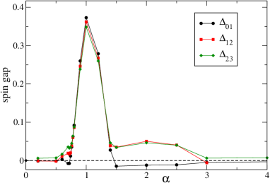
Figure 16: (color online) Various spin gaps $\Delta_{ab}$ for the spin-2 tube as a function of $\alpha$ for $J_{\parallel}/J_{\perp}=0.1$. Data are extrapolated to the thermodynamic limit from simulations with systems of length $L=8$, $16$, and $32$.

In order to get more insight in this phase diagram, we have computed the string order parameter (see Eq. 47) for several exchange couplings. Data are shown in Fig. 17 and confirm the existence of even/odd Haldane S phases: a spin 0 phase has a vanishing order parameter already on finite systems (see $\alpha$ close to 1); a spin 1 phase has a finite and positive string order parameter; a spin 2 phase should have a zero string order parameter but the finite-size scaling is rather slow, as is already known for the spin-2 Haldane chain for instance Yamamoto1997 . Note that the string order data are perfectly consistent with the edge states picture drawn from the spin gap data. This way, one can draw a quantitative phase diagram for the spin 2 tube in Fig. 18, which confirms the qualitative picture conjectured in Fig. 5.

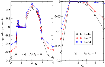
Figure 17: (color online) String order for the spin-2 tube as a function of $\alpha$ for various lengths $L$ with (a) $J_{\parallel}/J_{\perp}=0.1$ or (b) $J_{\parallel}/J_{\perp}=1$.

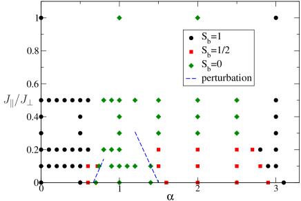
Figure 18: (color online) Numerical phase diagram for the spin-2 tube obtained from the spin gap and the string order parameter.

VIII Discussion and Conclusion

In this paper we have shown that a simple model such as a three-leg quantum spin ladder can give rise to a very rich phase diagram. As it is now ubiquitous in quantum spin chains, integer and half integer spin must be treated separately. For half-integer spins, the Berry phase analysis of Section V.3.1 points towards a quantum phase transition between a gapped spectrum and a degenerate ground state for $\alpha$ close to $1$ and a gapless regime on each side of this phase, as it has indeed being observed for the $S=1/2$ case Sakai . The semiclassical picture of this scenario is a phase transition separating a gapped isotropic coplanar phase and a pseudo-collinear gapless regime. Not surprisingly the difference in behavior at large scales is dictated by the Berry phase terms present in the action.

For integer spins the situation is even more interesting. If we consider the strong coupling regime $J_{\perp}\gg J_{\parallel}$ it makes no doubt that $2S$ quantum phase transitions are expected for a spin $S$ tube when varying the anisotropy parameter $\alpha$. These phase transitions separate gapped phases, and this scenario is reminiscent of what happens in dimerized spin chains when varying the dimerization parameter (see for example I. Affleck’s lectures Affleck ).

These phase transitions can be understood in terms of spontaneous breaking of the hidden $\mathbb{Z}_{2}\times\mathbb{Z}_{2}$ symmetry. The broken hidden $\mathbb{Z}_{2}\times\mathbb{Z}_{2}$ symmetry can be detected by a string order parameter or by edge states with half-integer spin. While a simple generalization of the string order parameter to the tube vanishes in the weak rung coupling limit, an alternative string order parameter remains finite in the same limit for odd spin $S$. Additionally, in some regions of the phase diagram, there exist “phases” with integer-spin edge states. Although they appear to be non-trivial phases, they can be adiabatically connected to a trivial phase with no edge state. This is consistent with an unbroken hidden $\mathbb{Z}_{2}\times\mathbb{Z}_{2}$ symmetry in these “phases”.

More insight into the phase diagram can be obtained with the recent discussion concerning the characterization of the Haldane phase GuWen ; Pollmann09a ; Pollmann09b . The Haldane phase can remain a distinct phase separated from a trivial phase by a quantum phase transition, even when the hidden $\mathbb{Z}_{2}\times\mathbb{Z}_{2}$ symmetry is not well-defined and the string order parameter is not useful. It turns out that the Haldane phase is a topological phase protected by any one of the following three symmetries: 1) global D₂ ($=$ $\mathbb{Z}_{2}\times\mathbb{Z}_{2}$) symmetry of $\pi$-rotation about $x,y$ and $z$ axes, 2) time-reversal symmetry (for $\vec{S}_{j}\rightarrow-\vec{S}_{j}$), and 3) lattice inversion symmetry about a bond center (link parity). The hidden $\mathbb{Z}_{2}\times\mathbb{Z}_{2}$ symmetry is well-defined only with the symmetry 1) above. Most generally, the Haldane phase is characterized by an exact double degeneracy of the entanglement spectrum.

In this paper, we limited our discussion to the tube with SU(2) symmetry of spin rotation and all the symmetries 1)–3) listed above. Within this limitation, the hidden $\mathbb{Z}_{2}\times\mathbb{Z}_{2}$ symmetry can be used to characterize the nontrivial phases, which have edge states with a half-integer spin $S_{b}$. On the other hand, we expect that the phases with the broken hidden $\mathbb{Z}_{2}\times\mathbb{Z}_{2}$ symmetry correspond to the generalized Haldane phase with an exact double degeneracy of the entanglement spectrum. It is protected by either of the symmetries 2) or 3), even when the symmetry 1) is explicitly broken and the hidden $\mathbb{Z}_{2}\times\mathbb{Z}_{2}$ symmetry is ill-defined. In particular, as long as the lattice inversion symmetry abount a bond center is preserved, the generalized Haldane phase is protected as a distinct topological phase. This protection may be roughly understood by the intrinsic odd parity with respect to the lattice inversion associated to an odd number of valence bonds between the neighboring rungs Pollmann09a .

The above general analysis implies the existence of a quantum phase transition between a “topological” phase and a “trivial” phase. However, it does not tell the order of the transition or its universality class.

For dimerized chains, the NL$\sigma$M approach shows that the critical points correspond to an effective half-integer chain which is described by an $SU(2)_{1}$ WZNW model. Our analysis of the NL$\sigma$M in the triangular spin tube has shown that the situation is different here indicating that we must expect phase transition of a different kind. Arises then the question of whether these transition points are expected to be first order or more interesting critical theories as for example higher levels $SU(2)$ WZNW models.

The case of the $S=1$ ladder has proven to be a very interesting and instructive example. The low energy behavior of this system can be shown to be equivalent to a two-leg spin $1/2$ ladder. This ladder system has two obvious extreme regimes corresponding to a collection of singlet states (strong antiferromagnetic couplings between the chains) and a Haldane phase of an effective spin $1$ chain (strong ferromagnetic coupling between the chains). The most recent bosonization analysis Starykh2004 indicates that the transition between these two regimes can be either first order, or a couple of (gapless) lines surrounding a dimerized phase. These gapless lines have central charges $c=1/2$ and $c=3/2$, this last one corresponding to a $SU(2)_{2}$ WZNW model. We have performed extensive DMRG computations on this system. The analysis of the spectral gap and the von Neumann entropy tend to indicate a weak first order transition for our system, but in any case the close proximity to the tricritical point. This allows us to speculate that by introducing further microscopic parameters, as for example second neighbors interactions, the transition can be made second order, but this issue is beyond the scope of the present work. This result is also encouraging for analyzing the nature of the transition for higher spins with both numerical and novel analytical techniques.

One important point is that many of the results obtained here generalize to ladders with a higher odd number of legs displayed with periodic boundary conditions (so in a frustrating manner). Of course frustration becomes weaker as one increase the number of legs. In this sense the 3-leg ladder is a representative of a family of quasi one-dimensional systems where frustration plays a crucial role in the emergence of an interesting physics.

- (1) F. D. M. Haldane, Phys. Rev. Lett. 50, 1153 (1983).
- (2) S. R. White, Phys. Rev. B 53, 52 (1996); E. H. Kim, G. Fáth, J. Sólyom, and D. J. Scalapino, Phys. Rev. B 62, 14965 (2000).
- (3) O. A. Starykh and L. Balents, Phys. Rev. Lett. 93, 127202 (2004).
- (4) E.H. Kim, Ö. Legeza and J. Sólyom, Phys. Rev. B 77, 205121 (2008).
- (5) I. Affleck, T. Kennedy, E. H. Lieb, and H. Tasaki, Phys. Rev. Lett. 59, 799 (1987); Commun. Math. Phys. 115, 477 (1988).
- (6) M. den Nijs and K. Rommelse, Phys Rev. B textbf40, 4709 (1989).
- (7) T. Kennedy, J. Phys. Condens. Matter 2, 5737 (1990); K. Chang, I. Affleck, G. W. Hayden, and Z. G. Soos, J. Phys. Condens. Matter 1, 153 (1989), U. Schollwöck, T. Jolicoeur, and T. Garel, Phys. Rev. B 53, 3304 (1996).
- (8) H. Tasaki, Phys. Rev. Lett. 66, 798 (1991).
- (9) T. Kennedy and H. Tasaki, Phys. Rev. B 45, 304 (1992).
- (10) S. Todo, M. Matsumoto, C. Yasuda, and H. Takayama, Phys. Rev. B 64, 224412 (2001).
- (11) F. Anfuso and A. Rosch, Phys. Rev. B 76, 085124 (2007).
- (12) A. Kolezhuk, R. Roth, and U. Schollwöck, Phys. Rev. Lett. 77, 5142 (1996).
- (13) H. J. Schulz, Correlated Fermions and Transport in Mesoscopic Systems, edited by T. MArtin, G. Montambaux and T. Trân Thanh Vân, Frontiers, Gif-sur-Yvette, France (1996).
- (14) T. Sakai et al.,Phys. Rev. B 78, 184415 (2008).
- (15) G. Sierra, J. Phys. A: Math. Gen 69, 3299 (1996).
- (16) P. Azaria, B. Delamotte, F. Delduc, and Th. Jolicoeur, Nucl. Phys. B 408, 485 (1993).
- (17) T. Dombre and N. Read, Phys. Rev. B 39, 6797 (1989).
- (18) P. Azaria, B. Delamotte, and D. Mouhanna, Phys. Rev. Lett, 68, 1762 (1992).
- (19) F. D. M. Haldane, Phys. Rev. Lett. 61, 1029 (1988).
- (20) S. Rao and D. Sen, Nucl. Phys. B 424, 547 (1994); J. Phys. Condens. Matter 9, 1831 (1997).
- (21) Z.-C. Gu and X.-G. Wen, Phys. Rev. B 80, 155131 (2009).
- (22) F. Pollmann, E. Berg, A. M. Turner, and M. Oshikawa, preprint arXiv0909.4059v1.
- (23) M. Oshikawa, J. Phys. Condens. Matter. 4, 7469 (1992).
- (24) E. Berg, E. G. Dalla Torre, T. Giamarchi, and E. Altman, Phys. Rev. B 77, 245119 (2008).
- (25) J. B. Kogut, Rev. Mod. Phys. 51, 659 (1979).
- (26) See also E. Manousakis, Rev. Mod. Phys. 63, 1 (1991).
- (27) S. Chakravarty, B. Halperin and D. Nelson, Phys. rev. Lett. 60, 1057 (1988).
- (28) T. Einarsson and H. Johannesson, Phys. Rev. B 43, 5867 (1991).
- (29) E. Fradkin, Field Theories in Condensed Matter, Addison Wesley Publishing Company (1991).
- (30) D. Mouhanna, PhD Thesis, Université de Paris VI.
- (31) We have compared the velocities deduced from the NLM and the one obtained from a spin-wave expansion at leading order. It appears that the values of and slightly differs in the two approaches away from . This might be due to the difference between Eq. (19) and Eq. (IV.2). However, we find that the result of the integration of the RG equations is not altered by these variations.
- (32) A. M. Polyakov, Nucl. Phys. B 120, 429 (1977); Gauge fields and strings, Harwood Academic Publishers (1987).
- (33) S. Nishimoto and M. Arikawa, Phys. Rev. B 78, 054421 (2008).
- (34) C. K. Majumdar and D. K. Gosh, J. Math. Phys. 10, 1388 (1969).
- (35) N.D. Mermin, Rev. Mod. Phys. 51, 591 (1979).
- (36) H. Kawamura and S. Miyashita, J. Phys. Soc. Jpn. 53, 9 (1984).
- (37) N. Read and S. Sachdev, Phys. Rev. B 42, 4568 (1990).
- (38) E. H. Lieb, T. D. Schultz, and D. C. Mattis, Ann. Phys. (N.Y.) 16, 407 (1961).
- (39) I. Affleck, Field theory methods and quantum critical phenomena, in Les Houches, session XLIX, Champs, Cordes et Phénomèmes critiques (Elsevier, New-York, 1989).
- (40) A. A. Nersesyan and A. M. Tsvelik, Phys. Rev. B 67, 024422 (2003).
- (41) X. Wang, Mod. Phys. Lett. B 14, 327 (2000).
- (42) H.-H. Hung, C.-D. Gong, Y.-C. Chen, and M.-F. Yang, Phys. Rev. B 73, 224433 (2006).
- (43) S. R. White, Phys. Rev. Lett. 69, 2863 (1992).
- (44) S. R. White and D. A. Huse, Phys. Rev. B 48, 3844 (1993).
- (45) G. Vidal, J. I. Latorre, E. Rico, and A. Kitaev, Phys. Rev. Lett. 90, 227902 (2003).
- (46) P. Calabrese and J. Cardy, J. Stat. Mech. 06 P06002 (2004).
- (47) N. Laflorencie, E. S. Sørensen, M.-S. Chang, and I. Affleck, Phys. Rev. Lett. 96, 100603 (2006).
- (48) Ö. Legeza, J. Sólyom, L. Tincani, and R.M. Noack, Phys. Rev. Lett. 99, 087203 (2007).
- (49) D. Allen and D. Sénéchal, Phys. Rev. B 61, 12134 (2000).
- (50) D. Sénéchal, Phys. Rev. B 52, 15319 (1995).
- (51) S. Yamamoto, Phys. Rev. B 55, 3603 (1997).
- (52) F. Pollmann, A. M. Turner, E. Berg, and M. Oshikawa, Phys. Rev. B 81, 064439 (2010).