Key Generation in Wireless Sensor Networks
Based on Frequency-selective Channels –
Design, Implementation, and Analysis

Abstract

Key management in wireless sensor networks faces several new challenges. The scale, resource limitations, and new threats such as node capture necessitate the use of an on-line key generation by the nodes themselves. However, the cost of such schemes is high since their secrecy is based on computational complexity. Recently, several research contributions justified that the wireless channel itself can be used to generate information-theoretic secure keys. By exchanging sampling messages during movement, a bit string can be derived that is only known to the involved entities. Yet, movement is not the only possibility to generate randomness. The channel response is also strongly dependent on the frequency of the transmitted signal. In our work, we introduce a protocol for key generation based on the frequency-selectivity of channel fading. The practical advantage of this approach is that we do not require node movement. Thus, the frequent case of a sensor network with static motes is supported. Furthermore, the error correction property of the protocol mitigates the effects of measurement errors and other temporal effects, giving rise to an agreement rate of over 97 %. We show the applicability of our protocol by implementing it on MICAz motes, and evaluate its robustness and secrecy through experiments and analysis.

1 Introduction

Securing wireless sensor networks (WSNs) has been one of the main wireless network research areas in recent years. Especially key generation and key management, which are at the heart of any security design, pose new challenges because of the low computational capabilities of wireless motes, their limited battery lifetime, and the broadcast nature of wireless communication. Given these peculiarities, a large number of key management protocols for WSNs has been proposed, often fine-tuned between different performance vs. security trade-offs and adapted for specific WSN scenarios and their applications (for a general overview see, e.g., [6, 31]). However, most of these protocols follow a conventional cryptographic approach, where the secret is based either on pre-distributed keys or public-key schemes assuming more performance capable devices that are able to generate and distribute the keys. Although there have been efforts to adapt public key cryptographic protocols to the world of WSNs (e.g., TinyECC [14]), these adaptations usually have a significant complexity and memory footprint as well as a high energy consumption (for energy analysis of public key schemes, see, e.g., [27]). As an example, TinyECC (with optimizations) requires roughly 20 kB of ROM and 1.7 kB of RAM [14], which is 15.6 % and 42.5 % of the overall available memory resources of MICAz sensor motes, respectively, and single operations require computation time in the order of seconds.

Recently, there have been research contributions that follow an alternative path towards key generation using an information-theoretic approach to derive secrets from unauthenticated broadcast channels. Informally, the general idea is similar to the quantum world, in which the laws of quantum mechanics ensure that two spatially separated particles experience highly correlated quantum states (called “quantum entanglement”). Measuring the quantum properties of one particle discloses the knowledge of another. However, in contrast to the mystical quantum nature, contributions on key generation using wireless channel are concerned with conventional physical signal propagation and, to some extent, its reciprocal behavior. Specifically, recent results described by Mathur et al. [15] and Azimi-Sadjadi et al. [2] justify that the unpredictable multipath propagation and the resulting fading behavior of wireless channel can be used to extract shared secret material. Simply by exchanging messages that serve to sample the signal propagation behavior, both transmitters can establish mutual secret information, while an eavesdropper who also receives these messages still remains completely ignorant of their channel measurements. Since the secrecy of the extracted information is not based on computational complexity as common to conventional public key cryptography, these protocols are especially valuable to computationally limited wireless devices. Yet, existing solutions require that the wireless devices move at certain speeds to produce enough unpredictability in their signals. Thus, the most prevalent applications of WSNs which are based on static wireless motes make these protocols inapplicable. This brings us to the contribution of this work, which abstains from this limitation and provides a novel key generation protocol for static WSNs. The main contributions of this paper are:

• Design of a robust key generation protocol with an error-correcting property against channel deviations ($\rightarrow$ Section 4).

• Implementation of the protocol on static MICAz sensor motes and analysis of the protocol’s robustness and the secrecy of derived keys, especially with respect to dependencies between wireless channels ($\rightarrow$ Section 5).

• Derivation of a stochastic model describing the secrecy of the protocol, its validation using experimental data, and guidelines on increasing the number of generated secret bits ($\rightarrow$ Section 6).

In summary, we demonstrate the applicability of a key generation protocol that takes advantage of the wireless channel behavior in static wireless networks and analyze different trade-offs between it’s robustness to channel deviations and available secrecy.

2 Related Work

\psfrag{Wireless channels}{\footnotesize{Wireless channels}}\psfrag{Received signal strength [dBm]}{\footnotesize{Received signal strength (dBm)}}\psfrag{11}[1][0]{\tiny{$11$}}\psfrag{12}[1][0]{\tiny{$12$}}\psfrag{13}[1][0]{\tiny{$13$}}\psfrag{14}[1][0]{\tiny{$14$}}\psfrag{15}[1][0]{\tiny{$15$}}\psfrag{16}[1][0]{\tiny{$16$}}\psfrag{17}[1][0]{\tiny{$17$}}\psfrag{18}[1][0]{\tiny{$18$}}\psfrag{19}[1][0]{\tiny{$19$}}\psfrag{20}[1][0]{\tiny{$20$}}\psfrag{21}[1][0]{\tiny{$21$}}\psfrag{22}[1][0]{\tiny{$22$}}\psfrag{23}[1][0]{\tiny{$23$}}\psfrag{24}[1][0]{\tiny{$24$}}\psfrag{25}[1][0]{\tiny{$25$}}\psfrag{26}[1][0]{\tiny{$26$}}\psfrag{-50}[1][0]{\tiny{-$50$}}\psfrag{-60}[1][0]{\tiny{-$60$}}\psfrag{-70}[1][0]{\tiny{-$70$}}\psfrag{-80}[1][0]{\tiny{-$80$}}\psfrag{-90}[1][0]{\tiny{-$90$}}\psfrag{-55}[1][0]{\tiny{-$55$}}\psfrag{-65}[1][0]{\tiny{-$65$}}\psfrag{-75}[1][0]{\tiny{-$75$}}\psfrag{-85}[1][0]{\tiny{-$85$}}\psfrag{-95}[1][0]{\tiny{-$95$}}\includegraphics[width=134.42113pt]{figures/rss-barplot/eps/CircleSem-00-Alice}

(a) Alice’s view when Bob transmits

\psfrag{Wireless channels}{\footnotesize{Wireless channels}}\psfrag{Received signal strength [dBm]}{\footnotesize{Received signal strength (dBm)}}\psfrag{11}[1][0]{\tiny{$11$}}\psfrag{12}[1][0]{\tiny{$12$}}\psfrag{13}[1][0]{\tiny{$13$}}\psfrag{14}[1][0]{\tiny{$14$}}\psfrag{15}[1][0]{\tiny{$15$}}\psfrag{16}[1][0]{\tiny{$16$}}\psfrag{17}[1][0]{\tiny{$17$}}\psfrag{18}[1][0]{\tiny{$18$}}\psfrag{19}[1][0]{\tiny{$19$}}\psfrag{20}[1][0]{\tiny{$20$}}\psfrag{21}[1][0]{\tiny{$21$}}\psfrag{22}[1][0]{\tiny{$22$}}\psfrag{23}[1][0]{\tiny{$23$}}\psfrag{24}[1][0]{\tiny{$24$}}\psfrag{25}[1][0]{\tiny{$25$}}\psfrag{26}[1][0]{\tiny{$26$}}\psfrag{-50}[1][0]{\tiny{-$50$}}\psfrag{-60}[1][0]{\tiny{-$60$}}\psfrag{-70}[1][0]{\tiny{-$70$}}\psfrag{-80}[1][0]{\tiny{-$80$}}\psfrag{-90}[1][0]{\tiny{-$90$}}\psfrag{-55}[1][0]{\tiny{-$55$}}\psfrag{-65}[1][0]{\tiny{-$65$}}\psfrag{-75}[1][0]{\tiny{-$75$}}\psfrag{-85}[1][0]{\tiny{-$85$}}\psfrag{-95}[1][0]{\tiny{-$95$}}\includegraphics[width=134.42113pt]{figures/rss-barplot/eps/CircleSem-00-Bob}

(b) Bob’s view when Alice transmits

\psfrag{-5.5}[1][0]{\tiny{-$5.5$}}\psfrag{-5}[1][0]{\tiny{-$5$}}\psfrag{-4.5}[1][0]{\tiny{-$4.5$}}\psfrag{-4}[1][0]{\tiny{-$4$}}\psfrag{-3.5}[1][0]{\tiny{-$3.5$}}\psfrag{-3}[1][0]{\tiny{-$3$}}\psfrag{-2.5}[1][0]{\tiny{-$2.5$}}\psfrag{-2}[1][0]{\tiny{-$2$}}\psfrag{-1.5}[1][0]{\tiny{-$1.5$}}\psfrag{-1}[1][0]{\tiny{-$1$}}\psfrag{-0.5}[1][0]{\tiny{-$0.5$}}\psfrag{0}[1][0]{\tiny{$0$}}\psfrag{0.5}[1][0]{\tiny{$0.5$}}\psfrag{1}[1][0]{\tiny{$1$}}\psfrag{1.5}[1][0]{\tiny{$1.5$}}\psfrag{2}[1][0]{\tiny{$2$}}\psfrag{2.5}[1][0]{\tiny{$2.5$}}\psfrag{3}[1][0]{\tiny{$3$}}\psfrag{3.5}[1][0]{\tiny{$3.5$}}\psfrag{4}[1][0]{\tiny{$4$}}\psfrag{4.5}[1][0]{\tiny{$4.5$}}\psfrag{5}[1][0]{\tiny{$5$}}\psfrag{5.5}[1][0]{\tiny{$5.5$}}\psfrag{6}[1][0]{\tiny{$6$}}\psfrag{8}[1][0]{\tiny{$8$}}\psfrag{10}[1][0]{\tiny{$10$}}\psfrag{12}[1][0]{\tiny{$12$}}\psfrag{14}[1][0]{\tiny{$14$}}\psfrag{16}[1][0]{\tiny{$16$}}\psfrag{18}[1][0]{\tiny{$18$}}\psfrag{Wireless channels}{\footnotesize{Wireless channels}}\psfrag{Received signal strength [dBm]}{\footnotesize{Received signal strength (dBm)}}\psfrag{11}[1][0]{\tiny{$11$}}\psfrag{12}[1][0]{\tiny{$12$}}\psfrag{13}[1][0]{\tiny{$13$}}\psfrag{14}[1][0]{\tiny{$14$}}\psfrag{15}[1][0]{\tiny{$15$}}\psfrag{16}[1][0]{\tiny{$16$}}\psfrag{17}[1][0]{\tiny{$17$}}\psfrag{18}[1][0]{\tiny{$18$}}\psfrag{19}[1][0]{\tiny{$19$}}\psfrag{20}[1][0]{\tiny{$20$}}\psfrag{21}[1][0]{\tiny{$21$}}\psfrag{22}[1][0]{\tiny{$22$}}\psfrag{23}[1][0]{\tiny{$23$}}\psfrag{24}[1][0]{\tiny{$24$}}\psfrag{25}[1][0]{\tiny{$25$}}\psfrag{26}[1][0]{\tiny{$26$}}\psfrag{-50}[1][0]{\tiny{-$50$}}\psfrag{-60}[1][0]{\tiny{-$60$}}\psfrag{-70}[1][0]{\tiny{-$70$}}\psfrag{-80}[1][0]{\tiny{-$80$}}\psfrag{-90}[1][0]{\tiny{-$90$}}\psfrag{-55}[1][0]{\tiny{-$55$}}\psfrag{-65}[1][0]{\tiny{-$65$}}\psfrag{-75}[1][0]{\tiny{-$75$}}\psfrag{-85}[1][0]{\tiny{-$85$}}\psfrag{-95}[1][0]{\tiny{-$95$}}\psfrag{Difference between mean values [dB]}{\footnotesize{Difference between means (dB)}}\includegraphics[width=134.42113pt]{figures/rss-barplot/eps/CircleSem-00-diffs}

(c) Deviations between views

Figure 1: The reciprocity of the wireless channel state is strong enough to enable the extraction of shared secret information.

The use of physical properties was first considered in the context of quantum cryptography. The laws of quantum mechanics ensure that the same quantum states are observed by two spatially separated parties. Several protocols have been proposed that exploit this property and can guarantee the detection of eavesdroppers [4, 7]. The concept was generalized in the framework of information theory by Maurer [16]. Here, random sources observable by three parties are considered: a source provides two strongly correlated variables to two legitimate participants, and a weaker correlated variable to an eavesdropper. This work shows that information-theoretically secure keys can be derived from such sources even when an adversary has partial access to the source of information. The theoretical concept was instantiated for the use of wireless channels by the same research group [18, 17].

Several research contributions apply this concept to narrow-band communication systems to generate secret keys from a wireless channel. Mathur et al. [15] use the randomness of the received signal strength, which is introduced by movement, as a source for correlated information, the so-called “radio-telepathy”. By frequent sampling of the wireless channel both parties can create a sequence of channel states that are strongly correlated because of the principle of reciprocity. The fading behavior on a single sampling frequency is strongly dependent on the physical position, and movement introduces uncertainty for an adversary that is captured in these sequences. The degree of reciprocity decreases rapidly in space, such that eavesdropping on sampling messages does not allow to infer the channel state between the legitimate nodes. The authors employ a level-crossing algorithm that uses two thresholds for signal strength values to generate bit strings. For information reconciliation, both parties detect mutual excursions by exchanging suitable candidate regions in the sequence, thereby increasing the chance to produce shared secret bits. The longer the required excursions are, the more robust the scheme is against measurement errors. Yet, in contrast to our work, their solution requires movement as a generator of randomness and thus it is not applicable to static networks. Additionally, the protocol introduced in [15] requires more powerful devices such as laptops or software-defined radios, as a high sampling rate is necessary and a complex reconciliation mechanism is used to avoid errors.

Azimi-Sadjadi et al. [2] propose a similar protocol that focuses mainly on the robustness of the key generation process, i.e., tolerance against deviations in the wireless channel and a high success rate. They employ a single threshold for detection of strong deep fades introduced by movement, an event that is reliably detectable, but also rare (in the order of Hz), again depending on the speed of movement. Every sample is turned into an output bit of the protocol, which leads to long sequences of “1”s, representing the absence of deep fades, interrupted by shorter sequences of “0”s. The resulting bit string is not directly usable as keying material, as the uncertainty for an attacker is located in the position of the deep fades in the string. Thus, not all bits are equally unpredictable, and the authors consider the use of randomness extractors to produce uniformly random strings. No quantitative evaluation of secrecy is given, but considering the use of deep fades only and the nature of randomness extractors, we estimate that the use of this protocol results in a lower secret bit rate than the approach in [15]. Further results on such key extraction protocols, especially with respect to the effectiveness in realistic scenarios, are given in [11].

Several other contributions use highly specialized hardware, such as steerable antennas, ultra-wideband (UWB) radio or multi-antenna systems with performance-capable processors [1, 30, 33]. In contrast, this paper focuses on the capabilities of conventional “off-the-shelf” sensor motes, without the need for additional equipment.

In summary, it can be stated that current solutions provide valuable insights into the feasibility of key generation using physical properties, but several important issues still remain open. Especially the hardware platform that benefits most from key generation schemes, wireless sensor networks, is still unsupported. As current protocols require movement and complex reconciliation to guarantee successful key generation, the most prevalent static scenarios are not considered. Our work closes this gap with a protocol that can be used even on the most resource-constrained hardware and is specially designed for static environments. Our initial results are presented in [28] and [29]. This work extends our previous results and finalizes them. It offers extensive experimental analysis using IEEE 802.15.4 technology, an in-depth evaluation of secrecy, especially with respect to dependencies between wireless channels, and a stochastic model that captures the behavior of the proposed protocol and provides predictions on the different trade-offs between security and robustness.

3 Concept

In this section, we introduce the concept of key generation using the frequency-selectivity of wireless channels. As we base the secrecy of our protocol on our ability to extract secrets at two different locations, we require two things from the wireless channel: strongly correlated information between the two parties and high uncertainty about the generated keying material for adversaries.

3.1 Robustness Considerations

The principle of channel reciprocity states that two receivers experience the same properties of the wireless channel if their role as sender and receiver is exchanged, given that the time interval is shorter than the coherence time $t_{c}$ of the channel. As we mainly consider static scenarios, the reciprocity between nodes is strong, even if the sampling rate is small owning to the limited capabilities of the considered hardware. Measurements show that we are able to distinguish signal strengths even when using fine-grained levels. As an example of this behavior, Fig. 1 presents such measurements from a single constellation of sender and receiver. On each channel, 16 sampling messages are exchanged to generate robust results. The experiments exhibit bounded deviations, the RSS indicator reported by the hardware is able to capture the channel state accurately enough to enable successful key generations.

Imperfect reciprocity directly influences the robustness of the proposed key generation protocol, as deviations in the view on the channel lead to disagreement in the produced bit strings. A second factor is measurement errors caused by noise, both in the measurement circuits and the wireless channel. All of these deviations must be corrected to successfully generate secret keys. Our experimental analysis presented in Section 5.2 will show that these deviations are sufficiently small for different indoor scenarios, and secrets can be generated reliably even on stock sensor motes.

3.2 Security Considerations

Figure 2: Taking advantage of spatial and frequency selectivity of multipath fading experienced in wireless channels. Even if Eve takes positions on a circle with 10 cm radius around the position of the legitimate transmitter (Bob), the measured signalprints are significantly different from Bob’s measurements.

The unpredictability of the channel state is the most important aspect when considering the wireless channel as a source of randomness, as it directly affects the available secrecy. In the related work [15, 2], the spatial selectivity of the wireless channel due to movement is used to generate secret bits. In this work, we show that the frequency-selectivity of multipath fading is a viable alternative to generate secret information using the wireless channel, without requiring node movement.

In general, wireless signals are not traveling on a single path from a sender to a receiver, but arrive from several directions at the receiver, i.e., the signal exhibits multipath propagation characteristics. Each path is affected by different attenuations and phase shifts, and the resulting signal at the receiver is a combination of all signal paths by wave interference, resulting in a channel response depending on many variables. A small variation in phase, e.g., by using a different carrier frequency, leads to unpredictable changes in the signal strength, even when signal paths are unchanged. This behavior is captured by the impulse response of the wireless channel, consisting of a number of time-shifted Dirac pulses $\delta$, and considering $L$ signal paths

$$\mathrm{h}(\tau)=\sum_{l=1}^{L}\alpha_{l}\mathrm{e}^{j\phi_{l}}\delta\left(\tau-\tau_{l}\right),$$

with different values of each path for the amplitude $\alpha_{l}$, phase shift $\phi_{l}$ and delay $\tau_{l}$, acting as random variables. Because of phase shifts, interference effects can lead to signal cancellation or amplification, depending on the relative phase shifts.

To show the magnitude of these effects, we conducted an experiment to evaluate the selectivity of the channel both with respect to position and carrier frequency. Fig. 2 shows the uncertainty of an adversary even if he is positioned very close Bob. Each barplot represents the received signal strength measurements on 16 channels in the 2.4 GHz range available on the MICAz platform. The sensor mote acting as Alice was placed in a fixed position on a desk, Bob was placed in an adjacent room, such that both were separated by a wall, and the channel response was sampled from 12 positions on a 10 cm radius around Bob’s initial position. The results show that the multipath effects are strong, and even if an attacker has knowledge of the environment and the positions of Alice and Bob; the channel behavior is unpredictable. Even ray-tracing approaches are unable to capture this behavior precisely, as a highly accurate model of the environment capturing minimal phase shifts would be required. Extensive results on the amount of uncertainty for an adversary obtained in our experiments are given in Section 5.3.

3.3 System Model

We are interested in the amount of uncertainty that an adversary experiences. Information theory introduces the notion of (Shannon) entropy to quantify the average amount of information of a discrete random variable, making it suitable for capturing the amount of uncertainty an attacker experiences. In this section, we derive a stochastic model of the system enabling us to evaluate the secrecy of the proposed protocol based on signal strength distributions of real-world measurements.

3.3.1 Secrets from the Wireless Channel

The state of the wireless channel for a specified frequency at a certain point in time is captured by the discrete random variable $C$, that is, we assume that only finite precision can be achieved in channel state acquisition. Possible sources for this variable are, for example, the complex impulse response of the channel, or as in our case, the received signal strength. The outcome of $C$ is stable during channel coherence time, which depends on the speed of movement. In static scenarios on which we focus this time is very long, enabling us to take several samples and use mean values as outcomes of $C$.

Both Alice and Bob have access to the wireless channel and can exchange sampling messages. Each can monitor one of the random variables

$$X_{\mathrm{Alice}} = C_{\mathrm{Alice}}+N_{\mathrm{Alice}},$$

$$X_{\mathrm{Bob}} = C_{\mathrm{Bob}}+N_{\mathrm{Bob}},$$

with $C_{x}$ being the measured channel state at the respective position and $N_{x}$ being random variables representing the noise processes that introduce errors in the channel state estimations. With the help of channel reciprocity we can assume that $C_{\mathrm{Alice}}=C_{\mathrm{Bob}}=C$, i.e., both parties experience the same channel properties in their exchanged sampling messages. The mutual information that the channel provides is described by

$$\mathrm{I}\left(X_{\mathrm{Alice}},X_{\mathrm{Bob}}\right)=\mathrm{H}\left(X_{\mathrm{Alice}}\right)-\mathrm{H}\left(X_{\mathrm{Alice}}\middle|X_{\mathrm{Bob}}\right)\leq\mathrm{H}\left(C\right).$$

The conditional entropy $\mathrm{H}\left(X_{\mathrm{Alice}}\middle|X_{\mathrm{Bob}}\right)$ is zero if the channel is noiseless, and then the amount of shared information which Alice and Bob gain from monitoring the wireless channel is quantified by the entropy $\mathrm{H}\left(C\right)$ of the channel state variable, given by

$$\mathrm{H}\left(C\right)=-\sum_{c\in\mathcal{C}}\mathrm{p}\left(c\right)\log\mathrm{p}\left(c\right),$$

where $\mathrm{p}\left(c\right)$ denotes the probability mass function of $C$ and $\mathcal{C}$ its support. This also represents the maximum attainable mutual information from the wireless channel, because the noise term $N=N_{\mathrm{Alice}}-N_{\mathrm{Bob}}$ that captures deviations in the measurements has a negative effect on the mutual information [17]. We propose a reconciliation mechanism to correct the errors introduced at this point, which is presented in the next section. An experimental evaluation of the magnitude of measurement errors and the effects on secrecy is given in Section 5, as we aim to quantify the amount of secrecy using the propagation properties of realistic wireless channels.

An eavesdropper who can also monitor the sampling message to infer the channel state $C$ between Alice and Bob measures $X_{\mathrm{Eve}}=C_{\mathrm{Eve}}+N_{\mathrm{Eve}}$. As $C$ and $C_{\mathrm{Eve}}$ de-correlate rapidly in space, as shown empirically by Mathur et al. in [15], the mutual information $\mathrm{I}\left(X_{\mathrm{Alice}},X_{\mathrm{Eve}}\right)$ and $\mathrm{I}\left(X_{\mathrm{Bob}},X_{\mathrm{Eve}}\right)$ are approaching zero if the distance is greater than a wavelength, thus eavesdropping on the sampling messages does not help Eve to infer information on $C$. The entropy $\mathrm{H}\left(C\right)$ stands against Eve, it quantifies the amount of uncertainty in the channel state for Eve accurately.

However, the information on a single channel is limited, and a way must be identified to increase the amount of shared information between Alice and Bob. Two possibilities of increasing entropy can be considered: (i) create a random process $C\left(t\right)$ by moving the devices (reducing the channel coherence time), or (ii) probe multiple channels to exploit the frequency-selectivity of the wireless channel. The first approach is followed in [15, 2], which is effective and easy to analyze for its secrecy but, as pointed out, poses several problems for an adoption in WSNs. To support static networks, we propose and evaluate the second approach in this work.

3.3.2 Multiple Channels

We now consider the random vector $\mathbf{C}=\left(C_{1},\ldots,C_{n}\right)$, measured on $n$ different frequencies (channels). In this case, Alice measures $\mathbf{X}_{\mathrm{Alice}}=\left(X_{\mathrm{Alice}}^{(1)},\ldots,X_{\mathrm{Alice}}^{(n)}\right)$ and Bob measures the corresponding vector $\mathbf{X}_{\mathrm{Bob}}$, which both can be used to obtain the mutual information

$$\mathrm{I}\left(\mathbf{X}_{\mathrm{Alice}},\mathbf{X}_{\mathrm{Bob}}\right)=\mathrm{H}\left(\mathbf{X}_{\mathrm{Alice}}\right)-\mathrm{H}\left(\mathbf{X}_{\mathrm{Alice}}\middle|\mathbf{X}_{\mathrm{Bob}}\right)\leq\mathrm{H}\left(\mathbf{C}\right),$$

assuming reciprocity on all channels and $\mathrm{H}\left(\mathbf{C}\right)$ being the joint entropy over all channels, given by

$$\mathrm{H}\left(\mathbf{C}\right)=-\sum_{c_{j}\in\mathcal{C}_{i}}\mathrm{p}\left(c_{1},\ldots c_{n}\right)\log\mathrm{p}\left(c_{1},\ldots,c_{n}\right).$$

If the elements in the random vector are independent, then the amount of uncertainty can directly be evaluated using the entropy values from individual channels, $\mathrm{H}\left(\mathbf{C}\right)=\sum_{i=1}^{n}\mathrm{H}\left(C_{i}\right)$. This value represents an upper bound on the joint entropy, as known dependencies between the variables enable predictions and reduce the overall uncertainty of Eve. Wireless channels experience correlated fading if the distance between the center frequencies is smaller than the coherence bandwidth. This is the case for our hardware platform, MICAz sensor motes. If it were not the case, the secrecy analysis would be fairly easy. Yet, in Section 5 we will not make that simplifying assumption. Therefore, we analyze the dependency structure to evaluate the amount of uncertainty, i.e., the secrecy of keys generated by the presented protocol. We do this with respect to the following adversarial model.

3.3.3 Adversarial Model

One important aspect for the quantification of secrecy of such a scheme is to define the abilities of an adversary, in the same way as it is necessary when evaluating cryptographic security protocols. For instance, computationally unbounded attackers can break Diffie-Hellman key agreements with ease because they can solve any problem that relies on computational complexity. Similarly, an attacker who can take exactly the same physical positions as legitimate sensor nodes can break our key generation protocol. Yet, with realistic constraints on an attacker, the security of the protocol can be analyzed quantitatively.

An adversary has several options to attack the secrecy of the key generation protocol. It can eavesdrop on the wireless channel and observe both the content of the messages and the signal strengths that it can experience at its position. As the content of the messages carries no information and the signal strength de-correlates rapidly in space, this gives it very little information on the channel state between Alice and Bob. Thus, eavesdropping is not an effective option. With its presence, it can only prevent Alice and Bob from exchanging secret information in plaintext over the wireless channel.

The best attack vector is to model the multipath channel between Alice and Bob, taking into consideration the hardware and environment, and then infer the signal strength values. Knowledge to aid an attacker in this modeling can come from plans of the building for indoor scenarios or from observations of the environment, from the positions of Alice and Bob by observation of the sensor motes, or via positioning methods using wireless signals, such as triangulation. While the effects of path loss and shadowing on the line-of-sight (LOS) connection between the two nodes are predictable (e.g., using ray-tracing methods [9]), the resolution of the multipath components is very challenging. To refine its model, an adversary is allowed to do measurements with similar hardware off-site. The only assumption here is that the attacker cannot measure at the very same positions of the legitimate sensors during operation, because this is equivalent to a node capture which discloses the key directly.

Given this information, we can model the knowledge of an adversary by limiting possible signal strengths to the distribution of signal strengths of similar positions. This can be achieved by using the distribution of signal strength values from channel propagation models, that is, he can generate accurate distributions for $C_{i}$ between Alice and Bob. This allows quantifying the amount of uncertainty that the attacker experiences; we can quantify its expected uncertainty with the entropy $\mathrm{H}\left(\mathbf{C}\right)$ of the signal strength distributions of the wireless channel.

4 Protocol Design

Figure 3: Key generation protocol. The protocol operates in three phases; (i) the acquisition of channel state estimates, (ii) error correction using multi-level quantization and (iii) secret verification. The channel state estimates can be reused if the chosen tolerance values are too small for the experienced deviations.

In this section, we present our novel key generation protocol suitable even for limited hardware capabilities by using a performance-aware design, specifically with WSNs in mind.

In the following, we conduct measurements by sampling RSS values on a set of $n$ different frequencies $\mathcal{F}=\left\{f_{1},\ldots,f_{n}\right\}$ (also referred to as channels). The number of samples taken is $k$, i.e., for each channel $f_{i}$ we collect a set of measurements $\mathbf{m}_{i}=\left\{m_{i}^{(1)},\ldots,m_{i}^{(k)}\right\}$. To increase the error tolerance of our scheme, we calculate the mean value $\mu_{i}=\frac{1}{k}\sum_{j=1}^{k}m_{i}^{(j)}$ of these RSS samples. We view this mean value as the random variable $C_{i}$, which is distributed depending on the characteristics of wireless propagation, e.g., following the commonly assumed Rayleigh or Ricean distributions. The means of all $n$ channels are combined to the random vector $\mathbf{C}=\left(C_{1},\ldots,C_{n}\right)$. A realization, the outcome of our measurements is $\boldsymbol{\mu}=\left(\mu_{1},\ldots,\mu_{n}\right)$, with $\mu_{i}\in\mathcal{M}=\left[\mu_{\mathrm{min}},\mu_{\mathrm{max}}\right]$, the range of signal strength values that can be measured by the hardware platform. We assume that only a finite precision in the measurements can be achieved. As an example, in our wireless sensor network testbeds we used $\mathcal{M}=\left[\textrm{-}104,\textrm{-}40\right]$ dBm, with a precision depending on the number of samples taken, since each RSS sample is integer valued. We associate $\mathcal{M}$ with the distance function $\operatorname{dis}:\mathcal{M}\times\mathcal{M}\rightarrow\mathbb{R}^{+}$ defined as $\operatorname{dis}\left(\mu_{i},\mu_{i}^{\prime}\right):=\left|\mu_{i}-\mu_{i}^{\prime}\right|$, which is the difference in dB in our case. Thus, $\mathcal{M}$ together with this distance function constitutes a metric space, a necessary prerequisite for the discussion of our error correction scheme.

4.1 Multi-level Quantization

To successfully repair deviations in channel state measurements between Alice and Bob, we use multi-level quantization to make close measurements equal. In general, our quantization scheme $\mathcal{Q}$ uses a subset of the metric space $\mathcal{M}$, $\mathcal{Q}=\left\{q_{1},\ldots,q_{K}\right\}\subseteq\mathcal{M}$, with a total of $K$ elements, the quantization levels. The most important property of the quantization scheme is the tolerance $t$ of the quantization $\mathcal{Q}$. This is the largest distance for which an $m\in\mathcal{M}$ is mapped uniquely, i.e., for all $\mu_{i}\in\mathcal{M}$, we have $\operatorname{dis}\left(\mu_{i},q\right)<t$ for at most one $q\in\mathcal{Q}$. Therefore, all values $\mu_{i},\mu_{i}^{\prime}$ are mapped to $q$ given their distance to $q$ is small enough.

4.1.1 Construction

We choose $K$ elements of $\mathcal{M}$ with the same distance $d$ between quantization levels, where $p=\left\lceil\log_{2}K\right\rceil$ is the number of bits that are needed to identify a level. This equidistance ensures that the tolerance $t$ is the same for all values in $\mathcal{M}$. We denote this quantization as $\mathcal{Q}_{t}=\left\{q_{1},\ldots,q_{K}\right\}$, the bijective mapping to the binary representation as $\mathrm{bin}:\mathcal{Q}_{t}\rightarrow\left\{0,1\right\}^{p}$, which maps quantized values to binary strings. Since $\mu_{\mathrm{min}}$ and $\mu_{\mathrm{max}}$ are both fixed values, the distance $d$ between neighboring quantization levels is reduced as the number of levels increases. The relation is given by $d=\frac{\left|\mu_{\mathrm{max}}-\mu_{\mathrm{min}}\right|}{K}$. The tolerance of this scheme is given by $t=\frac{d}{2}$, since all levels are evenly spaced. The number of levels therefore directly affects the tolerance of the quantization scheme, therefore, when fewer levels are considered, larger deviations can be repaired. The process of quantization maps the value $\mu$ to the levels $q$ with a minimal distance in $\mathbb{R}$, formally

$$\textrm{q}_{t}\left(\mu\right)=\arg\min_{q\in\mathcal{Q}_{t}}\operatorname{dis}\left(\mu,q\right).$$

For example, consider the quantization scheme

$$\mathcal{Q}_{1}=\left\{\textrm{-}104,\textrm{-}102,\ldots,\textrm{-}42,\textrm{-}40\right\}$$

with $32$ levels and tolerance $t=1$ for our metric space $\mathcal{M}$. For this, the measured value $\mu=\textrm{-}71.424$ dBm is quantized to the level $q=\textrm{-}72$. This ensures that values with distances smaller than $1$ dB are mapped to equal levels.

4.1.2 Tolerance Properties of the Quantization Scheme

The amount of uncertainty is reduced in this process as several values are mapped to the same quantization level, but at the same time the tolerance for deviations is increased. Thus, we can trade between robustness and secrecy by choosing a $\mathcal{Q}_{t}$ with a suitable tolerance $t\in\mathbb{R}$ that is able to correct errors in measurements given $\operatorname{dis}\left(\mu,\mu^{\prime}\right)<t$.

Still, some constellations are possible, such that $\mu$ and $\mu^{\prime}$ are mapped to two different levels (e.g., given $\mathcal{Q}_{1}$, $\mu=\textrm{-}70.9$ dBm and $\mu^{\prime}=\textrm{-}71.1$ dBm are mapped to $\textrm{-}70$ and $\textrm{-}72$, respectively). To correct these error patterns, we need to send a public piece of information $P$ that helps Bob to reconcile his measurement and recover the same quantization results as Alice. Of course, at the same time $P$ should reveal no new information to Eve.

Our construction is straightforward: Alice calculates $P=\textrm{q}_{t}\left(\mu\right)-\mu$, the shift that is necessary from $\mu$ to the corresponding quantization value $q=\textrm{q}_{t}\left(\mu\right)$, and uses $q$ as her secret information. This shift is always smaller than or equal to $t$, and therefore reveals only information that is discarded by Alice and Bob anyway due to the quantization property. Alice then sends $P$ via public channel to Bob, who uses $P$ to generate the same level $q$ using his measurement $\mu^{\prime}$ by calculating $q=\textrm{q}_{t}\left(\mu^{\prime}+P\right)$.

Claim 1

By using this reconciliation scheme, both Alice and Bob obtain $q$, given $\operatorname{dis}\left(\mu,\mu^{\prime}\right)<t$.

Proof:

Considering $\operatorname{dis}\left(\mu,\mu^{\prime}\right)<t$, then the distance between the mean values is unchanged when both sides are shifted by $P$, i.e., $\operatorname{dis}\left(\mu+P,\mu^{\prime}+P\right)<t$. From the construction of $P$, we can infer that $q=\textrm{q}_{t}\left(\mu\right)=\mu+P$, and thus $\operatorname{dis}\left(q,\mu^{\prime}+P\right)<t$. Finally, as the quantization distance of the used scheme is $t$, $\mu^{\prime}+P$ is uniquely mapped to $q$ by Bob as well, $\textrm{q}_{t}\left(\mu^{\prime}+P\right)=q$. ∎

4.2 Key Generation Protocol

The proposed key generation protocol operates in three phases. In the sampling phase, the channel state is acquired, and due to the reciprocity of the wireless channel state information strongly correlated measurements are collected by the two legitimate parties in the protocol. In the key generation phase, these deviations are corrected, resulting in a secret bit string that is guaranteed to be equal if the experienced deviations are bounded and suitable quantization levels are chosen. The key verification phase ensures correct key agreement. The complete protocol is shown in Fig. 3. We used a straightforward protocol for the ease of presentation of the protocol analysis, but we also experimented with several protocol optimizations that can further increase the robustness and secrecy of the protocol, as presented in Section 4.3.

4.2.1 Sampling Phase

In this initial phase, Alice and Bob exchange sampling messages over the set of available wireless channels. For each of the $n$ frequencies in $\mathcal{F}$, Alice and Bob exchange $k$ messages and each one stores a set of measured RSS values $m_{i}$ or $m_{i}^{\prime}$, respectively. Alice initiates the message exchanges, Bob answers incoming sampling messages as fast as possible for a maximum of channel reciprocity. Due to constraints of the mote hardware, the samples must be collected in an interleaved manner, such that the state of the wireless channel can change slightly, contributing to the noise terms $N_{\mathrm{Alice}}$ and $N_{\mathrm{Bob}}$. However, by using several sampling messages per channel, the adverse effects of such short term deviations can be mitigated. The mean values $\mu_{i}=\frac{1}{k}\sum_{j=1}^{k}m_{i}^{(j)}$ are then computed by Alice, while Bob proceeds similarly with $\mu_{i}^{\prime}$. Thus, after finishing the sampling phase, both Alice and Bob possess the vectors of channel state information $\boldsymbol{\mu}$ and $\boldsymbol{\mu}^{\prime}$ that capture the fading behavior of the wireless channel.

4.2.2 Key Generation Phase

The gathered mean value vectors $\boldsymbol{\mu}$ and $\boldsymbol{\mu}^{\prime}$ contain secret information that can be used as secret keys, but after the sampling phase these vectors are unlikely to agree. The key generation phase uses information reconciliation based on the introduced error correction scheme to produce a bit string that is equal on both sides, without discarding shared bits or revealing information to eavesdroppers. Alice chooses a set of tolerance values $\mathbf{T}=\left(t_{1},\ldots,t_{n}\right)$ based on the variance of its RSS values $\boldsymbol{m}_{i}$ and the number of experienced verification errors from potential previous runs. We used the same starting tolerance value $t_{i}=1$ for all channels in our experiments and analysis, which achieves a high rate of successful key agreements as well as good secrecy, as shown experimentally with our implementation. However, the choice of tolerance values strongly influences the robustness and secrecy trade-off, and considering optimization at this point is useful (see a corresponding discussion in Section 4.3).

Alice uses the tolerance values to instantiate the appropriate quantization functions $\textrm{q}_{t_{i}}$ and applies them on her mean values $\mu_{i}$ to generate the values $q_{i}$ for each channel. She also generates the vector of public reconciliation strings $\mathbf{P}=\left(P_{1},\ldots,P_{n}\right)$ by calculating $P_{i}=q_{i}-\mu_{i}$ to aid Bob in his error correction and to ensure matching secrets. He can then generate his quantization level vector by calculating $q_{i}^{\prime}=\textrm{q}_{t}\left(\mu_{i}^{\prime}+P_{i}\right)$. Both parties now have sufficient information to generate their candidate secrets $secret$ and $secret^{\prime}$ by concatenating the resulting binary strings.

4.2.3 Key Verification Phase

Finally, both parties proceed to verify if the secret keys are generated successfully, i.e., if a mutual secret is established. After Bob has finished his computations, he sends the hash value $\mathrm{h}\left(secret^{\prime}\right)$ of his secret string to Alice. Alice ensures successful key generation by comparing Bob’s value to her secret string. If the hash values do not match, Alice can retry the key generation by increasing the error count and choosing new tolerance values in the key generation phase; redoing the sampling of the wireless channel is not necessary. The approach used in our implementation uses a tolerance increase of 0.5 dB on each channel. However, our implementation on MICAz sensor motes presented in the next section shows that with a tolerance $t=1$, key agreement was reached in 94.6 % of the cases on the first try.

After finishing this step, both Alice and Bob share a secret key that can be used to support security services.

4.3 Protocol Optimizations

We experimented with some optimizations to increase the robustness and secrecy of our protocol, and discuss some options in this section. The later sections, however, base their analysis on the protocol described in the previous section.

The function chooseTolerance can be improved further when the tolerance values $t_{i}$ are chosen independently for each channel. Our experiments show that only one or two channels have deviations larger than the used tolerance values, and therefore prevent a successful key generation. By choosing a higher tolerance value for single channels only, Alice can start several key verification phases until the mismatching channel is identified.

Our experiments show that the deviations can be approximated well by a Normal distribution. This enables us to predict the success probability of a protocol run, that can be used by Alice to aggressively choose low tolerances in the beginning to increase the entropy of secret strings, e.g., by initially achieving only a 56 % chance of a successful key agreement with a tolerance value $t=0.4$.

5 Implementation Results

After the definition of the key generation protocol, the next interesting aspect is how this protocol performs in real-world environments, and how large the achievable secrecy and robustness is given realistic propagation properties. With several experiments, these properties are explored in detail in this section. We also show that the concept is applicable on resource-constrained devices under realistic properties of the wireless channel. The first part is focused on the robustness and performance of the protocol, and in the second part the secrecy is quantified empirically using the notion of information entropy. These insights are also used as a basis and justification for the analytical model, developed in Section 6.

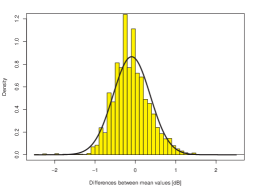
(a) Distribution of errors for the LOS experiment

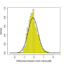
(b) Distribution of errors for the non-LOS experiment

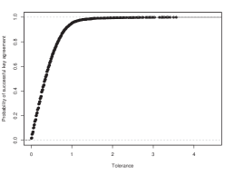
(c) Success probability of key generation based on all positions.

Figure 4: Deviations in the channel and the resulting success rate of key generations in our experiments.

5.1 WSN Testbed and Methodology

The experiments were conducted over several days on a university floor, that is, an indoor setting across several rooms. During the measurements, several wireless LAN access points were concurrently operating in the 2.4 GHz band; so, the experiments were performed in a real-world environment with unpredictable factors. The environment contains concrete walls, as well as office furniture made of different materials. Especially metal objects such as shelves and cabinets with good reflection properties regarding electromagnetic waves were present. Thus, this set of environment can be considered to generate a rich multipath effects, while it also represents a typical indoor scenario. An additional factor for this changing environment was the movement of people in corridors or office rooms.

Several different scenarios were considered to evaluate the impact of positioning on secrecy and robustness. A large meeting room was used for experiments, where the sensor motes always maintained a line of sight connection, and several smaller office rooms were used to quantify the impact of shadowing objects and walls. For each of these scenarios, 250 positions were considered, and the distance was kept constantly at 2.5 meters to avoid the influence of path loss effects. In long-term and dynamic scenarios, these rooms and the connecting corridors were used, and 1000 additional positions were tested with mixed distances and obstacles. We used $k=16$ samples on each channel, collected on $n=16$ channels.

5.2 Protocol Robustness

In order to evaluate the robustness of the protocol, a total of 1600 positions of the two parties was tested, and the measurements and deviations between the two parties recorded for each of the 16 channels.

From the deviations $N=N_{\mathrm{Alice}}-N_{\mathrm{Bob}}$ observed, we can see that they are bounded. The histogram of deviations is given in Fig. 4a and 4b, which also shows that these deviations are fitted well by a zero-mean Normal distribution with a standard deviation of $\sigma=0.461$ dB in the LOS experiment and $\sigma=0.503$ dB in the non-LOS experiment. The empirical distributions have even lighter tails than the fitted Normal distributions. We can use this knowledge to evaluate the success probability as described in Section 4.3 for protocol optimizations. Based on the experiments, we can conclude that the reciprocity of the wireless channel is very strong.

The success ratio of the protocol can be directly controlled by the tolerance values of the code used, as codes with larger tolerance values are able to correct stronger deviations. With a tolerance of 1 dB, 94.6 % of the key agreements are successful on the first run. This value is increased to 99.2 % with a tolerance of 2 dB. The empirical cumulative distribution function (ECDF) of all experiments is shown in Fig. 4c. The majority of deviations are below 2 dB, and only a small number of extreme outliers were measured. As the chosen tolerance value also has an impact on the secrecy of the resulting bit string, a careful trade-off between secrecy and robustness must be found.

5.3 Evaluation of the Channel Entropy

We evaluated the frequency-selective channel fading effects in two different environmental settings: (i) connections with line of sight only; and (ii) connections with obstacles in the direct connection, that is, non-LOS connections. The LOS experiment was intended as the worst-case scenario because a strong LOS component may be able to dominate the multipath fading behavior. Yet, our experiments show that this is not the case, and both experiments yield roughly the same entropy. In all experiments, several different tolerance values were considered to show the impact of this parameter on the secrecy.

UACEGIOQMCACOIMOOOOMMOWMIMMIOQOOOQSSQMIIKMMOACCAACIMCAAOSU MMMOOQaOKKMMMIMOMGGOKCECCGKAAAACAAACCECCESQOMMSUMKIKQQSOMQ QMKKOQQOUSOOQQSCGECAAAGEEIOKKQaSMIIGGIOaOKMUQKQOMOMMOMKSQM MMIMQOMOMMOMKSQMMMIMWQOMQQWOUQOQOOEEIaMOIGKIMSICEGMMECEKSO IMMGIIGIOOIIIKOUOQQQWQSaUa9ACAKIIKMOMMOGGEAACKEEAAACAEOIEC KQMOQUSOOOUUUSMIACCAACIMCAAMIGIIECEIMOOSMGGMEEGIMMIIOMGEGO MSaKEEEECCCEMOMOOEEAAACAEOIECMMIIGEGKIKQSKIKKEAAOIEACECAKG AACESMECCEECCCCAEGEACEICACIIIIQSOMMIIOQOaQGCAAAEIIEEIOMMaS MOOMIKECEKGCEMKEAOOOUaQSOMMQUSQMOCGKSECAACGQOIKEEIEGECGGGG GOMIEMKCCECAMEEIEGECGGGIIMKIMIEECGMSMMMOIGGGOOOGGIKKOOMOOO 955;;IQMCCEIMIMOSQIOI???CGKOSKIIGECEIKMMOQMMIECEGECCESUaWU WWWWUaWSSSS??A????CIQMMMMIEOSSOOMOIIMKMMIIOCCAACEIECEEIMGE QOOOUSOMKMMQKECGOMIIKMS[WQQOGE??ACGGEAAAAA??==AA?ACEEAACCC ECOOOGKGEEGGGKMOUUKGGKGIMMIKOMMOMMQQOOQOOOUSOMKMMQGGKGEIMM

Figure 5: A part of the T-string used for estimating the Shannon entropy of codewords generated by our key-generation protocol. This approach is based on encoding the codewords as ASCII strings and analyzing their minimal representation.

The secrecy analysis focuses on the distribution of signal strength measurements, especially on the entropy that these distributions offer. The evaluation of the entropy for single channels is straightforward: we use the empirical distribution to calculate $\mathrm{H}\left(C_{i}\right)$ for each of the $n$ channels individually, using the relative frequencies as the estimates of codeword probabilities. For example, this analysis shows that there are 3.5 secret bits available from each channel for a tolerance value of $t=1$; a value of $t=0.5$ results in an increase to 4.38 bit.

The joint entropy under the assumption of independent channels is the sum of the channels’ entropy values. However, the independence cannot be assumed as the channels are within the coherence bandwidth, and using the conventional approach to estimate the Shannon entropy of dependent channels using sampling is not effective, as this becomes prohibitive in spaces with larger dimensions. For example, to show a joint secrecy of 45 bit, at least $2^{45}$ samples must be collected. Additionally, the unknown dependency structure of the generated secret strings makes such quantification harder. The reason is that the Shannon entropy operates on the knowledge of the underlying joint distribution, which is unknown in our case. While in the next section we derive a stochastic model for such analysis, we are still interested in finding out how much uncertainty is present in the experimental data without any assumptions on the underlying codeword distribution, i.e., without requiring any a priori knowledge. The idea we follow is based on construction complexity described by the notion of T-complexity [25]. T-complexity quantifies the difficulty to decompose input strings into codewords of T-codes, i.e., the complexity when trying to find the minimal representation of the input string. Speidel et al. [23] show in their work that T-complexity is the fastest to converge to the true value of the Shannon entropy, and provide an algorithm that enables fast computations of entropy values. The tool tcalc [32], developed by the same group, was used to evaluate our results. As this tool operates on byte strings, we had to convert the lists of quantized values to arrays consisting of different ASCII characters as input. These characters were concatenated to form a large string that can be used as input to tcalc. A part of the T-string used is given in Fig. 5.

As a result, using this method we were able to capture the dependencies between channels in the empirical data without explicitly knowing them. The results from this analysis are discussed in the next subsection and in Section 6.1 we use them for the validation of the derived stochastic model.

Figure 6: Results for the implementation on MICAz sensor motes. The amount of secrecy under different dependency assumptions is shown, with the corresponding success probabilities of key agreement.

5.3.1 Results from Experimental Analysis

A comparison of results showing the available entropy from the experimental data is shown in Fig. 6. With a tolerance value of $t=1$, the entropy under independence assumption is 56 bit for both LOS and non-LOS connections. When considering the dependencies in the measurements, 31 bit of entropy can be achieved with the limited number of channels and precision that the wireless sensor mote hardware offers. Lower tolerance values can be used to increase secrecy. For example, a tolerance value of 0.4, which results in a 56 % chance of successful key agreement, offers 45–50 secret bits under dependent channels.

The entropy of generated shared secrets in this settings can be compared with conventional password-based security schemes and applied to the protocols such as, for example, commitment-based authentication protocols using short authenticated (e.g., [26, 19, 13, 10]). Similarly, protocols such as the Encrypted Key-Exchange (EKE) apply short shared secrets for confidential exchange of public key material (e.g., [3, 24]). The shared secrets in such applications are usually created by the user and contain approximately 18 bit entropy due to dependency between characters (for a comprehensive overview of password entropy, see [21]). Since these protocols protocols play an important role in wireless networks as a part of device-pairing schemes, generating secrets from the wireless channel can be seen as their valuable extension and alternative to an user-required input of secrets.

6 Increasing the Length of a Secret

The experimental analysis shows that the dependencies between channels have considerable influence on the secrecy of the proposed protocol. In contrast to previous section, we now develop a stochastic model that makes these dependencies explicit and enables us to analyze and predict ways to increase the achievable secrecy. Especially, we want to answer questions such as: what is the impact of increasing the number of available channels, and increasing the spacing between center frequencies. To derive a realistic model of dependent wireless channels, we start with fitting and validating the distribution of single channel measurements and then extending it to a multivariate case, which captures the dependencies between wireless channels. The model is validated by comparing the resulting entropy values with our empirical results.

6.1 Modeling Channel Dependency

Frequently used distributions for large-scale models of wireless channels are Rayleigh, Ricean, or Log-Normal [20] depending on the properties of the respective propagation environment. Also, in scenarios common to WLANs and WSNs, where distances between transceivers are short, the empirical data can be approximated by the Normal distribution [22, 12, 5]. To find an adequate distribution, we collected 4000 RSS sample means for each of the LOS and non-LOS scenarios, where every RSS mean was calculated over 16 measurements, estimating the distribution parameters using Maximum Likelihood Estimation (MLE). The resulting fit of the Rayleigh and Normal distributions to the empirical data is shown in Fig. 7a. Additionally, we tested the normality of the sampled data using the probability plot correlation coefficient test for normality (PPCC), which is based on checking for linearity between the theoretical quantiles and the sample data [8]. In fact, the goodness of fit test confirms that the Normal distribution (correlation coefficient $=0.992$) can be assumed with an even higher confidence than the corresponding Rayleigh distribution (correlation coefficient $=0.967$). In this case, the multivariate Normal distribution can be used to describe the complex dependency structures of wireless channels by directly estimating the covariance matrix from the empirical data.

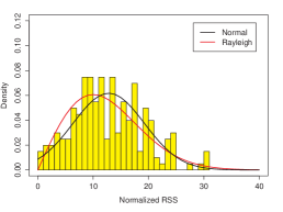
(a) Fitting of different distributions to the empirical data.

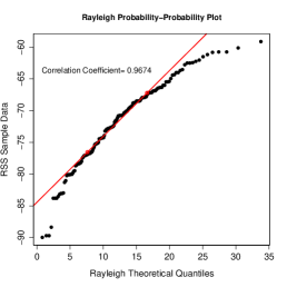
(b) Rayleigh Probability-Probability test

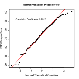
(c) Normal Probability-Probability test

Figure 7: Test for different distributions of the empirical data.

Hence, to analyze the dependencies of the joint distribution over all 16 wireless channels, especially with respect to the joint entropy, we model the signal strength values of different channels using a single 16-dimensional multivariate Normal distribution. The distribution parameter estimation is straightforward: the vector of mean values $\mu$, which is in case of the Normal distribution already the MLE for the population mean, and for the covariance matrix $\varSigma$ we used the MLE method:

$$\hat{\varSigma}=\frac{1}{k-1}\sum_{j=1}^{k}\left(\boldsymbol{m}^{(j)}-\boldsymbol{\mu}\right)\left(\boldsymbol{m}^{(j)}-\boldsymbol{\mu}\right)^{T}.$$

Finally, we validated the multivariate channel dependency model against our empirical data by using the same error correction mechanism (described in Section 4) to generate secret strings and to compare the Shannon entropy of the empirical data with the results of the model. The results of this evaluation are given in Fig. 8, which shows the resulting entropy values for the non-LOS data applying the same analysis methods used in the experimental analysis. The LOS experiment is omitted as the behavior is similar. The model captures the dependency structure well, resulting in a similar progression of the curve for the existing tolerance values, although the entropy is slightly overestimated by the model.

Figure 8: Comparison of discrete entropy values based on RSS values generated using the stochastic model.

Using this model, we can estimate the amount of entropy if additional resources are available, such as a higher number of channels or a larger spacing between channels. We only need to consider the properties of the covariance matrix $\varSigma$ with respect to entropy. The differential entropy (in natural units) of the multivariate Normal distribution is given by

$$H_{\mathrm{mv}\mathcal{N}}=\frac{1}{2}\ln\left(\left(2\pi\mathrm{e}\right)^{n}\det\varSigma\right),$$ (1)

depending on the number of channels $n$ and the determinant of $\varSigma$. The first-order effect of increasing the number of channels is easy to quantify, the differential entropy is increased by $2.05$ bit for each additional channel. However, the relationship is not obvious with respect to the determinant. In the case of independence, only the main diagonal of the covariance matrix is populated, but in the general case the complete matrix has an influence that is hard to quantify.

6.2 More Channels or Larger Frequency Spacing

First, we consider the effects of the determinant on the security given a larger number of channels. To this end, we extrapolate the covariance matrix and evaluate the effect on the determinant.

Two different prediction methods are used, one that extrapolates $\varSigma$ directly and another that also simulates the effect of larger spacing between center frequencies and then extrapolates the matrix.

We used $\left(i{\times}i\right)$ sub-matrices with $i=1,\ldots,15$ of the matrix $\varSigma$ to predict the $16{\times}16$ matrix $\varSigma$. Only the values contained in the sub-matrix are used, in the following manner: each diagonal is treated independently, as it represents a different lag in the covariances. The missing elements of the matrix are chosen uniformly from a range between minimum and maximum values on the respective diagonal. The results of this $16{\times}16$ prediction for the non-LOS experiment are shown in Fig. 9. A sample of 100 extrapolated covariance matrices was used to predict the known amount of differential entropy for 16 channels, the used confidence level in the graph is 95 %. The horizontal line represents a differential entropy using the correct $\varSigma$ from the experiments. The predicted entropy values using different sub-matrix sizes are shown, obtained from mean values of different uniform extrapolations. Even with small $2{\times}2$ prediction matrices, it is possible to estimate the entropy accurately. The evaluation for the LOS experiment is not shown, but gave similar results. Thus, we can use the estimation of $\varSigma$ to predict the secrecy from a larger number of channels.

The second matrix extrapolation method was used to evaluate the effects of a larger spacing between the channels. Only every second (third, $n$-th) diagonal was used and the remaining ones were removed for this analysis. This simulates a channel spacing of 10 MHz (15 MHz, $5n$ MHz). This smaller matrix is then extrapolated in the same fashion as described before. The quality of prediction is comparable to the previous results.

Figure 9: Prediction of the differential entropy using only a subset of available channels. Even with a small number of channels, an accurate prediction is possible.

Fig. 10 shows the increases of entropy we can observe from our model. The figure shows the results of the non-LOS experiment only, but the LOS experiment gave similar results. The results are given in differential entropy, which does not take the tolerances into account. The lowest line describes the increase in joint differential entropy if we use the same determinant we obtained from 16 channels. This results in an increase of 2.05 bit for each channel, but it is also a very conservative prediction, it overestimates the dependencies between channels with center frequencies far apart from each other. Using extrapolation based on the $16{\times}16$ matrix and calculating the entropy using Eq. (1) and the new $\varSigma$, we see an increase of 4.02 bit for each additional channel. The slashed line shows an additional gain if the channels are spaced 10 MHz apart, instead of the 5 MHz spacing in our experiments, yielding a 4.25 bit increase. Our model shows that there are several ways to increase the secrecy of the proposed protocol. With measurements of higher precision it is possible to generate more bits on each channel, but as this increases the hardware costs, it is advisable to rather use a larger number of channels.

\psfrag{Number of channels}{\small{Number of channels}}\psfrag{Joint differential entropy}{\small{Joint differential entropy (bit)}}\psfrag{Fixed determinant}{\footnotesize{\!Fixed $\det\left(\varSigma\right)$}}\psfrag{Extrapolated determinant}{\footnotesize{Extrapolated $\det\left(\varSigma\right)$}}\psfrag{10MHz spacing}{\footnotesize{~{}~{}~{}~{}~{}10\,MHz spacing}}\psfrag{0}[1][0]{\scriptsize{$0$}}\psfrag{10}[1][0]{\scriptsize{$10$}}\psfrag{20}[1][0]{\scriptsize{$20$}}\psfrag{30}[1][0]{\scriptsize{$30$}}\psfrag{40}[1][0]{\scriptsize{$40$}}\psfrag{50}[1][0]{\scriptsize{$50$}}\psfrag{60}[1][0]{\scriptsize{$60$}}\psfrag{70}[1][0]{\scriptsize{$70$}}\psfrag{80}[1][0]{\scriptsize{$80$}}\psfrag{90}[1][0]{\scriptsize{$90$}}\psfrag{100}[1][0]{\scriptsize{$100$}}\psfrag{110}[1][0]{\scriptsize{$110$}}\psfrag{120}[1][0]{\scriptsize{$120$}}\psfrag{130}[1][0]{\scriptsize{$130$}}\psfrag{140}[1][0]{\scriptsize{$140$}}\psfrag{50}[1][0]{\scriptsize{$50$}}\psfrag{100}[1][0]{\scriptsize{$100$}}\psfrag{150}[1][0]{\scriptsize{$150$}}\psfrag{200}[1][0]{\scriptsize{$200$}}\psfrag{250}[1][0]{\scriptsize{$250$}}\psfrag{300}[1][0]{\scriptsize{$300$}}\psfrag{-5.5}[1][0]{\scriptsize{-$5.5$}}\psfrag{-5}[1][0]{\scriptsize{-$5$}}\psfrag{-4.5}[1][0]{\scriptsize{-$4.5$}}\psfrag{-4}[1][0]{\scriptsize{-$4$}}\psfrag{-3.5}[1][0]{\scriptsize{-$3.5$}}\psfrag{-3}[1][0]{\scriptsize{-$3$}}\psfrag{-2.5}[1][0]{\scriptsize{-$2.5$}}\psfrag{-2}[1][0]{\scriptsize{-$2$}}\psfrag{-1.5}[1][0]{\scriptsize{-$1.5$}}\psfrag{-1}[1][0]{\scriptsize{-$1$}}\psfrag{-0.5}[1][0]{\scriptsize{-$0.5$}}\psfrag{0}[1][0]{\scriptsize{$0$}}\psfrag{0.5}[1][0]{\scriptsize{$0.5$}}\psfrag{1}[1][0]{\scriptsize{$1$}}\psfrag{1.5}[1][0]{\scriptsize{$1.5$}}\psfrag{2}[1][0]{\scriptsize{$2$}}\psfrag{2.5}[1][0]{\scriptsize{$2.5$}}\psfrag{3}[1][0]{\scriptsize{$3$}}\psfrag{3.5}[1][0]{\scriptsize{$3.5$}}\psfrag{4}[1][0]{\scriptsize{$4$}}\psfrag{4.5}[1][0]{\scriptsize{$4.5$}}\psfrag{5}[1][0]{\scriptsize{$5$}}\psfrag{5.5}[1][0]{\scriptsize{$5.5$}}\psfrag{6}[1][0]{\scriptsize{$6$}}\psfrag{8}[1][0]{\scriptsize{$8$}}\psfrag{10}[1][0]{\scriptsize{$10$}}\psfrag{12}[1][0]{\scriptsize{$12$}}\psfrag{14}[1][0]{\scriptsize{$14$}}\psfrag{16}[1][0]{\scriptsize{$16$}}\psfrag{18}[1][0]{\scriptsize{$18$}}\includegraphics[width=216.81pt]{figures/extrapolate-Sigma/eps/plus/space/extrapolate-Sigma-plus-unif-los}

Figure 10: Extrapolation of covariance matrix $\varSigma$ for a larger number of channels to evaluate of the model with respect to secrecy gains.

7 Conclusion

Secret key generation and distribution poses one of the main security challenges in wireless networks, especially in computation-limited WSNs. In conventional security schemes, the wireless channel is usually considered as a part of an adversarial toolbox which additionally helps to launch different attacks by abusing its broadcast nature. Yet, in recent years a number of papers following an alternative approach to wireless security have demonstrated that the unpredictable and erratic nature of wireless communication can be used to enhance and augment conventional security designs. Taking advantage of physical properties of signal propagation, mutual secrets between wireless transmitters can be derived. While this approach for securing wireless networks has been recently addressed in [15, 2], both contributions require movement as the main generator of secret material. Although valuable to mobile networks, such solutions are not applicable to the majority of WSN applications which are based on static sensor motes.

The main focus of this work was to overcome this limitation. We started by introducing a system model based on real-world measurements using IEEE 802.15.4 technology, and describing building blocks of a novel key generation protocol. To demonstrate its applicability, the protocol was implemented and evaluated using MICAz sensor motes. Experiments show that the protocol is able to successfully generate keys in over 95 % of the cases, irrespective of environmental properties. By using only a very limited number of wireless channels, the proposed protocol can already provide secrets up to 50 bit, depending on the wireless channel behavior. A stochastic model derived in this work validated our experimental data and provided guidelines on how to increase the length of the secret keys based on either increasing the number of wireless channels or increasing the channel spacing. For example, if the number of channels of the present IEEE 802.15.4 is set to 40, this protocol can generate up to 160 bit secret keys in static scenarios.

The possibility to increase the length of a secret by using additional wireless channels or larger frequency spacing is an interesting alternative to computational-based approaches not only from the security perspective but also from the network throughput perspective. For example, cognitive radio is focused on increasing the utilization of limited radio resources by dynamically adjusting the transmission to interference-free frequencies. The key generation protocol introduced in this work can inherently take advantage of such technologies.

Finally, this approach to key generation is intended to extend and support conventional security designs as it only needs a limited number of messages exchanges to generate shared secrets even on the currently available, off-the-shelf WSN devices.

References

- [1] Tomoyuki Aono, Keisuke Higuchi, Makoto Taromaru, Takashi Ohira, and Hideichi Sasaoka. Experiments of IEEE 802.15.4 ESPARSKey (Encryption Scheme Parasite Array Radiator Secret Key) - RSSI Interleaving Scheme. In IEICE Tech. Rep., volume 105, pages 31–36, Kyoto, April 2005.
- [2] Babak Azimi-Sadjadi, Aggelos Kiayias, Alejandra Mercado, and Bülent Yener. Robust Key Generation from Signal Envelopes in Wireless Networks. In CCS ’07: Proceedings of the 14th ACM Conference on Computer and Communications Security, pages 401–410, New York, NY, USA, 2007. ACM.
- [3] Steven M. Bellovin and Michael Merritt. Encrypted key exchange: Password-based protocols secure against dictionary attacks. In Proceedings of the 1992 IEEE Symposium on Security and Privacy, pages 72–85, May 1992.
- [4] Charles Bennett and Gilles Brassard. Quantum cryptography: Public key distribution and coin tossing. In Proceedings of IEEE International Conference on Computers, Systems, and Signal Processing, pages 175–179, 1984.
- [5] Atreyi Bose and Chuan Heng Foh. A Practical Path Loss Model For Indoor WiFi Positioning Enhancement. In The 6th International Conference on Information, Communications & Signal Processing, pages 1–5, December 2007.
- [6] Seyit A. Çamtepe and Bülent Yener. Key Distribution Mechanisms for Wireless Sensor Networks: a Survey, March 2005. Technical Report TR-05-07 Renesselaer Polytechnic Institute, Computer Science Department.
- [7] Artur K. Ekert. Quantum cryptography based on Bell’s theorem. Physical Review Letters, 67(6):661+, 1991.
- [8] James J. Filliben. The Probability Plot Correlation Coefficient Test for Normality. Technometrics, 17(1):111–117, February 1975.
- [9] Steven J. Fortune, David M. Gay, Brian W. Kernighan, Orlando Landron, Reinaldo A. Valenzuela, and Margaret H. Wright. WISE Design of Indoor Wireless Systems: Practical Computation and Optimization. IEEE Computational Science & Engineering, 2(1):58–68, 1995.
- [10] Oded Goldreich and Yehuda Lindell. Session-Key Generation Using Human Passwords Only. Technical report, Jerusalem, Israel, Israel, 2000. Technical Report: MCS00-15.
- [11] Suman Jana, Sriram Nandha Premnath, Mike Clark, Sneha K. Kasera, Neal Patwari, and Srikanth V. Krishnamurthy. On the effectiveness of secret key extraction from wireless signal strength in real environments. In MobiCom ’09: Proceedings of the 15th annual international conference on Mobile computing and networking, pages 321–332, New York, NY, USA, 2009. ACM.
- [12] Kamol Kaemarungsi and Prashant Krishnamurthy. Modeling of Indoor Positioning Systems Based on Location Fingerprinting. In Proceedings of the 23rd Annual Joint Conference of the IEEE Computer and Communications Societies (INFOCOM), volume 2, pages 1012–1022, March 2004.
- [13] Jonathan Katz, Rafail Ostrovsky, and Moti Yung. Efficient and Secure Authenticated Key Exchange Using Weak Passwords. Journal of the ACM (JACM), 57(1):1–39, 2009.
- [14] An Liu and Peng Ning. TinyECC: A Configurable Library for Elliptic Curve Cryptography in Wireless Sensor Networks. In IPSN’08: Proceedings of the International Conference on Information Processing in Sensor Networks, pages 245–256, 2008.
- [15] Suhas Mathur, Wade Trappe, Narayan Mandayam, Chunxuan Ye, and Alex Reznik. Radio-telepathy: Extracting a Secret Key from an Unauthenticated Wireless Channel. In MobiCom ’08: Proceedings of the 14th ACM International Conference on Mobile Computing and Networking, pages 128–139, New York, NY, USA, 2008. ACM.
- [16] Ueli Maurer. Protocols for Secret Key Agreement by Public Discussion Based on Common Information. In Advances in Cryptology — CRYPTO ’92, volume 740 of Lecture Notes in Computer Science, pages 461–470. Springer-Verlag, August 1993.
- [17] Ueli Maurer, Renato Renner, and Stefan Wolf. Unbreakable keys from random noise. In P. Tuyls, B. Skoric, and T. Kevenaar, editors, Security with Noisy Data, pages 21–44. Springer-Verlag, 2007.
- [18] Ueli Maurer and Stefan Wolf. Secret-Key Agreement Over Unauthenticated Public Channels - Parts I-III. IEEE Transactions on Information Theory, 49(4):822–851, April 2003.
- [19] Minh-Huyen Nguyen and Salil Vadhan. Simpler Session-Key Generation from Short Random Passwords. Journal of Cryptology, 21(1):52–96, 2008.
- [20] Theodore Rappaport. Wireless Communications: Principles and Practice. Prentice Hall PTR, 2001.
- [21] Thomas Schürmann and Peter Grassberger. Entropy estimation of symbol sequences. CHAOS, 6:414, 1996.
- [22] Yong Sheng, Keren Tan, Guanling Chen, David Kotz, and Andrew Campbell. Detecting 802.11 MAC layer spoofing using received signal strength. In Proceedings of the 27th Annual Joint Conference of the IEEE Computer and Communications Societies (INFOCOM), pages 1768–1776, April 2008.
- [23] Ulrich Speidel, Mark Titchener, and Jia Yang. How well do practical information measures estimate the Shannon entropy? In CSNDSP ’06: Proceedings of the 5th International Symposium on Communication Systems, Networks and Digital Signal Processing, pages 861–865. IEEE, 2006.
- [24] Michael Steiner, Gene Tsudik, and Michael Waidner. Refinement and Extension of Encrypted Key Exchange. SIGOPS Oper. Syst. Rev., 29:22–30, July 1995.
- [25] Mark R. Titchener, Radu Nicolescu, Ludwig Staiger, T. Aaron Gulliver, and Ulrich Speidel. Deterministic Complexity and Entropy. Fundamenta Informaticae, 64(1-4):443–461, 2005.
- [26] Serge Vaudenay. Secure Communications over Insecure Channels Based on Short Authenticated Strings. In Advances in Cryptology - CRYPTO 2005: 25th Annual International Cryptology Conference, pages 309–326, 2005.
- [27] Arvinderpal Wander, Nils Gura, Hans Eberle, Vipul Gupta, and Sheueling Chang Shantz. Energy Analysis of Public-Key Cryptography for Wireless Sensor Networks. In PerCom ’05: Proceedings of the third annual IEEE International Conference on Pervasive Computing and Communications, pages 324–328, March 2005.
- [28] Matthias Wilhelm, Ivan Martinovic, and Jens B. Schmitt. On Key Agreement in Wireless Sensor Networks based on Radio Transmission Properties. In Proceedings of the 5th Annual Workshop on Secure Network Protocols (NPSec) in conjunction with IEEE ICNP 2009, pages 37–42, Princeton, New Jersey, USA, October 2009. IEEE Computer Society.
- [29] Matthias Wilhelm, Ivan Martinovic, and Jens B. Schmitt. Secret Keys from Entangled Sensor Motes: Implementation and Analysis. In Proceedings of the 3rd ACM Conference on Wireless Network Security (WiSec 2010), Hoboken, NJ, USA., March 2010. ACM Press.
- [30] Robert Wilson, David Tse, and Robert A. Scholtz. Channel Identification: Secret Sharing using Reciprocity in Ultrawideband Channels. In ICUWB ’07: IEEE International Conference on Ultra-Wideband, pages 270–275, sep 2007.
- [31] Yang Xiao, Venkata Krishna Rayi, Bo Sun, Xiaojiang Du, Fei Hu, and Michael Galloway. A Survey of Key Management Schemes in Wireless Sensor Networks. Computer communications, 30(11-12):2314–2341, 2007.
- [32] Jia Yang and Ulrich Speidel. A Fast T-decomposition Algorithm. Journal of the UCS, 11(6):1083–1101, 2005.
- [33] Kai Zeng, Daniel Wu, An Chan, and Prasant Mahapatra. Exploiting Multiple-Antenna Diversity for Shared Secret Key Generation in Wireless Networks. In Proceedings of the 29th IEEE Conference on Computer Communications (INFOCOM), San Diego, CA, March 2010.