On leave of absence from the ] Center for Nuclear Physics, Institute of Physics, Hanoi, Vietnam

Canonical and microcanonical ensemble descriptions
of thermal pairing within BCS and quasiparticle RPA

Abstract

We propose a description of pairing properties in finite systems within the canonical and microcanonical ensembles. The approach is derived by solving the BCS and self-consistent quasiparticle random-phase approximation with the Lipkin-Nogami particle-number projection at zero temperature. The obtained eigenvalues are embedded into the canonical and microcanonical ensembles. The results obtained are found in quite good agreement with the exact solutions of the doubly-folded equidistant multilevel pairing model as well as the experimental data for ⁵⁶Fe nucleus. The merit of the present approach resides in its simplicity and its application to a wider range of particle number, where the exact solution is impracticable.

The study of thermodynamic properties of finite systems such as atomic nuclei or ultra-small metallic grains has been an important topic in nuclear physics. Thermodynamic properties are usually described within the grand canonical ensemble (GCE), canonical ensemble (CE), or microcanonical ensemble (MCE). The GCE consists of identical systems in thermal equilibrium, each of which exchanges its energy and particle number with the external reservoir. The systems of the CE exchange only their energies whereas the particle number is fixed. The MCE consists of thermally isolated systems with the same energy and particle number. Among these ensembles, the GCE is often used in the theoretical studies because of convenience in the calculations of thermodynamic quantities. For example, the well-known BCS theory of superconductivity BCS was derived based on the GCE. This theory describes very well thermodynamic properties of infinite systems such as metal superconductors, where quantal and thermal fluctuations are zero. The latter, however, have been shown to be quite significant in finite small systems Moretto ; SPA ; Zele ; MBCS ; FTBCS1 ; Ensemble . They smoothed out the superfluid-normal (SN) phase transition, which is a typical property of infinite systems. Most of theoretical approaches to thermal pairing have been derived so far within the GCE in finite systems such as atomic nuclei, where no particle-number fluctuations are allowed. Therefore, the CE and MCE should be used instead. Moreover, the exact eigenvalues of the pairing problem Exact are usually embedded into the CE and MCE Ensemble ; Sumaryada . But this task is impracticable for particle numbers $N>$ 14 in the case of half-filled doubly-folded multilevel model with $N=\Omega$ ($\Omega$ is number of single-particle levels). The reason is that the exact partition function at finite temperature $T\neq$ 0 should include all excited states. The finite-temperature shell-model Monte Carlo (FTSMMC) SMMC1 ; SMMC2 has also been used to evaluate the partition function, but it is very time consuming and cannot be applied to heavy nuclei. The FTSMMC cannot be applied to the MCE either because it is impossible to include all the microstates of the system. It is therefore highly desirable to construct an approach based on the CE and MCE, which can offer results in good agreement with the exact solutions for any value of the particle number, as well as with experimental data for realistic nuclei. This is the goal of the present study.

We consider the pairing Hamiltonian $H=\sum_{j}\epsilon_{j}\hat{N}_{j}-G\sum_{jj^{\prime}}\hat{P}_{j}^{\dagger}\hat{P}_{j^{\prime}}~{}$, where $\hat{N}_{j}=\sum_{m}a_{jm}^{\dagger}a_{jm}$ is the particle-number operator, and $\hat{P}_{j}=\sum_{m>0}a_{jm}^{\dagger}a_{j\tilde{m}}^{\dagger},\hat{P}_{j}=(\hat{P}_{j}^{\dagger})^{\dagger}$ are the pairing operators. The operators $a_{jm}^{\dagger}$ and $a_{jm}$ are respectively the creation and destruction operators of a nucleon moving on the $j$-th orbital ($a_{j\tilde{m}}=(-)^{j-m}a_{j-m}$). This Hamiltonian has been diagonalized exactly in Exact to obtain n_Exact=$\sum_{S}{\rm C}_{S}^{\Omega}\times{\rm C}_{N_{\rm pair}-S/2}^{\Omega-S}$ eigenstates with eigenvalues $\varepsilon_{S}^{\rm Exact}$ and occupation numbers $f_{j}^{S}$, where S = 0, 2, … $\Omega$ is the total seniority of the system and C${}_{m}^{n}=m!/[n!(m-n)!]$ Ensemble . The exact partition function is constructed by embedding the exact eigenvalues into the CE as $Z_{\rm Exact}(\beta)=\sum_{S}d_{S}\exp({-\beta\varepsilon_{S}^{\rm Exact}})$ , with the degeneracy $d_{S}=2^{S}$ and inverse temperature $\beta=1/T$. Knowing the partition function $Z$, one calculates the free energy $F$, entropy $S$, total energy ${\cal E}$, heat capacity $C$, and pairing gap $\Delta$ as $F=-T{\rm ln}Z(T)$, $S=-{\partial F}/{\partial T}$, ${\cal E}=F+TS$, $C={\partial{\cal E}}/{\partial T}$, and $\Delta=[-G({\cal E}-2\sum_{j}\epsilon_{j}f_{j}+G\sum_{j}f_{j}^{2})]^{1/2}$, where $f_{j}$ are the occupation numbers on the $j$th orbital obtained by averaging the state-dependent occupation numbers $f_{j}^{(S)}$ within the CE Ensemble . The conventional BCS theory at $T\neq$ 0 (FTBCS) is derived by using the variational procedure with respect to the quasiparticle Hamiltonian ${\cal H}$. The latter is obtained by applying the Bogoliubov’s transformation of the pairing Hamiltonian $H$ from the particle operators, $a_{jm}^{\dagger}$ and $a_{jm}$, to the quasiparticle ones, $\alpha_{jm}^{\dagger}$ and $\alpha_{jm}$. The variational procedure is carried out on the average quantities within the GCE, namely $\langle{\cal\hat{O}}\rangle\equiv{\rm Tr}[{\cal\hat{O}}e^{-\beta({\cal H}-\lambda\hat{N})}]/{\rm Tr}[e^{-\beta({\cal H}-\lambda\hat{N})}]$ for any observable $\hat{O}$ with $\lambda$ being the chemical potential determined as the Lagrangian multiplier to preserve the average particle number $\langle\hat{N}\rangle=N$. Therefore the conventional FTBCS theory is called the GCE-BCS in the present article.

The CE description of thermal pairing can be undertaken in two directions. The first one is to apply the exact particle-number projection (PNP) at finite temperature on top of the GCE theory Nakada ; PNP . This approach is rather complicated for realistic nuclei. The second direction, which the present study follows, is to embed the solutions of a theoretical approximation at zero temperature, which conserves the particle number, into the CE. We employ the solutions of the BCS equations with PNP within the Lipkin-Nogami method LN (LNBCS) for each total seniority $S$ and embed the eigenvalues $\varepsilon_{S}^{\rm LNBCS}$ obtained at $T$=0 into the CE. The partition function of the so-called CE-LNBCS approach is then given as

$$Z_{\rm LNBCS}(\beta)=\sum_{S}d_{S}e^{-\beta\varepsilon_{S}^{\rm LNBCS}}~{}.$$ (1)

Using it, we can obtain the free energy, entropy, total energy and heat capacity as has been discussed above, by replacing $Z_{\rm Exact}(\beta)$ with $Z_{\rm LNBCS}(\beta)$. As for the pairing gap, it is obtained by averaging the gaps $\Delta_{S}^{\rm LNBCS}$, which are the solutions of the LNBCS equations at $T=0$, namely

$$\Delta={Z_{\rm LNBCS}(\beta)^{-1}}\sum_{S}\Delta_{S}^{\rm LNBCS}d_{S}e^{-\beta\varepsilon_{S}^{\rm LNBCS}}~{}.$$ (2)

Within the BCS theory at $T=0$, only the lowest eigenstates can be obtained, e.g the ground-state energy for $S$=0. The total number of the LNBCS eigenstates embedded into the CE is equal to n${}_{\rm LNBCS}=\sum_{S}{\rm C}_{S}^{\Omega}$, which is much smaller than n_Exact. The CE of these lowest eigenstates is therefore comparable with the exact one only in the region of low $T$. At higher $T$, one needs to include not only the ground state but also excited states into the CE. This can be resolved by means of the selfconsistent quasiparticle RPA with Lipkin-Nogami PNP (LNSCQRPA) SCQRPA . The LNSCQRPA includes the ground-state and screening correlations, which are neglected within the conventional BCS and QRPA. The importance of these correlations in finite systems has been demonstrated in SCQRPA . They improve the agreement between the energies of ground state and low-lying excited states obtained within the LNSCQRPA and the corresponding exact results for the doubly-folded multilevel pairing model. The formalism of the LNSCQRPA was presented in details in SCQRPA , so we do not repeat it here. The total number of eigenstates obtained within the LNSCQRPA is n${}_{\rm LNSCQRPA}=\sum_{S}{\rm C}_{S}^{\Omega}\times(\Omega-S)>$n_BCS because of the presence of QRPA excited states , but it is still much smaller than n_Exact. For example, for the half-filled model with $\Omega=N=10$, n${}_{\rm Exact}=8953$, whereas n${}_{\rm LNBCS}=512$ and n${}_{\rm LNSCQRPA}=2561$. The thermodynamic quantities are obtained within the CE-LNSCQRPA in the same way as that for the CE-LNBCS (1), namely from the CE-LNSCQRPA partition function $Z_{\rm LNSCQRPA}(\beta)=\sum_{S}d_{S}\exp[-\beta\varepsilon_{S}^{\rm LNSCQRPA}]$, where $\varepsilon_{S}^{\rm LNSCQRPA}$ are the eigenvalues obtained by solving the LNSCQRPA equations for each total seniority $S$.

Within the MCE description, we use the eigenvalues $\varepsilon_{S}^{\rm LNBCS}$ and $\varepsilon_{S}^{\rm LNSCQRPA}$ to calculate the MCE entropy directly from the Boltzmann’s definition $S({\cal E})={\rm ln}{W}({\cal E})$, where ${W}({\cal E})$ is the number of accessible states within the energy interval $({\cal E},{\cal E}+\delta{\cal E})$ Ensemble ; EXP . The corresponding approaches, which embed the LNBCS and LNSCQRPA eigenvalues at $T=0$ into the MCE, are called the MCE-LNBCS and MCE-LNSCQRPA, respectively.

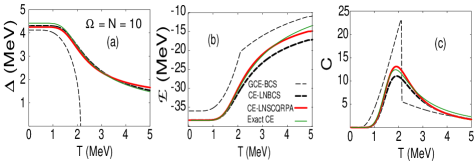
Figure 1: (Color online) Pairing gap $\Delta$, total energy ${\cal E}$ and heat capacity $C$ as functions of $T$ obtained within the Richardson model for $N=$10 with $G$=1 MeV. The thin dashed, thick dashed, thick solid, and thin solid lines denote the GCE-BCS, CE-LNBCS, CE-LNSCQRPA and exact CE results, respectively  .

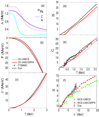
Figure 2: (Color online) Pairing gap $\Delta$, free energy $F$, excitation energy ${\cal E}^{*}$, heat capacity $C$, CE and MCE entropies $S$ as functions of $T$ for ⁵⁶Fe. In (a), the solid and dash-dotted lines denote the neutron and proton gaps, respectively, with the thin and thick lines corresponding to CE-LNBCS and CE-LNSCQRPA results, respectively. In (b) – (e), the thin and solid lines denote the CE-LNBCS and CE-LNSCQRPA results, whereas the dashed line and the full squares connected by solid line stand for the experimental data and the FTSMMC results, respectively. In (f), the MCE entropies obtained within the MCE-LNBCS (circles), MCE-LNSCQRPA (triangles) are plotted vs experimental data (open squares with error bars) .

The proposed approach is tested within a schematic model and applied to describe thermodynamic quantities for a realistic nucleus. For the schematic model, we employ the so-called Richardson (or ladder) model, which consists of $\Omega$ doubly-folded equidistant levels with the single-particle energies chosen as $\epsilon_{j}=j-(\Omega+1)/2$ MeV. The model is half-filled, i.e. $N=\Omega$. As for the realistic nucleus, we employ the axially deformed Woods-Saxon single-particle spectra for Fe⁵⁶ nucleus with the depth of the central potential $V=V_{0}[1\pm k(N-Z)/(N+Z)]$, where $V_{0}=$ 51.0 MeV, $k=$ 0.86, the diffuseness $a$=0.67 fm, $r_{0}$=1.27 fm WS , the deformation parameter $\beta_{2}=$ 0.244 SMMC1 , and the spin-orbit strength $\lambda=$ 35.0.

Shown in Fig. 1 are the pairing gaps $\Delta$, total energies ${\cal E}$ and heat capacities $C$ obtained within the GCE-BCS, CE-LNBCS, CE-LNSCQRPA as well as the exact CE for the Richardson model with $N=$10 and $G$ = 1 MeV. The figure clearly shows that the CE-LNSCQRPA results (thick solid lines) nearly coincide with the exact CE (thin solid lines) for all thermodynamic quantities under consideration. A slight difference between the CE-LNSCQRPA results and the exact ones at very high $T$ occurs because the CE-LNSCQRPA includes only the low-lying excited states in the ensemble. These states are known to be important in low and medium temperature regions. At very high $T$, one needs to include high-lying excited states into the ensemble as well. The same feature is seen from the results obtained for other systems with different $N$ and $G$. The results obtained within the CE-LNBCS (thick dashed lines) are a bit off from the exact ones but, as compared to the predictions by the GCE-BCS (thin dashed lines), they still offer much better agreement with the exact solutions. The most interesting feature is that neither the pairing gaps obtained within the CE-LNBCS nor those obtained within the CE-LNSCQRPA collapse at the critical temperature $T_{C}$ as predicted by the GCE-BCS, but they all monotonously decrease with increasing $T$, just like the exact CE gap. Consequently, the sharp peak in the heat capacity, which is the signature of SN phase transition, is smoothed out within these approaches. This feature implies that the CE-LNBCS and CE-LNSCQRPA include the effects of quantal and thermal fluctuations, which are neglected in the GCE-BCS. Moreover, it also suggests that, if any exact PNP method at finite $T$ could bring the GCE-BCS to the CE-BCS, the results obtained within this projected CE-BCS should have the same qualitative behavior as the CE-LNBCS results presented in present article with a nonvanishing gap.

The pairing gap, free energy, excitation energy, heat capacity and entropy in ⁵⁶Fe nucleus are displayed in Fig. 2. In order to have a consistent comparison with the recent experimental data in EXP as well as the FTSMMC results for these quantities, we employ the same configurations proposed in SMMC2 , namely the CE-LNBCS and CE-LNSCQRPA are calculated within the complete $pf+0g_{9/2}$ major shell. The results obtained within this shell are then combined with those obtained within the independent-particle model (IPM) by using Eq. (15) of SMMC2 , where $Z^{{}^{\prime}}_{\nu,tr}$ in the present case is the CE-LNBCS or CE-LNSCQRPA partition function, whereas $Z^{{}^{\prime}}_{sp}$ and $Z^{{}^{\prime}}_{sp,tr}$ are the CE partition functions obtained within the IPM for full (from bottom to $h_{11/2}$ orbital) and truncated (from $f_{7/2}$ to $h_{11/2}$ orbitals) model spaces, respectively (The width of resonance single-particle states is neglected for simplicity). The parameter $G$ is adjusted so that the pairing gaps for protons (Z) and neutrons (N) obtained within the LNBCS at $T=$ 0 reproduce the experimental values, namely $\Delta_{Z}\simeq$1.57 MeV and $\Delta_{N}\simeq$ 1.36 MeV EXP . It is clear from this figure that the CE-LNSCQRPA results agree quite well with the experimental data, which are also deducted from the CE. The small difference between the CE-LNSCQRPA results and experimental data at high $T$ is probably due to the fact that latter have been extracted from the experimental level density rather than being obtained from direct measurements. The level density, however, cannot be measured at high excitation energy $E^{*}>$ 10 MeV, but has been instead obtained from the back-shifted Fermi gas (BSFG) formula (see e.g. Eq. (2) of EXP ), assuming a zero pairing gap in this region of excitation energy. As we can see now, this approximation is rather crude because the pairing gap is always finite even at high $E^{*}>$ 10 MeV (or $T>T_{C}$) because of thermal fluctuations. This is demonstrated in Fig. 2 (a), which clearly shows that, at $T>$ 1.5 MeV, which corresponds to $E^{*}>$ 10 MeV, the neutron and proton gaps are still finite. This feature puts the use of BSFG formula to extrapolate the measured level density to high $E^{*}$ under question. As regards the heat capacity obtained from the experimental data plus BSFG [Fig. 2 (e)], it only shows an oscillation rather than a peak or even an S shape in the temperature region around $T_{C}$, whereas all CE-LNBCS, CE-LNSCQRPA as well as FTSMMC results predict a bump in this region. The absence of a bump at $T\sim T_{C}$ in the experimentally extracted heat capacity for ⁵⁶Fe also seems to contradict those obtained for nuclei in rare-earth region by using the same method, where a clear S shape or even a broad bump has been seen Kaneko . Regarding the difference shown in Fig. 2 (e) between the FTSMMC results and ours at high $T$, it might come from the absence of quadrupole interaction in our calculations. It has been well-known that the multipole interactions, in particular the quadrupole force, which is important for quadrupole deformation, can have significant effects on the nuclear level density at moderate and high temperatures (See Fig. 8 and Table 1 in Ref.  DangZP ). Fluctuations of other degrees of freedom such as nuclear shapes due to rotation may also play an important role. Most probably these effects will show up at high temperatures and angular momenta, which are considered neither in the experimental data for ⁵⁶Fe that we use nor within the present framework of our model.

A genuine thermodynamic observable is the MCE entropy at low $E^{*}$ because it is calculated directly from the measured level density (See e.g. Eq. (3) of EXP ). Shown in Fig. 2 (f) are the MCE entropies obtained within the MCE-LNBCS and MCE-LNSCQRPA using the Boltzmann’s definition with $\delta{\cal E}$ = 1 MeV versus the experimental data. It is seen that the MCE-LNSCQRPA entropy not only offers the best fit to the experimental data but also predicts the results up to higher $E^{*}>$ 10 MeV.

In summary, we have proposed two approximations, which embed the solutions of the BCS and SCQRPA with Lipkin-Nogami PNP at $T=0$ into the CE and MCE. The proposed approaches are tested within the Richardson model and applied to describe the recent experimentally extracted thermodynamic quantities for ⁵⁶Fe nucleus. The analysis of numerical calculations for the pairing gap, free energy, total energy, heat capacity and entropy shows that the CE-LNSCQRPA predictions are in quite good agreements with the exact results (whenever the latter are available), as well as the recent experimental data. Moreover, this is a microscopic approach that can describe simultaneously and selfconistently all the experimentally extracted quantities, namely the free energy, total energy, heat capacity, and entropy within both CE and MCE treatments. To our knowledge, this is the first time that the recent experimental MCE entropy EXP has been successfully described by a consistent microscopic theory. It also shows that the SN phase transition predicted by the conventional GCE-BCS theory is smoothed out even within the CE-LNBCS calculations due to the effects of quantal and thermal fluctuations, leading a nonvanishing pairing gap. The results of the present study put under question the use of BSFG formula to extrapolate the measured level density to high excitation energy. The merit of the present approach resides in its simplicity and its feasibility in the application to larger finite systems, where the exact matrix diagonalization and/or solving the Richardson equation are impracticable to find all eigenvalues, whereas the FTSMMC method is time consuming.

The authors thank Peter Schuck (Orsay) for fruitful discussions. NQH is a Nishina Memorial Fellow at RIKEN. The numerical calculations were carried out using the FORTRAN IMSL Library by Visual Numerics on the RIKEN Integrated Cluster of Clusters (RICC) system.

References

- (1) J. Bardeen, L. Cooper, and Schrieffer, Phys. Rev. 108, 1175 (1957).
- (2) L.G. Moretto, Phys. Lett. B 40, 1 (1972); A.L. Goodman, Phys. Rev. C 29, 1887 (1984); J.L. Egido, P. Ring, S. Iwasaki, and H.J. Mang, Phys. Lett. B 154, 1 (1985).
- (3) R. Rossignoli, P. Ring and N.D. Dang, Phys. Lett. B 297, 9 (1992); N.D. Dang, P. Ring and R. Rossignoli, Phys. Rev. C 47, 606 (1993).
- (4) V. Zelevinsky, B.A. Brown, N. Frazier, and M. Horoi, Phys. Rep. 276, 85 (1996).
- (5) N. Dinh Dang and V. Zelevinsky, Phys. Rev. C 64, 064319 (2001); N. Dinh Dang and A. Arima, Phys. Rev. C 67, 014304 (2003); N.D. Dang and A. Arima, Phys. Rev. C 68, 014318 (2003); N.D. Dang, Nucl. Phys. A 784, 147 (2007).
- (6) N. Dinh Dang and N. Quang Hung, Phys. Rev. C 77, 064315 (2008); N.Q. Hung and N.D. Dang, Phys. Rev. C 78, 064315 (2008).
- (7) N.Q. Hung and N.D. Dang, Phys. Rev. C 79, 054328 (2009).
- (8) R.W. Richardson, Phys. Lett. 3, 277 (1963); Ibid. 14, 325 (1965); A. Volya, B.A. Brown, and V. Zelevinsky, Phys. Lett. B 509 (2001) 37.
- (9) T. Sumaryada and A. Volya, Phys. Rev. C 76, 024319 (2007).
- (10) S. Liu and Y. Alhassid, Phys. Rev. Lett 87, 022501 (2001).
- (11) Y. Alhassid, G. F. Bertsch, and L. Fang, Phys. Rev. C 68, 044322 (2003).
- (12) K. Tanabe and H. Nakada, Phys. Rev. C 71, 024314 (2005); H. Nakada and K. Tanabe, Phys. Rev. C 74, 061301(R) (2006).
- (13) R. Rossignoli and P. Ring, Ann. Phys. (NY) 235, 350 (1994), R. Rossignoli, P. Ring, and N. D. Dang, Phys. Lett. B297, 9 (1992).
- (14) H. J. Lipkin, Ann. Phys. (NY) 9 272 (1960); Y. Nogami, Phys. Lett. 15 4 (1965).
- (15) N.Q. Hung and N.D. Dang, Phys. Rev. C 76, 054302 (2007); Ibid. 77, 029905(E) (2008).
- (16) S. Cwiok et al., Comput. Phys. Commun. 46, 379 (1987).
- (17) E. Algin et al., Phys. Rev. C 78, 054321 (2008).
- (18) A. Schiller et al., Phys. Atom. Nucl. 64, 1186 (2001); K. Kaneko et al., Phys. Rev. C 74, 024325 (2006).
- (19) N. Dinh Dang, Z. Phys. A 335, 253 (1990).