Semi-inclusive bottom-Higgs production at LHC:
The complete one-loop electroweak effect in the MSSM

Abstract

We present the first complete calculation of the one-loop electroweak effect in the process of semi-inclusive bottom-Higgs production at LHC in the MSSM. The size of the electroweak contribution depends on the choice of the final produced neutral Higgs boson, and can be relevant, in some range of the input parameters. A comparison of the one-loop results obtained in two different renormalization schemes is also performed, showing a very good NLO scheme independence. We further comment on two possible, simpler, approximations of the full NLO result, and on their reliabilty.

I Introduction

It is a well known fact that $\tan\beta$ enhanced Yukawa coupling in the Minimal Supersymmetryc Standard Model (MSSM) could favour the Higgs production in association with bottom quarks, contrarily to the Standard Model (SM) case, where the Higgs production is dominated by top-Higgs coupling.

Due to its relevance as a possible channel for the Higgs discovery, in the last few years the associated bottom-Higgs production has been extensively studied in the literature. Depending on the choice of the flavour-scheme in the partonic description of the initial state and on the identified final state, one can consider a number of different partonic sub-processes for $\mathcal{H}^{0}+b_{jets}$ production: while the choice of the 4 versus 5 flavour scheme is mainly theoretically motivated, resulting in a reordering of the perturbative expansion Campbell:2004pu , the requirement of a minimum number of tagged $b$ in the final state is physically relevant in the signal extraction. Assuming the 5-flavour scheme (which ensures a better convergence of the perturbative series resumming large logarithms in the bottom PDF), one can consider three different types of production processes, depending on the required final states: the exclusive one where both bottom jets are tagged ($b\bar{b}\mathcal{H}^{0}$ final state), the semi-inclusive one where only one bottom quark is tagged ($b\mathcal{H}^{0}$), and the inclusive one where no bottom quark jets are tagged. While the inclusive process has a larger cross section EX-NLOQCD , the semi-inclusive with a high $p_{b,T}$ bottom in the final state is experimentally more appealing SI-NLOQCD1 .

The relative weights of the partonic processes ($b\bar{b}\to\mathcal{H}^{0}$, $bg\to b\mathcal{H}^{0}$, $gg\to b\bar{b}\mathcal{H}^{0}$) are analyzed in EX-NLOQCD , where also the $\alpha_{s}$ corrections (NLO) to the leading sub-process $b\bar{b}\to\mathcal{H}^{0}$ are computed. The NNLO order in QCD ($\alpha_{s}^{2}$) for the same sub-process is calculated in EX-NNLOQCD , while the electroweak (SM and MSSM) and SUSY-QCD NLO corrections have been computed in I-EW , showing that the size of electroweak corrections can be comparable, for large $\tan\beta$, with that of the strong ones.

The associated semi-inclusive production process ($b\mathcal{H}^{0}$ final state) is analyzed at the NLO in QCD in SI-NLOQCD1 and SI-NLOQCD2 , while the effect of the SUSY QCD is given in SI-SQCD . Very recently, Dawson and Jaiswal have also computed, for the Standard Model process $bg\to b\,h_{SM}$, the one-loop weak corrections dj10 .

Finally, the exclusive process, where two bottom jets are tagged in the final state, is considered at the NLO in QCD in Campbell:2004pu , djrw06 , Dittmaier:2003ej and Dawson:2003kb . The leading Yukawa corrections for this partonic process are considered in EX-EW and SUSY QCD effects have also been computed in EX-SQCD .

Our paper is strongly motivated by the possible relevance of the associated bottom-Higgs production in the experimental search of the Higgs at the LHC; moreover, as stressed in I-EW , the susy one-loop ew effects (for the inclusive process) can be sizable and they can be safely accounted by an improved born approximation. Therefore the spirit of our computation is twofold: on the one hand we provide for the first time the complete NLO EW corrections for the semi-inclusive process, including also the overall QED effect, that was not computed by dj10 , and on the other hand we can perform a further and independent test on the validity and limits of the improved born approximation in different scenarios. Our calculations have been performed in two different ($\overline{\rm DR}$ and DCPR) renormalization schemes: as expected the final one-loop results are, within at most a relative few percent difference, the same in the two frames; however, the $\overline{\rm DR}$ scheme appears to be the one where the perturbative effect is numerically mostly more under control. Therefore we shall discuss our results in this frame, showing in various figures the dependence of the different observables on the choice of the input parameters. We have finally compared the results obtained with the full electroweak computation with those obtained within a commonly used approximation scheme. This will be done in the final part of our paper, which is organized as follows: Section II contains a general concentrated discussion of the actual derivation of the theoretical formulae (a part of which has been shifted in a technical Appendix B) to be used for the calculation of the various observables. Section III and IV contains our numerical results, that are briefly discussed in the final Section V.

II Kinematics and Amplitude of the process $bg\to b\mathcal{H}^{0}$

II.1 Kinematics

At lowest order there is only one partonic${}^{\mbox{\tiny{\ref{foot:pb}}}}$ channel leading to bottom-Higgs production

$$b(p_{b})~{}g(p_{g})\to b(p^{\prime}_{b})~{}\mathcal{H}^{0}(p_{\mathcal{H}^{0}})$$ (1)

where $\mathcal{H}^{0}$ is one of the three MSSM neutral Higgs bosons ($h^{0},\,H^{0},\,A^{0}$). In the partonic center of mass frame the momenta of the particles read

$$p_{b}=(E_{b};0,0,p), p_{g}=(p;0,0,-p),$$

$$p^{\prime}_{b}=(E^{\prime}_{b};p^{\prime}\sin\theta,0,p^{\prime}\cos\theta), p_{\mathcal{H}^{0}}=(E_{\mathcal{H}^{0}};-p^{\prime}\sin\theta,0,-p^{\prime}\cos\theta).$$ (2)

The Mandelstam variables are defined as

$$s=(p_{g}+p_{b})^{2},~{}~{}t=(p_{b}-p^{\prime}_{b})^{2},~{}~{}u=(p_{g}-p^{\prime}_{b})^{2}.$$ (3)

For later convenience we define two momenta $q$ and $q^{\prime}$ as follows

$$q=p_{b}+p_{g},~{}~{}~{}~{}~{}q^{\prime}=p^{\prime}_{b}-p_{g}$$

II.2 Born and one-loop amplitudes

We denote the $\mathcal{O}(\alpha^{a}_{s}\alpha^{b})$ contribution to the amplitude (differential cross section) of the process $X$ as $\mathcal{M}^{a,b}_{X}$ ($d\sigma^{ab}_{X}$). The Born terms result from the $s$- and $u$-channel $b$ quark exchange of Figure 1. The color stripped tree-level amplitude reads as follows

$$\mathcal{M}^{1/2,1/2}_{bg\to b\mathcal{H}^{0}} = -\left({g_{s}\over s-m^{2}_{b}}\right)\bar{u}^{\prime}_{b}(\lambda^{\prime}_{b})[c^{L}(bb\mathcal{H}^{0})P_{L}+c^{R}(bb\mathcal{H}^{0})P_{R}](q\hskip-5.97527pt/+m_{b})\epsilon_{g}\hskip-9.38945pt/(\mu)u_{b}(\lambda_{b}),$$ (4)

$$-\left({g_{s}\over u-m^{2}_{b}}\right)\bar{u}^{\prime}_{b}(\lambda_{b}^{\prime})\epsilon_{g}\hskip-9.38945pt/(\mu)(q^{\prime}\hskip-8.2511pt/+m_{b})[c^{L}(bb\mathcal{H}^{0})P_{L}+c^{R}(bb\mathcal{H}^{0})P_{R}]u_{b}(\lambda_{b}),$$

where $\lambda_{b}$, ($\lambda^{\prime}_{b}$) is the helicity of the initial (final) bottom quark while $\mu$ is the polarization of the gluon. $u_{b}(\lambda_{b})$ [$u^{\prime}_{b}(\lambda^{\prime}_{b})$] is the spinor of the initial [final] bottom quark, $\epsilon_{g}(\mu)=(0;\mu/\sqrt{2},-~{}i/\sqrt{2},0)$ is the gluon polarization vector and $P_{R,L}=(1\pm\gamma^{5})/2$ are the chirality projectors. The relevant couplings $c^{\eta}(bb\mathcal{H}^{0})$ ($\eta=L,R$) are defined as

$$c^{\eta}(bbH^{0})=-~{}\left({em_{b}\over 2s_{W}M_{W}}\right){\cos\alpha\over\cos\beta}, c^{\eta}(bbh^{0})=\left({em_{b}\over 2s_{W}M_{W}}\right){\sin\alpha\over\cos\beta}$$

$$c^{L}(bbA^{0})=-i\left({em_{b}\over 2s_{W}M_{W}}\right)\tan\beta, c^{R}(bbA^{0})=c^{L*}(bbA^{0})~{}.$$ (5)

We factorize out of the gluon couplings the colour matrix element $\lambda^{a}/2$. The sum over colors leads to a factor

$$\sum_{a=1}^{8}\mbox{tr}\left\{\frac{\lambda^{a}}{2}~{}\frac{\lambda^{a}}{2}\right\}=4$$ (6)

that multiplies the squared amplitude.
The generic helicity amplitude can be decomposed on a set of eight forms factors $J^{k\eta}$ ($\eta=L,R$) as follows

$$\mathcal{M}^{1/2,1/2}_{bg\to b\mathcal{H}^{0}}=\bar{u}^{\prime}_{b}(\lambda^{\prime}_{b})\left(\sum_{k=1}^{4}\sum_{\eta=L,R}J^{k\eta}N^{k\eta}_{bg\to b\mathcal{H}^{0}}\right)u_{b}(\lambda_{b}),$$ (7)

where

$$J_{1\eta}=p_{g}\hskip-9.95863pt/~{}\epsilon_{g}\hskip-9.38945pt/(\mu)P_{\eta},~{}~{}~{}J_{2\eta}=(\epsilon_{g}(\mu).p^{\prime}_{b})P_{\eta},~{}~{}~{}J_{3\eta}=\epsilon_{g}\hskip-9.38945pt/(\mu)P_{\eta},~{}~{}~{}J_{4\eta}=(\epsilon_{g}(\mu).p^{\prime}_{b})p_{g}\hskip-9.95863pt/~{}P_{\eta}.$$ (8)

The only non-zero scalar functions at the tree level are $N^{1\eta}_{bg\to b\mathcal{H}^{0}}$ and $N^{2\eta}_{bg\to b\mathcal{H}^{0}}$. They read as follows

$$N^{1\eta}_{bg\to b\mathcal{H}^{0}}=-g_{s}{c^{\eta}(bb\mathcal{H}^{0})\over s-m^{2}_{b}}-g_{s}{c^{\eta}(bb\mathcal{H}^{0})\over u-m^{2}_{b}},~{}~{}~{}N^{2\eta}_{bg\to b\mathcal{H}^{0}}=-2g_{s}{c^{\eta}(bb\mathcal{H}^{0})\over u-m^{2}_{b}}$$ (9)

The one-loop electroweak virtual contributions arise from self energy, vertex and box diagrams. Counterterms for the various bottom quarks lines, for the $\mathcal{H}^{0}$ line, and for the $bb\mathcal{H}^{0}$ coupling constants have to be considered as well. The corresponding diagrams can be read off from Fig 2, 3.
All these contributions have been computed using the usual decomposition in terms of Passarino-Veltman functions and the complete amplitude has been implemented in a C++ numerical code.

II.3 Renormalization

In order to cancel the ultraviolet (UV) divergences the Higgs sector and the bottom sector have to be renormalized at $\mathcal{O}(\alpha)$. The expressions of the counterterms entering our calculation are collected in Appendix B.

Higgs sector
As anticipated we performed the calculation using two different renormalization schemes: the $\overline{\mbox{DR}}$ scheme Frank:2006yh is defined by the following renormalization conditions

$$\delta Z^{\overline{\mbox{\tiny DR}}}_{H_{1}} = -\left[\,\mbox{Re}\frac{\partial\Sigma_{H^{0}}(k^{2})}{\partial k^{2}}|_{k^{2}=M^{2}_{H^{0}},\alpha=0}\,\right]_{\mbox{\tiny div}}\,$$

$$\delta Z^{\overline{\mbox{\tiny DR}}}_{H_{2}} = -\left[\,\mbox{Re}\frac{\partial\Sigma_{h^{0}}(k^{2})}{\partial k^{2}}|_{k^{2}=M_{h^{0}},\alpha=0}\,\right]_{\mbox{\tiny div}}\,$$

$$\delta T_{h^{0}} = -T_{h^{0}}\,$$

$$\delta T_{H^{0}} = -T_{H^{0}}\,$$

$$\delta M_{A^{0}}^{2} = \mbox{Re}\Sigma_{A^{0}}(M_{A^{0}}^{2})-M_{A^{0}}^{2}\Sigma^{\prime}_{A^{0}}(M_{A^{0}}^{2})$$

$$\delta\tan\beta^{\overline{\mbox{\tiny DR}}} = \frac{1}{2}\left(\delta Z^{\overline{\mbox{\tiny DR}}}_{H_{2}}-\delta Z^{\overline{\mbox{\tiny DR}}}_{H_{1}}\right)\tan\beta.$$ (10)

$\delta Z^{\overline{\mbox{\tiny DR}}}_{H_{i}}$ define the wave function renormalization costant of the Higgs field $H_{i}$, the third and fourth line fix the tadpole renormalization and the last one the $\tan\beta$ renormalization constant. $[\mathcal{A}]_{\mbox{\tiny div}}$ means keeping the UV divergent part of $\mathcal{A}$, discarding the finite contribution. In the DCPR scheme Dabelstein:1994hb ; Chankowski:1992er the independent parameters are the same, and the renormalization conditions of the Higgs wavefunctions change as follows

$$\delta Z^{\mbox{\tiny DCPR}}_{H_{1}} = -\mbox{Re}\frac{\partial\Sigma_{A^{0}}(k^{2})}{\partial k^{2}}|_{k^{2}=M^{2}_{A^{0}}}-\frac{1}{\tan\beta M_{Z}}\mbox{Re}\Sigma_{A^{0}Z}(M^{2}_{A^{0}})\,$$

$$\delta Z^{\mbox{\tiny DCPR}}_{H_{2}} = -\mbox{Re}\frac{\partial\Sigma_{A^{0}}(k^{2})}{\partial k^{2}}|_{k^{2}=M^{2}_{A^{0}}}+\frac{\tan\beta}{M_{Z}}\mbox{Re}\Sigma_{A^{0}Z}(M^{2}_{A^{0}})\,$$

$$\delta T_{h^{0}} = -T_{h^{0}}\,$$

$$\delta T_{H^{0}} = -T_{H^{0}}\,$$

$$\delta M_{A^{0}}^{2} = \mbox{Re}\Sigma_{A^{0}}(M_{A^{0}}^{2})-M_{A^{0}}^{2}\Sigma^{\prime}_{A^{0}}(M_{A^{0}}^{2})$$

$$\delta\tan\beta^{\mbox{\tiny DCPR}} = \frac{1}{2}\left(\delta Z^{\mbox{\tiny DCPR}}_{H_{2}}-\delta Z^{\mbox{\tiny DCPR}}_{H_{1}}\right)\tan\beta$$ (11)

We choose to impose on-shell (OS) condition for the mass of CP-odd $A^{0}$ Higgs in both schemes.

The renormalization constants of the Higgs bosons wavefunctions and of the $c^{\eta}(bb\mathcal{H}^{0})$ couplings can be written in terms of the of the renormalization constants defined above. Their explicit expression is given in Appendix A.

Bottom sector
The mass of the bottom and its wavefunction renormalization function is fixed in the on-shell scheme:

$$\delta m^{\mbox{\tiny OS}}_{b} = \frac{1}{2}m_{b}\left[\mbox{Re}\Sigma_{{b}_{L}}(m_{b}^{2})+\mbox{Re}\Sigma_{{b}_{R}}(m_{b}^{2})+2\mbox{Re}\Sigma_{{b}_{S}}(m_{b}^{2})\right],$$ (12)

$$\delta Z^{L}_{b} = -\mbox{Re}\Sigma_{{b}_{L}}(m_{b}^{2})-m_{b}^{2}\frac{\partial}{\partial k^{2}}\mbox{Re}\left[\Sigma_{{b}_{L}}(k^{2})+\Sigma_{{b}_{R}}(k^{2})+2\Sigma_{{b}_{S}}(k^{2})\right]|_{k^{2}=m_{b}^{2}},$$

$$\delta Z^{R}_{b} = -\mbox{Re}\Sigma_{{b}_{R}}(m_{b}^{2})-m_{b}^{2}\frac{\partial}{\partial k^{2}}\mbox{Re}\left[\Sigma_{{b}_{L}}(k^{2})+\Sigma_{{b}_{R}}(k^{2})+2\Sigma_{{b}_{S}}(k^{2})\right]|_{k^{2}=m_{b}^{2}},$$

where the bottom self energies are defined according to following Lorentz decomposition:

$$\Sigma_{b}(p)=\makebox[0.86108pt][l]{$p$}/P_{L}\Sigma_{{b}_{L}}(p^{2})+\makebox[0.86108pt][l]{$p$}/P_{R}\Sigma_{{b}_{R}}(p^{2})+m_{b}\Sigma_{{b}_{S}}(p^{2})\;.$$ (13)

The bottom masses in the Yukawa couplings are treated completely at the electroweak level, with OS or $\overline{\mbox{DR}}$ renormalization conditions respectively in the two schemes. Resummation of large logarithms from the running of the bottom mass suggests to trade bottom mass appearing in the couplings with an effective bottom mass,  Heinemeyer:2004xw . The resummation of the $(\alpha_{s}\tan\beta)^{n}$ contributions can be achieved modifying the tree level relation between the bottom Yukawa coupling and the bottom mass: the bottom mass of the couplings, which is related to the bottom Yukawa coupling, is replaced by an effective mass, (e. g. in the $\overline{\mbox{DR}}$ scheme)

$$m^{\overline{\mbox{\tiny DR}}}_{b}\to\overline{m}^{\overline{\mbox{\tiny DR}}}_{b}=\frac{m^{\overline{\mbox{\tiny DR}}}_{b}}{1+\Delta_{b}}$$ (14)

where $\Delta_{b}$ is given by

$$\Delta_{b} = \frac{2}{3}\frac{\alpha_{s}}{\pi}\,M_{\tilde{g}}\,\mu\,\tan\beta\;I(M_{\tilde{b}_{1}},M_{\tilde{b}_{2}},M_{\tilde{g}})$$ (15)

$$I(a,b,c) = \frac{-1}{(a^{2}-b^{2})(b^{2}-c^{2})(c^{2}-a^{2})}\left(a^{2}b^{2}\ln\frac{a^{2}}{b^{2}}+b^{2}c^{2}\ln\frac{b^{2}}{c^{2}}+c^{2}a^{2}\ln\frac{c^{2}}{a^{2}}\right).$$

Moreover, the $b\bar{b}H_{1}$ coupling is dynamically generated at $\mathcal{O}(\alpha_{s})$ and can be enhanced if $\tan\beta$ is large. This effect can be included modifying the $c^{\eta}(bb\mathcal{H}^{0})$ couplings. The actual effect of this modification and of the bottom mass resummation, Eq: (14), is to substitute the $c^{\eta}(bb\mathcal{H}^{0})$ couplings in Eq. (5) as follows

$$c^{\eta}(bbh^{0}) \to \frac{c^{\eta}(bbh^{0})}{m_{b}}\times\overline{m}^{\overline{\mbox{\tiny DR}}}~{}\left(1-\frac{\Delta_{b}}{\tan\beta\tan\alpha}\right)$$

$$c^{\eta}(bbH^{0}) \to \frac{c^{\eta}(bbH^{0})}{m_{b}}\times\overline{m}^{\overline{\mbox{\tiny DR}}}~{}\left(1+\frac{\Delta_{b}\tan\alpha}{\tan\beta}\right)$$

$$c^{\eta}(bbA^{0}) \to \frac{c^{\eta}(bbA^{0})}{m_{b}}\times\overline{m}^{\overline{\mbox{\tiny DR}}}~{}\left(1-\frac{\Delta_{b}}{\tan^{2}\beta}\right).$$ (16)

We have checked the cancellation of the UV divergences among counterterms, self-energies and triangles. This cancellation occurs separately inside 8 sectors, i.e. $s$-channel “initial” triangles with chirality L or R, $s$-channel “final” L or R, $u$-channel up triangles (L or R) and $u$-channel down triangles (L or R). The Box diagrams are UV finite.

II.4 QED radiation

The infrared (IR) singularities affecting the virtual contributions are cancelled including the bremsstrahlung of real photons at $\mathcal{O}(\alpha_{s}\alpha^{2})$,

$$b(p_{b})~{}g(p_{g})\to~{}b(p^{\prime}_{b})~{}\mathcal{H}^{0}(p_{\mathcal{H}^{0}})~{}\gamma(p_{\gamma})\,,$$ (17)

arising from the diagrams in Figure 4. This contribution has been computed using FeynArts Kublbeck:1990xc and FormCalc Hahn:1998yk . The integral over the photon pase space is IR divergent in the soft-photon region, i.e. for $p^{0}_{\gamma}\to 0$. The IR divergences are regularized within mass regularization, giving a small mass $m_{\gamma}$ to the photon. The phase space integration has been performed using the phase space slicing method. This method introduces a fictitious separator $\Delta E$ and restricts the numerical phase space integration in the region characterized by $p_{\gamma}>\Delta E$. The integral over the region $p_{\gamma}<\Delta E$ is performed analytically in the eikonal approximation Baier:1973ms .

Large collinear logarithms containing the bottom mass can be re-absorbed into the redefinition of the parton distribution function (PDF) of the bottom $f_{b}(x,\mu)$. In the $\overline{\mbox{MS}}$ (DIS) factorization scheme this is achieved performing the substitution Baur:1998kt

$$f_{b}(x,\mu) \to f_{b}(x,\mu)\left\{1-\frac{\alpha}{\pi}e^{2}_{b}\left[1-\ln\delta_{s}-\ln\delta^{2}_{s}+\left(\ln\delta_{s}+\frac{3}{4}\right)\ln\left(\frac{\mu^{2}}{m_{b}^{2}}\right)-\frac{1}{4}\lambda_{\mbox{\tiny FC}}\kappa_{1}\right]\right\}$$ (18)

$$- \frac{\alpha}{2\pi}e^{2}_{b}\int_{x}^{1-\delta_{s}}\;\frac{dz}{z}\;f_{b}\left(\frac{x}{z},\mu\right)\left[\frac{1+z^{2}}{1-z}\ln\left(\frac{\mu^{2}}{m^{2}_{b}}\frac{1}{(1-z)^{2}}\right)-\frac{1+z^{2}}{1-z}+\lambda_{\mbox{\tiny FC}}\kappa_{2}\right],$$

and setting $\lambda_{\mbox{\tiny FC}}=0$ ($\lambda_{\mbox{\tiny FC}}=1$). $\mu$ is the factorization scale, $\delta_{s}=2\Delta E/\sqrt{s}$, while $e_{b}$ is the bottom charge. $\kappa_{1}$ and $\kappa_{2}$ are defined as follows,

$$\kappa_{1} = 9+\frac{2}{3}\pi^{2}+3\ln\delta_{s}-2\ln^{2}\delta_{s},$$

$$\kappa_{2} = \frac{1+z^{2}}{1-z}\ln\left(\frac{1-z}{z}\right)-\frac{3}{2}\frac{1}{1-z}+2z+3.$$ (19)

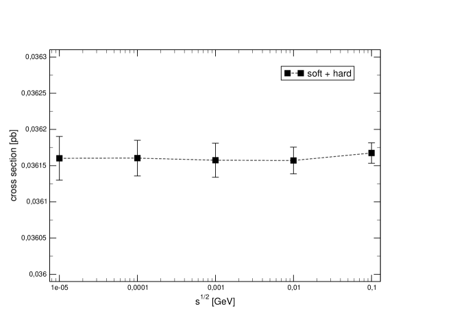
Figure 5: $A^{0}$ production: dependence of the $\mathcal{O}(\alpha)$ soft+virtual, hard, and total sum corrections on the separator $\Delta E$

We tested numerically the cancellation of IR divergences, the independence of our results of $m_{\gamma}$ (in the sum of the soft and virtual part) and of the separator $\Delta E$ (see Figures 5, 6, 7).

II.5 Total cross sections

Including the finite wave function renormalization for the Higgs field we obtain the following expressions for the tree-level differential partonic cross section of the processes we are considering,

$$d\hat{\sigma}^{1,1}_{bg\to b\mathcal{H}^{0}}=\frac{\beta^{\prime}\,d\cos\theta}{768\,\pi\,s\,\beta}~{}Z_{\mathcal{H}^{0}}~{}\left|\mathcal{M}^{1/2,1/2}_{bg\to b\mathcal{H}^{0}}\right|^{2}$$ (20)

where $\beta=2p/\sqrt{s}$, $\beta^{\prime}=2p^{\prime}/\sqrt{s}$, and $s$ is the Mandelstam variable defined in Eq. (3); the NLO-EW contribution to the differential cross section reads as follows

$$d\hat{\sigma}^{1,2}_{bg\to bh^{0}} = \frac{\beta^{\prime}\,d\cos\theta}{768\,\pi\,s\,\beta}~{}Z_{h^{0}}\Bigg{\{}\left|1-Z_{h^{0}H^{0}}\frac{\cos\alpha}{\sin\alpha}\right|^{2}~{}\left|\mathcal{M}^{1/2,1/2}_{bg\to bh^{0}}\right|^{2}$$

$$+ 2~{}\mbox{Re}\mathcal{M}^{1/2,1/2}_{bg\to bh^{0}}\left(\mathcal{M}^{1/2,3/2}_{bg\to bh^{0}}\right)^{*}\Bigg{\}}-d\hat{\sigma}^{1,1}_{bg\to bh^{0}},$$

$$d\hat{\sigma}^{1,2}_{bg\to bH^{0}} = \frac{\beta^{\prime}\,d\cos\theta}{768\,\pi\,s\,\beta}~{}Z_{H^{0}}\Bigg{\{}\left|1-Z_{H^{0}h^{0}}\frac{\sin\alpha}{\cos\alpha}\right|^{2}~{}\left|\mathcal{M}^{1/2,1/2}_{bg\to bH^{0}}\right|^{2}$$

$$+ 2~{}\mbox{Re}\mathcal{M}^{1/2,1/2}_{bg\to bH^{0}}\left(\mathcal{M}^{1/2,3/2}_{bg\to bH^{0}}\right)^{*}\Bigg{\}}-d\hat{\sigma}^{1,1}_{bg\to bH^{0}},$$

$$d\hat{\sigma}^{1,2}_{bg\to bA^{0}} = \frac{\beta^{\prime}\,d\cos\theta}{768\,\pi\,s\,\beta}~{}Z_{A^{0}}\Bigg{\{}2~{}\mbox{Re}\mathcal{M}^{1/2,1/2}_{bg\to bA^{0}}\left(\mathcal{M}^{1/2,3/2}_{bg\to bA^{0}}\right)^{*}\Bigg{\}},$$ (21)

where the Z factors $Z_{h^{0}}$, $Z_{H^{0}}$, $Z_{A^{0}}$, $Z_{h^{0}H^{0}}$, and $Z_{H^{0}h^{0}}$ in the two renormalization schemes we are considering can be found in Frank:2006yh and in Dabelstein:1994hb . The partonic differential cross section for the real photon radiation process reads as follows,

$$d\hat{\sigma}^{1,2}_{bg\to b\mathcal{H}^{0}\gamma}=\frac{1}{4\cdot 24}~{}\frac{d\phi(p^{\prime}_{b},p_{\mathcal{H}^{0}},p_{\gamma})}{2\beta\,s}~{}Z_{\mathcal{H}^{0}}~{}\left|\mathcal{M}^{1/2,1}_{bg\to b\mathcal{H}^{0}\gamma}\right|^{2}$$ (22)

where, according to the notation introduced in Dittmaier:1999mb , $d\phi(p^{\prime}_{b},p_{\mathcal{H}^{0}},p_{\gamma})$ is the three-particles phase space measure. The hadronic differential cross section at $\mathcal{O}(\alpha_{s}\alpha)$ and $\mathcal{O}(\alpha_{s}\alpha^{2})$ reads

$$d\sigma^{1,1}_{PP\to b\mathcal{H}^{0}}(S) = \int_{0}^{1}~{}dx_{1}\int_{0}^{1}~{}dx_{2}\Big{[}f_{b}(x_{1},\mu)f_{g}(x_{2},\mu)+(x_{1}\leftrightarrow x_{2})\Big{]}$$

$$\times d\hat{\sigma}^{1,1}_{bg\to b\mathcal{H}^{0}}(x_{1}x_{2}S)$$

$$d\sigma^{1,2}_{PP\to b\mathcal{H}^{0}(\gamma)}(S) = \int_{0}^{1}~{}dx_{1}\int_{0}^{1}~{}dx_{2}\Big{[}f_{b}(x_{1},\mu)f_{g}(x_{2},\mu)+(x_{1}\leftrightarrow x_{2})\Big{]}$$ (23)

$$\times \Big{[}d\hat{\sigma}^{1,2}_{bg\to b\mathcal{H}^{0}}(x_{1}x_{2}S)+d\hat{\sigma}^{1,2}_{bg\to b\mathcal{H}^{0}\gamma}(x_{1}x_{2}S)\Big{]}$$

respectively. $\sqrt{S}$ is the hadronic center-of-mass energy, while $f_{i}(x_{i},\mu)$ is the parton distribution function of the parton $i$ inside the proton with a momentum fraction $x_{i}$ at the scale $\mu$. For later convenience we define the invariant mass distribution as

$$\frac{d\sigma^{1,1}_{PP\to b\mathcal{H}^{0}}}{d\sqrt{\bar{s}}} = \int_{0}^{1}~{}dx_{1}\int_{0}^{1}~{}dx_{2}\Big{[}f_{b}(x_{1},\mu)f_{g}(x_{2},\mu)+(x_{1}\leftrightarrow x_{2})\Big{]}$$

$$\times d\hat{\sigma}^{1,1}_{bg\to b\mathcal{H}^{0}}(x_{1}x_{2}S)\delta\left(\sqrt{x_{1}x_{2}S}-\sqrt{\bar{s}}\right)$$

$$\frac{d\sigma^{1,2}_{PP\to b\mathcal{H}^{0}}}{d\sqrt{\bar{s}}} = \int_{0}^{1}~{}dx_{1}\int_{0}^{1}~{}dx_{2}\Big{[}f_{b}(x_{1},\mu)f_{g}(x_{2},\mu)+(x_{1}\leftrightarrow x_{2})\Big{]}$$ (24)

$$\times \Big{[}d\hat{\sigma}^{1,2}_{bg\to b\mathcal{H}^{0}}(x_{1}x_{2}S)+d\hat{\sigma}^{1,2}_{bg\to b\mathcal{H}^{0}\gamma}(x_{1}x_{2}S)\Big{]}\delta\left(\sqrt{x_{1}x_{2}S}-\sqrt{\bar{s}}\right)$$

III Numerical Results

The independent input parameters in the MSSM Higgs sector are the $A^{0}$ mass and $\tan\beta$: since we impose the same renormalization condition for $M_{A^{0}}$ only $\tan\beta$ should be converted in the change of scheme, using the one-loop relation:

$$\tan\beta^{\mbox{\tiny DCPR}}=\tan\beta^{\overline{\mbox{\tiny DR}}}+\delta\tan\beta^{\overline{\mbox{\tiny DR}}}-\delta\tan\beta^{\mbox{\tiny DCPR}},$$ (25)

while the OS and $\overline{\rm DR}$ bottom masses $m_{b}^{\mbox{\tiny OS}}$ and $m_{b}^{\overline{\mbox{\tiny DR}}}(\mu)$ are computed starting from $m_{b}^{\overline{\mbox{\tiny MS}}}(m_{b})=4.2$ GeV and following the procedure described in Section 3.2.2 of Heinemeyer:2004xw .

	Scenario	$\;\tan\beta\;$	$\;M_{A^{0}}\;$	$\;M_{\tilde{q},1}\;$	$\;M_{\tilde{q},2}\;$	$\;M_{\tilde{q},3}\;$	$\;M_{1}\;$	$\;M_{2}\;$	$\;M_{\tilde{g}}\;$
	SPP1	$15$	$350$	$350$	$350$	$250$	$90$	$150$	$800$
	SPP2	variable	$250$	$500$	$500$	$400$	$90$	$200$	$800$

Table 1: Inputs parameters for the SUSY scenarios considered in our numerical discussion. $M_{\tilde{q},j}$ is the common value of the breaking parameters in the sector of the squarks belonging to the $j^{\mbox{\tiny th}}$ generation. The dimensionful parameters are given in GeV.

	$\tan\beta\;$	$\;\sigma^{\mbox{\tiny{$\overline{\rm DR}$~{},NLO}}}\;$	$\;\sigma^{\mbox{\tiny{$\overline{\rm DR}$~{},LO}}}\;$	$\;\sigma^{\mbox{\tiny{DCPR,NLO}}}\;$	$\;\sigma^{\mbox{\tiny{DCPR,LO}}}\;$	$\;K^{\mbox{\tiny{$\overline{\rm DR}$~{}}}}\;$	$\;K^{\mbox{\tiny{DCPR}}}\;$	NLO ratio
	10	1.367	1.281	1.371	1.253	1.067	1.093	0.997
	20	5.040	4.784	5.060	4.278	1.053	1.182	0.995
	30	10.601	10.295	10.785	8.505	1.029	1.268	0.98
	40	17.118	17.125	17.615	13.038	0.999	1.350	0.97

Table 2: $A^{0}$ production, SPP₂ spectra: total cross sections [pb], $K$-factors and NLO $\overline{\rm DR}$ /DCPR ratio

	$\tan\beta\;$	$\;\sigma^{\mbox{\tiny{$\overline{\rm DR}$~{},NLO}}}\;$	$\;\sigma^{\mbox{\tiny{$\overline{\rm DR}$~{},LO}}}\;$	$\;\sigma^{\mbox{\tiny{DCPR,NLO}}}\;$	$\;\sigma^{\mbox{\tiny{DCPR,LO}}}\;$	$\;K^{\mbox{\tiny{$\overline{\rm DR}$~{}}}}\;$	$\;K^{\mbox{\tiny{DCPR}}}\;$	NLO ratio
	10	1.338	1.260	1.340	1.234	1.061	1.086	0.998
	20	5.133	4.857	5.099	4.334	1.056	1.176	1.006
	30	10.975	10.461	10.715	8.488	1.049	1.262	1.024
	40	18.613	17.918	17.811	13.248	1.038	1.344	1.045

Table 3: $H^{0}$ production SPP₂ spectra: total cross sections [pb], $K$-factors and NLO $\overline{\rm DR}$ /DCPR ratio

	$\tan\beta\;$	$\;\sigma^{\mbox{\tiny{$\overline{\rm DR}$~{},NLO}}}\;$	$\;\sigma^{\mbox{\tiny{$\overline{\rm DR}$~{},LO}}}\;$	$\;\sigma^{\mbox{\tiny{DCPR,NLO}}}\;$	$\;\sigma^{\mbox{\tiny{DCPR,LO}}}\;$	$\;K^{\mbox{\tiny{$\overline{\rm DR}$~{}}}}\;$	$\;K^{\mbox{\tiny{DCPR}}}\;$	NLO ratio
	10	0.282	0.248	0.282	0.243	1.135	1.156	1.002
	20	0.255	0.254	0.254	0.230	1.005	1.107	1.003
	30	0.228	0.258	0.230	0.217	0.882	1.059	0.988
	40	0.204	0.267	0.213	0.211	0.764	1.012	0.955

Table 4: $h^{0}$ production SPP₂ spectra: total cross sections [pb], $K$-factors and NLO $\overline{\rm DR}$ /DCPR ratio

For the numerical evaluations we used the supersymmetric scenario SPP₁ and a class of points of the parameter space SPP₂, with variable $\tan\beta=10,20,30,40$. The input parameters characterizing these scenarios are summarized in Table 1. The sparticle masses and mixing angles have been obtained with the code FeynHiggs Heinemeyer:1998yj . The one-loop Higgs masses are numerically computed by finding the zero of inverse one-loop propagator matrix determinant

$$[k^{2}-M_{H^{0}}^{2}+\hat{\Sigma}_{H^{0}}(k^{2})][k^{2}-M_{h^{0}}^{2}+\hat{\Sigma}_{h^{0}}(k^{2})]-\hat{\Sigma}^{2}_{H^{0}h^{0}}(k^{2})=0.$$ (26)

Since we require semi-inclusive production (i.e. the bottom quark must be tagged) we impose the following kinematical cuts on the bottom in the final state, limiting the transferred momentum $p_{b,T}>20$ GeV (due to resolution limitations of the hadronic calorimeter) and the rapidity $|y_{b}|<2$ (in order to be able to perform inner tracking). The process we are considering is leading order in QCD. Therefore, analogously to  WjetProd ; Beccaria:2008jq ; Beccaria:2009my , we use a LO QCD PDF set, namely the LO CTEQ6L Pumplin:2002vw . Our choice is justified since the QED effects in the DGLAP evolution equations are known to be small Roth:2004ti . The factorization of the bottom PDF has been performed in the DIS scheme, with factorization scale $\mu=M_{\mathcal{H}^{0}}+m^{\mbox{\tiny OS}}_{b}$.

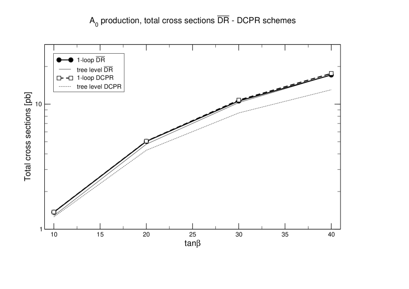
Figure 8: Total LO and NLO cross sections in the $\overline{\rm DR}$ and DCPR schemes, $A^{0}$ production; $M_{A^{0}}=250$ GeV, $p_{b,T}>20$ GeV, $|y_{b}|<2$.

In Figures 8, 9, 10 we show the total cross section for $A^{0},\,H^{0}$ and $h^{0}$ production in the class of supersymmetric scenarios SPP₂, as functions of $\tan\beta$. We present both the results in the $\overline{\rm DR}$ and in the DCPR schemes. The numerical values and the $K$-factors in the two schemes (defined as usual as the ratios $\sigma^{NLO}/\sigma^{LO}$; note that the LO is computed with the resummed/modified SUSY QCD coupling, so our $K$-factors account of the pure electroweak NLO effect), as well as the ratios of the NLO cross sections in the two scheme are reported in Table 2, 3, 4.

As one sees, the values of the total cross sections do coincide in the overall range, apart from small differences of the few percent size for very large $\tan\beta$ values. This confirms our expectation that at the NLO level the two schemes should be equivalent, and also provides an important check of the reliability of our calculations.

Having verified the realistic one-loop equivalence of the two schemes, we have decided to perform our analysis in the $\overline{\rm DR}$ scheme. The main theoretical reasons of our choice have been fully illustrated in schemes . In particular this scheme is known to be generally more stable numerically: our results confirm mainly this expectation but it is worth to note that for $h^{0}$ production both schemes can produce (in different $\tan\beta$ regions) relatively large effects; nevertheless the good agreement between the two schemes leads to suppose that the perturbative expansion is well behaved, and NNLO effects are well under control.

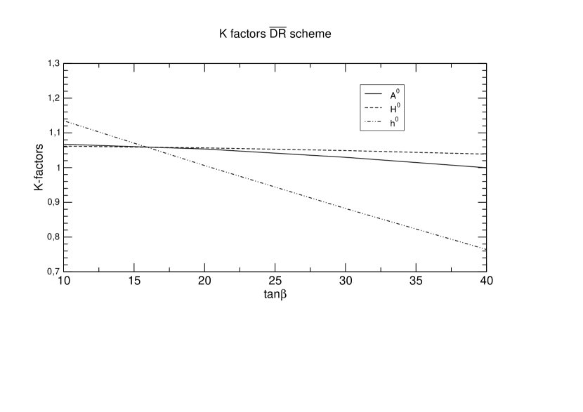
Figure 14: $K$-factors for $A^{0},\,H^{0}$ and $h^{0}$ production, $\overline{\rm DR}$ scheme. $M_{A^{0}}=250$ GeV, $p_{b,T}>20$ GeV, $|y_{b}|<2$.

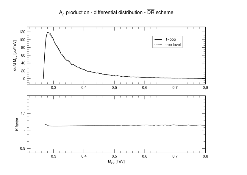
Figure 15: Invariant mass distribution, $A^{0}$ production, $\overline{\rm DR}$ scheme. $M_{A^{0}}=250$ GeV, $\tan\beta=30$ $p_{b,T}>20$ GeV, $|y_{b}|<2$.

Figure 14 shows the $K$-factors for the three Higgs bosons in $\overline{\rm DR}$ as function of $\tan\beta$ while Figures 15, 16, 17 show, for the scenario SPP₂ $\tan\beta=30$, the invariant mass distribution and the relative NLO effect. In the next Figures 18, 19, 20 we again plot the differential distributions for the SPP₁ scenario; the total cross sections for this scenario are reported in Table 5.

	$\mathcal{H}^{0}\;$	$\;\sigma^{\mbox{\tiny{$\overline{\rm DR}$~{},NLO}}}\;$	$\;\sigma^{\mbox{\tiny{$\overline{\rm DR}$~{},LO}}}\;$	$\;K^{\mbox{\tiny{$\overline{\rm DR}$~{}}}}\;$
	$A^{0}$	0.768	0.724	1.060
	$H^{0}$	0.769	0.727	1.056
	$h^{0}$	0.213	0.222	0.961

Table 5: SPP₁ spectrum: total cross sections [pb] for the three Higgs and $\overline{\rm DR}$ $K$-factors

From inspection of the figures, one can draw the following main conclusions:

1. The $K$-factors for $H^{0},A^{0}$ are systematically small for large $\tan\beta$, and would reach a larger size (roughly, 8 %) for small $\tan\beta$ values around 10.

2. The $K$-factor for $h^{0}$ varies drastically with $\tan\beta$, changing from positive values of about 15 % for $\tan\beta$ around 10 to negative values of about 25 % for $\tan\beta$ around 40. These extreme negative and positive values are of a size that cannot be ignored in a dedicated experimental analysis.

These features follow from the THDM structure and the $h^{0}-H^{0}$ mixing where $\alpha$ is close to $\beta-\pi/2$ leading to a $\tan\beta$ enhancement in the $h^{0}$ case but to a $1/\tan\beta$ suppression in the $H^{0},A^{0}$ cases.

This, we believe, is the main message of our calculation: while for sure the QCD NLO are the dominant corrections (of order $20-40\%$ depending on the Higgs mass, see for example SI-NLOQCD1 ), as it was to be expected from the analysis of Dittmaier et al. I-EW , the one-loop electroweak contribution in the semi-inclusive bottom-Higgs production processes must not be a priori considered as negligible.

IV Numerical Approximations

Having performed the calculation of complete one-loop effect on the process, we shall consider the possibility of simpler, effective approximations to the full and long calculation, that may be used to obtain a quicker and qualitative description of the results.

With this purpose we have first considered the “improved Born Approximation” (IBA) following the prescriptions given in I-EW : the IBA is obtained is this case by including in the definition of $\Delta_{b}$ (see eq. 14) the electroweak contributions and then replacing the mixing angle $\alpha$ with the effective value $\alpha_{eff}$, obtained by the diagonalization of the one loop mass matrix

$$\left(\begin{array}[]{cc}m_{h^{0}}^{2}-\hat{\Sigma}_{h^{0}}(m_{h^{0}}^{2})&-\hat{\Sigma}_{h^{0}H^{0}}(\frac{1}{2}(m_{h^{0}}^{2}+m_{H^{0}}^{2}))\\ -\hat{\Sigma}_{h^{0}H^{0}}(\frac{1}{2}(m_{h^{0}}^{2}+m_{H^{0}}^{2}))&m_{H^{0}}^{2}-\hat{\Sigma}_{H^{0}}(m_{H^{0}}^{2})\end{array}\right)$$ (29)

The effect of the latter redefinition of $\alpha$ is negligible for $H^{0}$ and $A^{0}$, but significant for $h^{0}$.

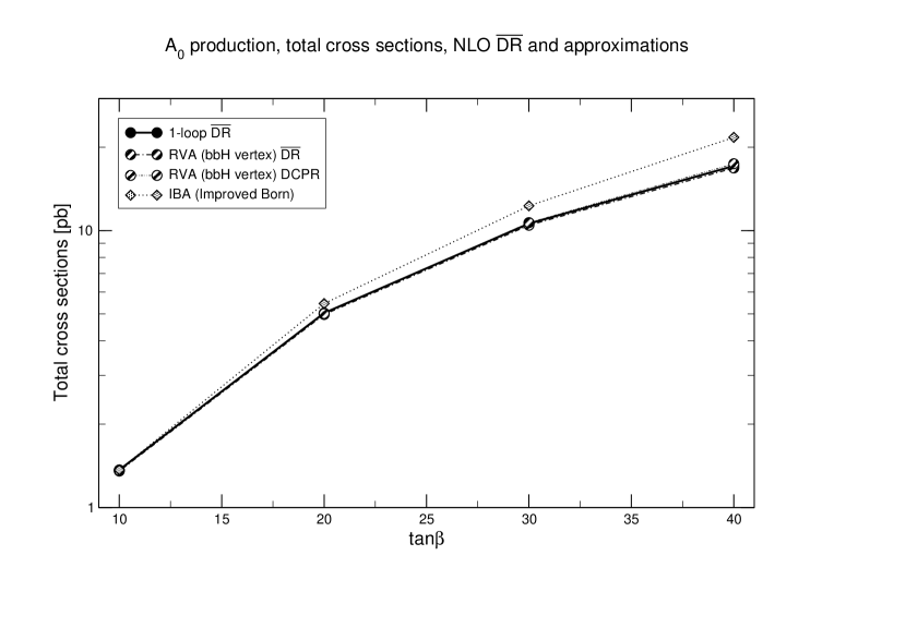
Figure 11: Comparison of the total NLO cross sections: NLO $\overline{\rm DR}$ , RVA ($\overline{\rm DR}$ and DCPR) and Improved Born Approximantion (IBA), $A^{0}$ production; $M_{A^{0}}=250$ GeV, $p_{b,T}>20$ GeV, $|y_{b}|<2$.

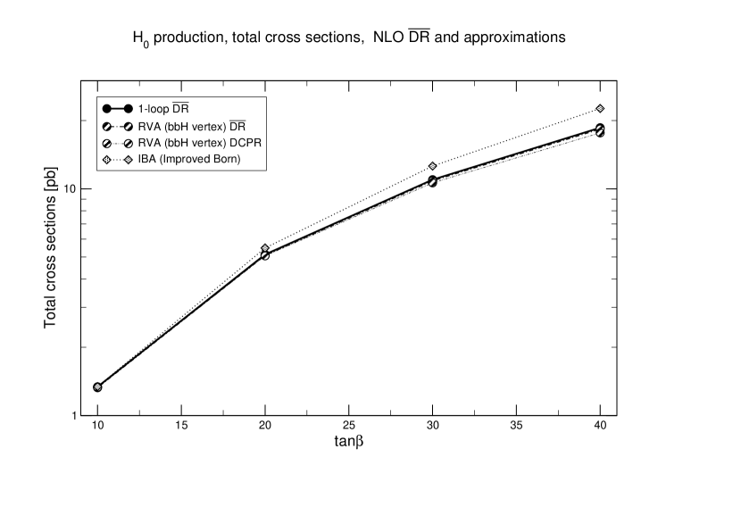
Figure 12: Comparison of the total NLO cross sections: NLO $\overline{\rm DR}$ , RVA ($\overline{\rm DR}$ and DCPR) and Improved Born Approximantion (IBA), $H^{0}$ production; $M_{A^{0}}=250$ GeV, $p_{b,T}>20$ GeV, $|y_{b}|<2$.

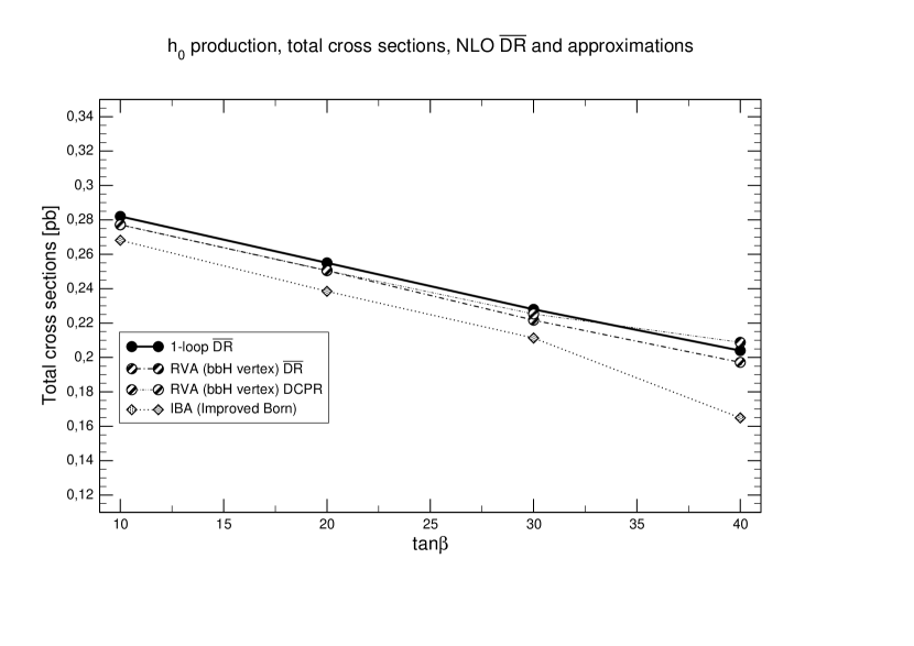
Figure 13: Comparison of the total NLO cross sections: NLO $\overline{\rm DR}$ , RVA ($\overline{\rm DR}$ and DCPR) and Improved Born Approximantion (IBA), $h^{0}$ production; $M_{A^{0}}=250$ GeV, $p_{b,T}>20$ GeV, $|y_{b}|<2$.

As one can see from the plots, (Figures 11,12,13) this version of IBA is sufficiently close to the complete calculation only for relatively small $\tan\beta$ values, roughly $\tan\beta<20$. In this range, the approximation gives larger (compared to the complete calculation) rates for $H^{0},\,A^{0}$ and smaller rates for $h^{0}$. The differences remain below the ten percent size, which would be tolerable at least in a first phase of LHC measurements. Increasing the $\tan\beta$ value, the IBA description becomes worse. For $\tan\beta=40$, it differs in all the three cases by, roughly, a relative 25 percent, which seems a rather poor prediction for the measurable total rates.

For what concerns the $\tan\beta$ dependence of the plots, one can conclude that it provides those features that would be expected at the chosen value of $M_{A^{0}}$, which is sufficiently larger than $M_{Z}$ to approach the correct “decoupling” limits. In this large $M_{A^{0}}$ regime, that is discussed widely in the literature (see e.g. Djouadi:2005gj ), the $H^{0}$ and $A^{0}$ couplings become almost exactly proportional to $\tan\beta$, while the $h^{0}$ coupling becomes very weakly $\tan\beta$ dependent. These features are well reproduced by the plots, that show a roughly quadratic $\tan\beta$ dependence of the $H^{0},\;A^{0}$ rates and a much weaker $\tan\beta$ dependence for $h^{0}$. But for large $\tan\beta$ values, there seems to be an extra $\tan\beta$ dependence of the complete calculation that is not contained in the IBA description.

Having this apparent discrepancy in our mind, as a second attempt, we have tried to use what we would call a “Reduced Vertex Approximation” (RVA): we approximate the complete NLO keeping only the (all) one loop corrections to the “final” Yukawa $bb\mathcal{H}^{0}$ vertex and the subset of counterterms needed to get a UV-finite result; the photon mass is regulated (arbitrarily) as $M_{\gamma}=M_{Z}$ (and thus we do not include soft and hard radiation). We kept the one loop Higgs masses in the kinematics as well as the $Z$-factors in the definition of the cross section; all the other diagrams (Boxes, Initial and Up Triangles, Self Energies) are neglected. As a check we computed the cross section in this approximation in both schemes (the subset of diagrams, with the right choice of counterterms, should be scheme independent). As one can see from the updated figures our RVA turns out to provide very efficient description of the total NLO cross sections; the difference between the NLO and the RVA is of order of $1\%$, $3.4\%$ in the worst case. This is numerically summarized in Tables 6,7,8 and Figures 11,12,13.

From the inspection of those Tables and Figures we would conclude that the extra vertices that the RVA contains seem to provide the extra $\tan\beta$ dependence not predicted by the IBA in a reasonably satisfactory way, i.e. at the level of few percent in the full $\tan\beta$ range. This RVA cannot be transformed into simple analytical expressions. It tells us that the relative effect of a large set of Feynman diagrams, those that were not included in the approximation, is small, at the level of a few percent, which might be considered negligible for the first phase of LHC measurements.

$\tan\beta$	$\;\sigma^{\mbox{\tiny{$\overline{\rm DR}$~{},NLO}}}\;$	RVAbbH	$\sigma/$RVAbbH	IBA	$\sigma/$IBA
10	1.338	1.32623	1.00888	1.34087	0.997861
20	5.133	5.08324	1.00979	5.48397	0.936
30	10.975	10.8433	1.01215	12.6044	0.87073
40	18.613	18.3461	1.01455	22.6229	0.822749

Table 6: $H^{0}$ production: comparison between the complete NLO prediction and the two approximations: total cross sections and ratios $\;\sigma^{\mbox{\tiny{$\overline{\rm DR}$~{},NLO}}}/\sigma_{\textrm{\tiny{APP.}}}$.

$\tan\beta$	$\;\sigma^{\mbox{\tiny{$\overline{\rm DR}$~{},NLO}}}\;$	RVAbbH	$\sigma/$RVAbbH	IBA	$\sigma/$IBA
10	0.282	0.277157	1.01747	0.268161	1.05161
20	0.255	0.250495	1.01799	0.238459	1.06936
30	0.228	0.221673	1.02854	0.211275	1.07916
40	0.204	0.197159	1.0347	0.164874	1.23731

Table 7: $h^{0}$ production: comparison between the complete NLO prediction and the two approximations: total cross sections and ratios $\;\sigma^{\mbox{\tiny{$\overline{\rm DR}$~{},NLO}}}/\sigma_{\textrm{\tiny{APP.}}}$.

$\tan\beta$	$\;\sigma^{\mbox{\tiny{$\overline{\rm DR}$~{},NLO}}}\;$	RVAbbH	$\sigma/$RVAbbH	IBA	$\sigma/$IBA
10	1.367	1.35328	1.01014	1.36737	0.999729
20	5.04	4.98026	1.01199	5.4543	0.924042
30	10.601	10.4581	1.01366	12.2948	0.862232
40	17.118	16.8292	1.01716	21.7326	0.787663

Table 8: $A^{0}$ production: comparison between the complete NLO prediction and the two approximations: total cross sections and ratios $\;\sigma^{\mbox{\tiny{$\overline{\rm DR}$~{},NLO}}}/\sigma_{\textrm{\tiny{APP.}}}$.

V Conclusions

We have performed in this paper a complete MSSM calculation of the electroweak NLO effect in the processes of semi-inclusive bottom-Higgs production. Our analysis has been performed for two choices of the $M_{A^{0}}$ input parameter and for variable values of the $\tan\beta$ parameter defined in the $\overline{\rm DR}$ renormalization scheme. Although a more extended analysis of the parameter space would be interesting, we have found certain results that appear to us to be general and worth publishing. The first conclusion is that two different renormalization schemes appear to be practically identical at SUSY NLO as one would a priori expect. Working in the $\overline{\rm DR}$ scheme, that seemed to us to be somehow preferable, we have found that the pure electroweak one-loop effect in the three considered production processes is of a size that might be relevant and therefore that this contribution cannot be ignored for a proper experimental analysis of the reactions.

There could exist simpler calculations involving a smaller (but still large) number of diagrams, that would provide a valid numerical result. We have seen that one possible Improved Born Approximation does not reproduce the correct result in a satisfactory way. We have also seen that another “Reduced Vertex Approximation” (which considers only the 1-loop correction to the Yukawa $bb\mathcal{H}^{0}$ vertex) appears to better approximate the full NLO.

However, if a theoretical prediction of the total cross section is requested at the percent level, which might be the hopefully desirable final LHC goal, our conclusion is that the complete one-loop calculation of the electroweak part that we have performed in this paper should be considered, together with the available, large, QCD corrections, as the correct proposal to offer to the experimental community.

There remains a couple of relevant points to be still investigated. The first is that of combining this analysis with an analogous one to be performed for the process of associated top-charged Higgs production, for which our group has already provided a complete one-loop electroweak analysis Beccaria:2009my . The second one is that of trying to relate the $\overline{\rm DR}$ $\tan\beta$ parameter, which is not a measurable quantity, to a measurable $\tan\beta$ (which could be defined for instance by $A^{0}\to\tau^{+}\tau^{-}$ decay as suggested in schemes ). This would allow to draw plots where also the horizontal axis represents a measurable quantity. These points are, in our opinion, quite relevant but beyond the purposes of our analysis; work is in progress on these issues.

Appendix A Renormalization constants in the Higgs sector

The renormalization constants of the wavefunction of the Higgs bosons $A^{0},h^{0},H^{0}$ and of the Goldstone boson $G^{0}$ are given by

$$\delta\bar{Z}_{H^{0}H^{0}}=\cos^{2}\alpha\delta Z_{H1}+\sin^{2}\alpha\delta Z_{H2},~{}~{}~{}\delta\bar{Z}_{H^{0}h^{0}}=\sin\alpha\cos\alpha(\delta Z_{H2}-\delta Z_{H1}),$$

$$\delta\bar{Z}_{h^{0}h^{0}}=\sin^{2}\alpha\delta Z_{H1}+\cos^{2}\alpha\delta Z_{H2},~{}~{}~{}~{}\delta\bar{Z}_{A^{0}A^{0}}=\sin^{2}\beta\delta Z_{H1}+\cos^{2}\beta\delta Z_{H2},$$

$$\delta\bar{Z}_{G^{0}A^{0}}=\cos\beta\sin\beta(\delta Z_{H2}-\delta Z_{H1}),~{}~{}~{}\delta\bar{Z}_{h^{0}A^{0}}=\delta\bar{Z}_{H^{0}A^{0}}=\delta\bar{Z}_{h^{0}G^{0}}=\delta\bar{Z}_{H^{0}G^{0}}=0.$$

The renormalization constants for the $c^{\eta}(bbh^{0})$ and for the $c^{\eta}(bbH^{0})$ couplings is obtained differentiating the tree-level expressions in Eq. (5),

$$\delta c^{\eta}(bbh^{0}) = \left({\delta g\over g}+{\delta m_{b}\over m_{b}}-{\delta M^{2}_{W}\over 2M^{2}_{W}}-{\delta\cos\beta\over\cos\beta}\right)c^{\eta}(bbh^{0}),$$

$$\delta c^{\eta}(bbH^{0}) = \left({\delta g\over g}+{\delta m_{b}\over m_{b}}-{\delta M^{2}_{W}\over 2M^{2}_{W}}-{\delta\cos\beta\over\cos\beta}\right)c^{\eta}(bbH^{0}).$$ (31)

$\delta\cos\beta$, $\delta M^{2}_{W}$, and $\delta g$, reads as follows

$$\delta\cos\beta = -\sin^{2}\beta{\delta\tan\beta\over\tan\beta},$$

$$\delta M^{2}_{W} = \mbox{Re}\Sigma_{W}(M^{2}_{W}),$$

$${\delta g\over g} = {\Sigma_{\gamma Z}(0)\over s_{W}c_{W}M^{2}_{Z}}-\frac{1}{2}\Bigg{[}+2{c_{W}\over s_{W}M^{2}_{Z}}\Sigma_{\gamma Z}(0)+{c^{2}_{W}\over s^{2}_{W}}\left({\delta M^{2}_{Z}\over M^{2}_{Z}}-{\delta M^{2}_{W}\over M^{2}_{W}}\right)-\Sigma^{\prime}_{\gamma\gamma}(0)\Bigg{]},$$ (32)

with $\delta M^{2}_{Z}=\mbox{Re}\Sigma_{Z}(M^{2}_{Z})$. The $c^{\eta}(bbA^{0})$ couplings depends only on the angle $\beta$. When computing the the renormalization constant $\delta c^{\eta}(bbA^{0})$, one has to distinguish between the $\beta$-dependent factors originated by the $H_{1}$, $H_{2}$ mixing and the $\beta$- dependent factors from the $H_{1}$, $H_{2}$ couplings. Only the latter have to be renormalized. In particular the factor $\sin\beta$ [$1/\cos\beta$] entering the $c^{\eta}(bbA^{0})$ coupling is originated from the $H_{1}$, $H_{2}$ mixing [couplings], and thus $\delta c^{\eta}(bbA^{0})$ reads

$$\delta c^{\eta}(bbA^{0})=\left({\delta g\over g}+{\delta m_{b}\over m_{b}}-{\delta M^{2}_{W}\over 2M^{2}_{W}}-{\delta\cos\beta\over\cos\beta}\right)c^{\eta}(bbA^{0}).$$ (33)

Appendix B Contributions of the counterterms

In this appendix we list explicitely the contributions of the counterterms writen in terms of the renormalization constants introduced in Section II.3 and in Appendix A. The vertices counterterms can be written as follows

$$\bar{u}^{\prime}_{b}(\lambda^{\prime}_{b})\left(\sum_{k=1}^{4}\sum_{\eta=L,R}J^{k\eta}V^{k\eta}_{bg\to b\mathcal{H}^{0}}\right)u_{b}(\lambda_{b}),$$ (34)

where $J^{k\eta}$ are defined in Eq. (8) while the non-zero $V^{k\eta}_{bg\to b\mathcal{H}^{0}}$ reads

$$V^{1\eta}_{bg\to b\mathcal{H}^{0}} = {g_{s}\over s-m^{2}_{b}}\left\{\left({3\over 2}\delta Z^{b}_{\eta}+{1\over 2}\delta Z^{b}_{\bar{\eta}}\right)c^{\eta}(bb\mathcal{H}^{0})+\delta c^{\eta}(bb\mathcal{H}^{0})+{1\over 2}\sum_{\bar{\mathcal{H}}^{0}}\delta\bar{Z}^{*}_{\bar{\mathcal{H}}^{0}\mathcal{H}^{0}}c^{\eta}(bb\bar{\mathcal{H}}^{0})\right\}$$

$$- {g_{s}\over u-m^{2}_{b}}\left\{\left({3\over 2}\delta Z^{b}_{\bar{\eta}}+{1\over 2}\delta Z^{b}_{\eta}\right)c^{\eta}(bb\mathcal{H}^{0})+\delta c^{\eta}(bb\mathcal{H}^{0})+{1\over 2}\sum_{\bar{\mathcal{H}}^{0}}\delta\bar{Z}^{*}_{\bar{\mathcal{H}}^{0}\mathcal{H}^{0}}c^{\eta}(bb\bar{\mathcal{H}}^{0})\right\},$$

$$V^{2\eta}_{bg\to b\mathcal{H}^{0}} = {-2g_{s}\over u-m^{2}_{b}}\left\{\left({3\over 2}\delta Z^{b}_{\bar{\eta}}+{1\over 2}\delta Z^{b}_{\eta}\right)c^{\eta}(bb\mathcal{H}^{0})+\delta c^{\eta}(bb\mathcal{H}^{0})+{1\over 2}\sum_{\bar{\mathcal{H}}^{0}}\delta\bar{Z}^{*}_{\bar{\mathcal{H}}^{0}\mathcal{H}^{0}}c^{\eta}(bb\bar{\mathcal{H}}^{0})\right\},$$

$$V^{3\eta}_{bg\to b\mathcal{H}^{0}} = {m_{b}g_{s}\over s-m^{2}_{b}}\left(\delta Z^{b}_{\bar{\eta}}-\delta Z^{b}_{\eta}\right)c^{\bar{\eta}}(bb\mathcal{H}^{0})+{m_{b}g_{s}\over u-m^{2}_{b}}\left(\delta Z^{b}_{\bar{\eta}}-\delta Z^{b}_{\eta}\right)c^{\eta}(bb\mathcal{H}^{0}),$$ (35)

where $(\eta,\bar{\eta})\in\{(L,R);\,(R,L)\}$ and $\mathcal{H}^{0},\bar{\mathcal{H}}^{0}=h^{0},H^{0},A^{0},G^{0}$. The bottom self energy counterterm reads as follows

$$\bar{u}^{\prime}_{b}(\lambda^{\prime}_{b})\left(\sum_{k=1}^{4}\sum_{\eta=L,R}J^{k\eta}S^{k\eta}_{bg\to b\mathcal{H}^{0}}\right)u_{b}(\lambda_{b}).$$ (36)

The non-zero $S^{k\eta}_{bg\to b\mathcal{H}^{0}}$ are

$$S^{1\eta}_{bg\to b\mathcal{H}^{0}} = g_{s}{c^{\eta}(bb\mathcal{H}^{0})\over(s-m^{2}_{b})^{2}}\left\{s\delta Z^{b}_{\eta}-m^{2}_{b}\left(\delta Z^{b}_{\eta}-2{\delta m_{b}\over m_{b}}\right)\right\}$$

$$+ g_{s}{c^{\eta}(bb\mathcal{H}^{0})\over(u-m^{2}_{b})^{2}}\left\{u\delta Z^{b}_{\bar{\eta}}-m^{2}_{b}\left(\delta Z^{b}_{\bar{\eta}}-2{\delta m_{b}\over m_{b}}\right)\right\}$$

$$S^{2\eta}_{bg\to b\mathcal{H}^{0}} = 2g_{s}{c^{\eta}(bb\mathcal{H}^{0})\over(u-m^{2}_{b})^{2}}\left\{u\delta Z^{b}_{\bar{\eta}}-m^{2}_{b}\left(\delta Z^{b}_{\bar{\eta}}-2{\delta m_{b}\over m_{b}}\right)\right\}$$

$$S^{3\eta}_{bg\to b\mathcal{H}^{0}} = g_{s}m_{b}{c^{\bar{\eta}}(bb\mathcal{H}^{0})\over(s-m^{2}_{b})}\left\{{1\over 2}\left(\delta Z^{b}_{\eta}-\delta Z^{b}_{\bar{\eta}}\right)-~{}{\delta m_{b}\over m_{b}}\right\}$$ (37)

$$+ g_{s}m_{b}{c^{\eta}(bb\mathcal{H}^{0})\over(u-m^{2}_{b})}\left\{{1\over 2}\left(\delta Z^{b}_{\eta}-\delta Z^{b}_{\bar{\eta}}\right)-{\delta m_{b}\over m_{b}}\right\}$$

Figure 1: Tree level diagrams for the partonic $bg\to b\mathcal{H}^{0}$ processes.

Figure 2: Bottom quark self energies, higgs self energies (only the diagonal case) and internal self energies.

Figure 3: Triangle and box diagrams.

Figure 4: Real photon $\gamma$ emission.

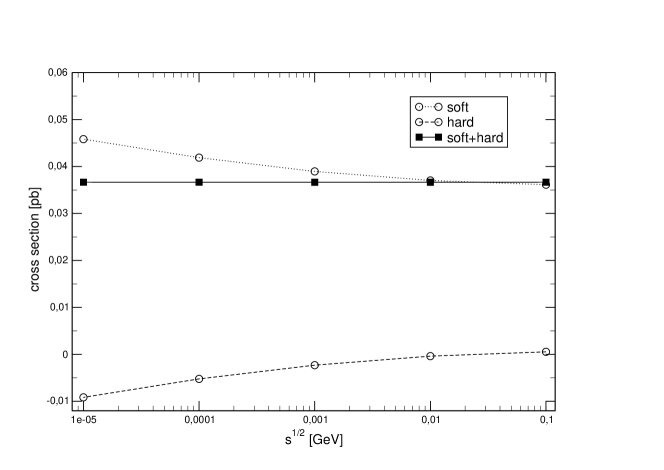
Figure 6: $H^{0}$ production: dependence of the $\mathcal{O}(\alpha)$ soft+virtual, hard, and total sum corrections on the separator $\Delta E$

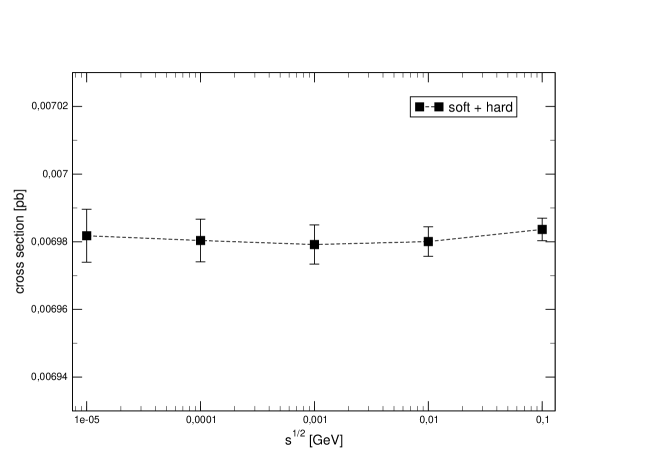
Figure 7: $h^{0}$ production: dependence of the $\mathcal{O}(\alpha)$ soft+virtual, hard, and total sum corrections on the separator $\Delta E$

Figure 9: Total LO and NLO cross sections in the $\overline{\rm DR}$ and DCPR schemes, $H^{0}$ production; $M_{A^{0}}=250$ GeV, $p_{b,T}>20$ GeV, $|y_{b}|<2$.

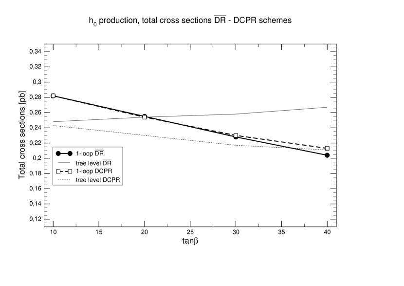
Figure 10: Total LO and NLO cross sections in the $\overline{\rm DR}$ and DCPR schemes, $h^{0}$ production; $M_{A^{0}}=250$ GeV, $p_{b,T}>20$ GeV, $|y_{b}|<2$.

Figure 16: Invariant mass distribution, $H^{0}$ production, $\overline{\rm DR}$ scheme. $M_{A^{0}}=250$ GeV, $\tan\beta=30$ $p_{b,T}>20$ GeV, $|y_{b}|<2$.

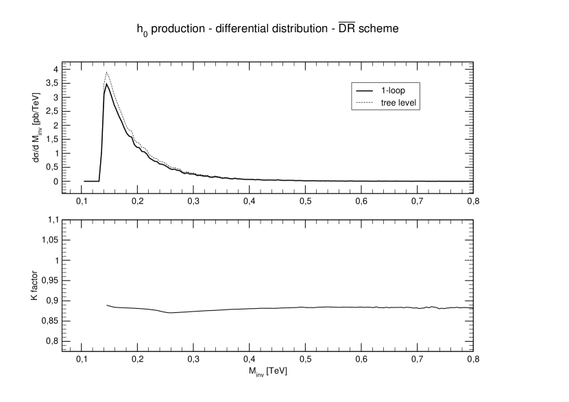
Figure 17: Invariant mass distribution, $h^{0}$ production, $\overline{\rm DR}$ scheme. $M_{A^{0}}=250$ GeV, $\tan\beta=30$ $p_{b,T}>20$ GeV, $|y_{b}|<2$.

Figure 18: Invariant mass distribution, $A^{0}$ production, $\overline{\rm DR}$ scheme. $M_{A^{0}}=350$ GeV, $\tan\beta=15$ $p_{b,T}>20$ GeV, $|y_{b}|<2$.

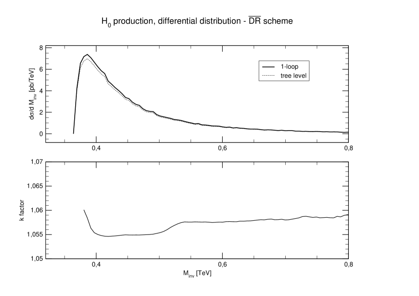
Figure 19: Invariant mass distribution, $H^{0}$ production, $\overline{\rm DR}$ scheme. $M_{A^{0}}=350$ GeV, $\tan\beta=15$ $p_{b,T}>20$ GeV, $|y_{b}|<2$.

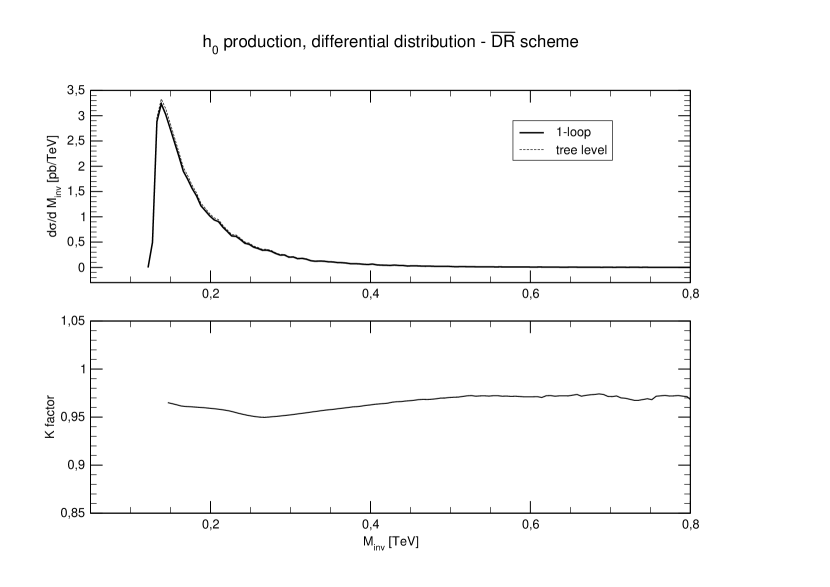
Figure 20: Invariant mass distribution, $h^{0}$ production, $\overline{\rm DR}$ scheme. $M_{A^{0}}=350$ GeV, $\tan\beta=15$ $p_{b,T}>20$ GeV, $|y_{b}|<2$.

References

- (1) J. M. Campbell et al., Higgs boson production in association with bottom quarks arXiv:hep-ph/0405302.
- (2) D. Dicus, T. Stelzer, Z. Sullivan and S. Willenbrock, Higgs boson production in association with bottom quarks at next-to-leading order, Phys. Rev. D 59, 094016 (1999) [arXiv:hep-ph/9811492].
- (3) J. M. Campbell, R. K. Ellis, F. Maltoni and S. Willenbrock, Higgs boson production in association with a single bottom quark Phys. Rev. D 67 (2003) 095002 [arXiv:hep-ph/0204093].
- (4) R. V. Harlander and W. B. Kilgore, Higgs boson production in bottom quark fusion at next-to-next-to-leading order, Phys. Rev. D 68, 013001 (2003) [arXiv:hep-ph/0304035].
- (5) S. Dittmaier, M. Kramer, A. Muck and T. Schluter, MSSM Higgs-boson production in bottom-quark fusion: Electroweak radiative corrections, JHEP 0703, 114 (2007) [arXiv:hep-ph/0611353].
- (6) S. Dawson, C. B. Jackson, L. Reina, and D. Wackeroth. Higgs boson production with one bottom quark jet at hadron colliders,Phys. Rev. Lett., 94:031802, 2005.
- (7) S. Dawson and C. B. Jackson, SUSY QCD Corrections to Associated Higgs-bottom Quark Production, Phys. Rev. D 77, 015019 (2008) [arXiv:0709.4519 [hep-ph]].
- (8) S. Dawson and P. Jaiswal, Weak Corrections to Associated Higgs-Bottom Quark Production, [arXiv:hep-ph/1002.2672].
- (9) S. Dawson, C. B. Jackson, L. Reina and D. Wackeroth, Higgs production in association with bottom quarks at hadron colliders, Mod. Phys. Lett. A 21, 89 (2006) [arXiv:hep-ph/0508293].
- (10) Stefan Dittmaier, Michael Kramer, and Michael Spira. Higgs radiation off bottom quarks at the tevatron and the LHC,Phys. Rev., D70:074010, 2004.
- (11) S. Dawson, C. B. Jackson, L. Reina and D. Wackeroth, Phys. Rev. D 69 (2004) 074027 [arXiv:hep-ph/0311067].
- (12) F. Boudjema and L. D. Ninh, Leading Yukawa corrections to Higgs production associated with a tagged bottom anti-bottom pair in the Standard Model at the LHC, Phys. Rev. D 77, 033003 (2008) [arXiv:0711.2005 [hep-ph]].
- (13) G. Gao, R. J. Oakes and J. M. Yang, Heavy supersymmetric particle effects in Higgs boson production associated with a bottom quark pair at LHC, Phys. Rev. D 71, 095005 (2005) [arXiv:hep-ph/0412356].
- (14) M. Frank, T. Hahn, S. Heinemeyer, W. Hollik, H. Rzehak and G. Weiglein, The Higgs boson masses and mixings of the complex MSSM in the Feynman-diagrammatic approach JHEP 0702 (2007) 047 [arXiv:hep-ph/0611326].
- (15) A. Dabelstein, The One loop renormalization of the MSSM Higgs sector and its application to the neutral scalar Higgs masses Z. Phys. C 67 (1995) 495 [arXiv:hep-ph/9409375].
- (16) P. H. Chankowski, S. Pokorski and J. Rosiek, Complete on-shell renormalization scheme for the minimal supersymmetric Higgs sector Nucl. Phys. B 423 (1994) 437 [arXiv:hep-ph/9303309].
- (17) S. Heinemeyer, W. Hollik, H. Rzehak and G. Weiglein, High-precision predictions for the MSSM Higgs sector at O(alpha(b) alpha(s)) Eur. Phys. J. C 39 (2005) 465 [arXiv:hep-ph/0411114].
-
(18)
J. Kublbeck, M. Bohm and A. Denner,
FeynArts: Computer algebraic generation of Feynman graphs and amplitudes
Comput. Phys. Commun. 60, 165 (1990).
T. Hahn, Generating Feynman diagrams and amplitudes with FeynArts 3 Comput. Phys. Commun. 140, 418 (2001) [arXiv:hep-ph/0012260].
T. Hahn and C. Schappacher, The implementation of the minimal supersymmetric standard model in FeynArts and FormCalc Comput. Phys. Commun. 143, 54 (2002) [arXiv:hep-ph/0105349]. -
(19)
T. Hahn and M. Perez-Victoria,
Automatized one-loop calculations in four and D dimensions
Comput. Phys. Commun. 118, 153 (1999)
[arXiv:hep-ph/9807565].
T. Hahn and M. Rauch, News from FormCalc and LoopTools Nucl. Phys. Proc. Suppl. 157, 236 (2006) [arXiv:hep-ph/0601248]. - (20) V. N. Baier, V. S. Fadin and V. A. Khoze, Quasireal electron method in high-energy quantum electrodynamics, Nucl. Phys. B 65, 381 (1973).
- (21) U. Baur, S. Keller and D. Wackeroth, Electroweak radiative corrections to boson production in hadronic collisions Phys. Rev. D 59, 013002 (1999) [arXiv:hep-ph/9807417].
- (22) S. Dittmaier, A general approach to photon radiation off fermions Nucl. Phys. B 565, 69 (2000) [arXiv:hep-ph/9904440].
- (23) S. Heinemeyer, W. Hollik and G. Weiglein, FeynHiggs: a program for the calculation of the masses of the neutral CP-even Higgs bosons in the MSSM Comput. Phys. Commun. 124 (2000) 76 [arXiv:hep-ph/9812320].
- (24) J. H. Kuhn, A. Kulesza, S. Pozzorini and M. Schulze, Electroweak corrections to hadronic production of W bosons at large transverse momenta Nucl. Phys. B 797, 27 (2008) [arXiv:0708.0476 [hep-ph]].
- (25) M. Beccaria, G. Macorini, E. Mirabella, L. Panizzi, F. M. Renard and C. Verzegnassi, One-loop electroweak effects on stop-chargino production at LHC [arXiv:0812.4375 [hep-ph]].
- (26) M. Beccaria, G. Macorini, L. Panizzi, F. M. Renard and C. Verzegnassi, Associated production of charged Higgs and top at LHC: the role of the complete electroweak supersymmetric contribution Phys. Rev. D 80 (2009) 053011 [arXiv:0908.1332 [hep-ph]].
- (27) J. Pumplin, D. R. Stump, J. Huston, H. L. Lai, P. M. Nadolsky and W. K. Tung, New generation of parton distributions with uncertainties from global QCD analysis JHEP 0207 (2002) 012 [arXiv:hep-ph/0201195].
- (28) M. Roth and S. Weinzierl, QED corrections to the evolution of parton distributions Phys. Lett. B 590, 190 (2004)
- (29) See A. Freitas and D. Stockinger, Gauge dependence and renormalization of in the MSSM Phys. Rev. D 66, 095014 (2002) [arXiv:hep-ph/0205281], and references therein.
- (30) A. Djouadi, Phys. Rept. 459 (2008) 1 [arXiv:hep-ph/0503173].