Characterising Complexity in Solar Magnetogram Data using a Wavelet-based Segmentation Method

Abstract

The multifractal nature of solar photospheric magnetic structures are studied using the 2D wavelet transform modulus maxima (WTMM) method. This relies on computing partition functions from the wavelet transform skeleton defined by the WTMM method. This skeleton provides an adaptive space-scale partition of the fractal distribution under study, from which one can extract the multifractal singularity spectrum. We describe the implementation of a multiscale image processing segmentation procedure based on the partitioning of the WT skeleton which allows the disentangling of the information concerning the multifractal properties of active regions from the surrounding quiet-Sun field. The quiet Sun exhibits a average Hölder exponent $\sim-0.75$, with observed multifractal properties due to the supergranular structure. On the other hand, active region multifractal spectra exhibit an average Hölder exponent $\sim 0.38$ similar to those found when studying experimental data from turbulent flows.

1 Introduction

Since the late 70’s and the propagation of fractal ideas throughout the scientific community (Mandelbrot, 1982), there have been numerous applications of the concepts of scale invariance, self-similarity, long-range dependence in many areas of physics, chemistry, biology, geology, meteorology, economy, social and material sciences (Aharony & Feder, 1989; West, 1990; Vicsek et al., 1994; Bunde & Havlin, 1994; Wilkinson et al., 1995; Family et al., 1995; Frisch, 1995; Arneodo et al., 1995a; Bunde et al., 2002). Various methods were developed to quantify scale-invariance properties through the computation of the fractal dimension $D_{F}$ for self-similar objects or the roughness exponent $H$ for self-affine fractals (Mandelbrot, 1982; Peitgen & Saupe, 1987; Feder, 1988; Argoul et al., 1990; Lea-Cox & Wang, 1993; Wilkinson et al., 1995; Taqqu et al., 1995). Unfortunately $D_{F}$ and $H$ are global quantities that do not account for the possibility of point-to-point fluctuations of the scaling properties of a fractal object. The multifractal formalism was introduced in the mid-eighties to provide a statistical description of the fluctuations of regularity of singular measures that are found in chaotic dynamical systems (Halsey et al., 1986; Collet et al., 1987; Rand, 1989) or in modelling of the energy cascading process in turbulent flows (Mandelbrot, 1974; Paladin & Vulpiani, 1987; Mandelbrot, 1989; Meneveau & Sreenivasan, 1991). Box-counting and correlation algorithms were successfully adapted to resolve multifractal scaling for isotropic self-similar fractals by computation of the generalized fractal dimensions $D_{q}$ (Grassberger & Procaccia, 1983a, b; Grassberger et al., 1988). As to self-affine fractals, Parisi and Frisch (Parisi & Frisch, 1985) proposed, for the analysis of fully-developed turbulence velocity data, an alternative multifractal description based on the investigation of the scaling behavior of the so-called structure functions (Frisch, 1995; Monin & Yaglom, 1975): $S_{p}(l)=<(\delta v_{l})^{p}>\sim l^{\zeta_{p}}$ ($p$ integer $>0$), where $\delta v_{l}(x)=v(x+l)-v(x)\sim l^{h(x)}$ is an increment of the recorded signal over a distance $l$. Then, after reinterpreting the roughness exponent as a local quantity (Parisi & Frisch, 1985; Muzy et al., 1991, 1994; Arneodo et al., 1995c): $\delta v_{l}(x)\sim l^{h(x)}$ (power-law behavior), the $D(h)$ singularity spectrum is defined as the Hausdorff dimension of the set of points $x$ where the local roughness (or Hölder) exponent $h(x)$ of $v$ is $h$. In principle, $D(h)$ can be attained by Legendre transforming the structure function scaling exponents $\zeta_{p}$ (Parisi & Frisch, 1985; Muzy et al., 1991, 1994; Arneodo et al., 1995c). Unfortunately, as noticed by (Muzy et al., 1991, 1993, 1994), both the box-counting and structure function methodology have intrinsic limitations and fail to fully characterize the corresponding singularity spectrum since only the strongest singularities are a priori amenable to these techniques. As such, both methods are limited in their application to real data sets (Muzy et al., 1994; Georgoulis, 2005; Conlon et al., 2008).

In previous work, Arneodo and collaborators (Muzy et al., 1991, 1993, 1994; Arneodo et al., 1995c) have shown that there exists a natural way of performing a unified multifractal analysis of both singular measures and multi-affine functions, which consists in using the continuous wavelet transform (Goupillaud et al., 1984; Grossmann & Morlet, 1984; Meyer, 1990; Daubechies, 1992; Mallat, 1998). By using wavelets instead of boxes, one can take advantage of the freedom of the choice of these “generalized oscillating boxes” to get rid of possible smooth behavior that might either mask singularities or perturb the estimation of their strength $h$. The other fundamental advantage of using wavelets is that the skeleton defined by the wavelet transform modulus maxima (WTMM) (Mallat & Zhong, 1992; Mallat & Hwang, 1992), provides an adaptative space-scale partitioning from which one can extract the $D(h)$ singularity spectrum via the scaling exponent $\tau(q)$ of some partition functions defined from the WT skeleton. The so-called WTMM method (Muzy et al., 1991, 1993, 1994; Arneodo et al., 1995c) therefore gives access to the entire $D(h)$ spectrum via the usual Legendre transform $D(h)=min_{q}(qh-\tau(q))$. We refer the reader to Bacry et al. (1993) and Jaffard (1997) for rigorous mathematical results and to Hentschel (1994) for the theoretical treatment of random multifractal functions.

Applications of the WTMM method to 1D signals have already provided insight into a wide variety of problems (Arneodo et al., 2002), e.g. the validation of the log-normal cascade phenomenology of fully developed turbulence (Arneodo et al., 1998a, 1999b; Delour et al., 2001) and of high-resolution temporal rainfall (Venugopal et al., 2006a, b; Roux et al., 2009), the characterization and the understanding of long-range correlations in DNA sequences (Arneodo et al., 1995b, 1996; Audit et al., 2001, 2002), the demonstration of the existence of a causal cascade of information from large to small scales in financial time series (Arneodo et al., 1998b; Muzy et al., 2000), the use of the multifractal formalism to discriminate between healthy and sick heartbeat dynamics (Ivanov et al., 1996, 1999), the discovery of a Fibonacci structural ordering in 1D cuts of diffusion limited aggregates (Arneodo et al., 1992a, b, c; Kuhn et al., 1994) and in hard X-ray emission from solar flares (McAteer et al., 2007). The WTMM method has been generalized from 1D to 2D with the specific goal to achieve multifractal analysis of rough surfaces  with fractal dimension $D_{F}$ anywhere between 2 and 3 (Arrault et al., 1997; Arneodo et al., 2000; Decoster et al., 2000). The 2D WTMM method has been successfully applied to characterize the intermittent nature of cloud structure from satellite images (Arneodo et al., 1999a; Roux et al., 2000) and to assist in the diagnosis of breast tissue lesions in digitized mammograms (Kestener et al., 2001). In astrophysics, this method was adapted and used to characterize the anisotropic structure of atomic hydrogen gas (HI) in the Galatic disk (Khalil et al., 2006). From the analysis of very large mosaics taken from the Canadian Galatic Plane Survey (Taylor et al., 2003), directional roughness exponents were introduced to show that the HI in the Galactic spiral arms has a scale-dependent anisotropic signature while the HI in the inter-spiral arm regions exhibits scale-independent anisotropy. Along that line, the 2D WTMM method was further applied to characterize the space-scale nature of anisotropic structures (Snow et al., 2008a, b; Khalil et al., 2009) and to perform objective segmentation of image features of interest from noisy backgrounds (Khalil et al., 2007; Caddle et al., 2007; Roland et al., 2009). We refer the reader to Arneodo et al. (2003) for a review of the 2D WTMM methodology, from the theoretical concepts to experimental applications. Recently, the WTMM method has been further extended to 3D scalar (Kestener & Arneodo, 2003) as well as 3D vector (Kestener & Arneodo, 2004, 2007) fields analysis and applied to 3D (velocity, vorticity, dissipation, enstrophy) numerical data issued from direct numerical simulations (DNS) of incompressible Navier-Stokes equations. Because it combines singular-value decomposition and multifractal description, the so-called tensorial wavelet transform modulus maxima method for vector fields (Kestener & Arneodo, 2004, 2007) looks very promising for future simultaneous multifractal and structural (vorticity sheets, vorticity filaments) analysis of turbulent flows.

Our aim here is to exploit the ability of the WTMM method to study compound systems that display some non-analyticity in their multifractal spectra as the signature of some phase transition between two underlying scale invariant components with different multifractal properties (Bohr & Tèl, 1988; Muzy et al., 1994; Arneodo et al., 1995c). These two components can both have some physical significance as previously experienced when using the WTMM method to detect vorticity filaments in swirling turbulent flows (Roux et al., 1999) or microcalcifications from breast tissue background in digitized mammograms (Kestener et al., 2001; Arneodo et al., 2003). One of these components can be noise that may cause drastic distortions in the returned multifractal spectra. In this work we will follow a wavelet-based strategy inspired from the one previously used in 1D to detect replication origins and promoters as jumps (discontinuities) in 1D noisy skew profiles in mammalian genomes (Brodie of Brodie et al., 2005; Touchon et al., 2005; Nicolay et al., 2007) and in 2D to perform an objective and automatic segmentation of chromosome territories in fluorescence microscopy imaging of mouse cell nuclei (Khalil et al., 2007; Caddle et al., 2007) and of gold formation on vapodeposited thin gold films (Roland et al., 2009).

The purpose of the manuscript is to demonstrate the suitability and reliability of the WTMM method to propose a wavelet-based segmentation procedure adapted to solar magnetogram data. In section 2, the basics of the 2D WTMM method are presented. Its ability to disentangle the underlying scale invariant components of a compound system displaying a phase transition in its singularity spectra is discussed and a strategy of segmentation is implemented. Section 3 is devoted to a test application of the proposed segmentation procedure on a theoretical data set with known multifractal properties. In section 4 we report the results obtained when using this wavelet-based segmentation method to separate active regions from quiet-Sun features in solar line-of-sight magnetogram data. Our conclusion and future directions are then given in Section 5.

2 Segmentation methodology of compound multifractal systems using the 2D WTMM method

2.1 Basics of the 2D WTMM method

The main steps of the 2D WTMM method are presented here. Details can be found in Arneodo et al. (2000); Decoster et al. (2000); Arneodo et al. (2003); Khalil et al. (2006).

1. Computation of the 2D continuous wavelet transform of the input image function $f({\bf x})$ with analyzing wavelets defined as the partial derivatives of a smoothing Gaussian kernel $\phi$:

   $${\bf T}_{{\bf\psi}}[f]({\bf b},a) = \Bigg{(}\matrix{T_{\psi_{1}}[f]=a^{-2}\int d^{2}{\bf x}\;\psi_{1}\big{(}a^{-1}({\bf x}-{\bf b})\big{)}f({\bf x})\cr T_{\psi_{2}}[f]=a^{-2}\int d^{2}{\bf x}\;\psi_{2}\big{(}a^{-1}({\bf x}-{\bf b})\big{)}f({\bf x})}\Bigg{)},$$

   $$= \nabla\{T_{\phi}[f]({\bf b},a)\}$$

   $$= \nabla\{\phi_{{\bf b},a}*f\},$$

   where $\psi_{1}=\partial\phi/\partial x$, $\psi_{2}=\partial\phi/\partial y$ and $\phi({\bf x})=\exp(-|{\bf x}|^{2}/2)$. Eq. (1) amounts to define the 2D wavelet transform as the gradient vector of $f({\bf x})$ smoothed by a dilated version $\phi(a^{-1}{\bf x})$ of the Gaussian filter.

2. For each scale $a$, extract the WTMM edges defined as the locations ${\bf b}$ where the WT modulus ${\mathcal{M}}_{\boldsymbol{\psi}}[f]({\bf b},a)=|{\mathbf{T}}_{\boldsymbol{\psi}}[f]({\bf b},a)|$ is locally maximum in the direction of the WT vector ${\mathbf{T}}_{\boldsymbol{\psi}}[f]({\bf b},a)$. These WTMM points lie on connected maxima chains. Along each of these maxima chains, locate the local maxima called WTMMM for WTMM maxima. Note that the two ends of an open maxima chain are not allowed to be a possible WTMMM location.

3. Extract the WT skeleton which is the set of maxima lines ${\cal L}_{{\bf x}_{0}}$ obtained by connecting these WTMMM from scale to scale, starting at location ${\bf x}_{0}$ at smallest scale. Start at the smallest scale $a_{min}\sim 7pixels$ (minimum size of the support of the wavelet function) and link each WTMMM to their nearest neighbor found at the scale just above. Proceed iteratively from scale to scale up to the largest scale $a_{max}$ (limited by the image size and border effects in wavelet transform computations). It is important to recall here that these lines contain all the information about the local Hölder regularity properties of the function $f$ under consideration and that along a maxima line ${\cal L}_{{\bf x}_{0}}$ that points to ${\bf x}_{0}$ in the limit $a\to 0^{+}$, the wavelet transform modulus behaves as a power law:

   $${\cal M}_{\bf\psi}[f][{\cal L}_{{\bf x}_{0}}(a)]\sim a^{h({\bf x}_{0})},$$ (2)

   where $h({\bf x}_{0})$ is the Hölder exponent, i.e. the strength of the singularity of the function $f$ at the point ${\bf x}_{0}$.

4. From the WT skeleton compute the partition functions:

   $${\cal Z}(q,a)=\sum_{{\cal L}\in{\cal L}(a)}\left[{\cal M}_{{\bf\psi}}[f]({\bf x\in{\cal L}},a)\right]^{q},$$ (3)

   which allows to define the $\tau(q)$ scaling exponents as

   $${\cal Z}(q,a)\sim a^{\tau(q)},\;\;a\to 0^{+}.$$ (4)

   One can optionnally compute the companion partition functions $h(q,a)$ and $D(q,a)$ and define the corresponding scaling exponents when $a\to 0^{+}$

   $$h(q,a)= \sum_{{\mathcal{L}}\in{\mathcal{L}}(a)}\ln\left|{\mathcal{M}}_{\boldsymbol{\psi}}[f]({\mathbf{x}},a)\right|\;W_{\boldsymbol{\psi}}[f](q,{\mathcal{L}},a)\;\sim a^{h(q)},$$ (5)

   $$D(q,a)= \sum_{{\mathcal{L}}\in{\mathcal{L}}(a)}W_{\boldsymbol{\psi}}[f](q,{\mathcal{L}},a)\;\ln\bigl{(}W_{\boldsymbol{\psi}}[f](q,{\mathcal{L}},a)\bigr{)}\;\sim a^{D(q)}.$$ (6)

   where

   $$W_{\boldsymbol{\psi}}[f](q,{\mathcal{L}},a)=\left[{\mathcal{M}}_{\boldsymbol{\psi}}[f]({\mathbf{x}},a)\right]^{q}/{\cal Z}(q,a)$$ (7)

5. Compute the $\tau(q)$ spectrum by performing linear regression fits of $\ln{\cal Z}(q,a)$ vs $\ln a$ and finally compute the $D(h)$ singularity spectrum by Legendre transforming $\tau(q)$:

   $$D(h)=\min_{q}\left[qh-\tau(q)\right].$$ (8)

   Alternatively $D(h)$ can be computed from the estimate of the scaling exponents $h(q)$ and $D(q)$ in Eqs. (5) and (6) respectively.

Note that alternative approaches to the WTMM method have been developed using discrete wavelet bases including the recent use of wavelet leaders (Jaffard et al., 2006; Wendt & Abry, 2007; Wendt et al., 2007). We think that the continuous WT better suits our goal to provide a selective multifractal analysis of multi-component images via some objective segmentation of maxima lines in the WT skeleton.

2.2 Adapting the 2D WTMM method to the segmentation of compound multifractal systems

For simplicity, we will assume that the compound multifractal systems of interest here can be considered as the sum of two scale invariant components:

$$f({\bf x})=f^{I}({\bf x})+f^{II}({\bf x})$$ (9)

characterized by the singularity spectra $D^{I}(h)$ and $D^{II}(h)$ respectively. Ideally we will further suppose that $D^{I}(h)$ and $D^{II}(h)$ have non-overlapping support $[h^{I}_{min},h^{I}_{max}]\cap[h^{II}_{min},h^{II}_{max}]=\emptyset$ and that $h^{I}_{max}<h^{II}_{min}$ meaning that $f^{I}({\bf x})$ possesses stronger singularities than $f^{II}({\bf x})$. In the limit $a\rightarrow 0^{+}$, the partition function ${\cal Z}(q,a)$ (Eq. (3)) can be split into two parts:

$${\cal Z}(q,a)={\cal Z}^{I}(q,a)+{\cal Z}^{II}(q,a)=C_{I}(q)a^{\tau^{I}(q)}+C_{II}(q)a^{\tau^{II}(q)},$$ (10)

where $C_{I}(q)$ and $C_{II}(q)$ are prefactors that depend on $q$. Since $h^{I}_{max}<h^{II}_{min}$, it follows easily that in this limit, there exists a critical value $q_{crit}$ so that:

$$\tau(q)=\left\{\begin{array}[]{lll}\tau^{I}(q)&\mathrm{for}&q>q_{crit}\\ \tau^{II}(q)&\mathrm{for}&q<q_{crit}\\ \end{array}\right.$$ (11)

Therefore, the $\tau(q)$ spectrum has a non-analyticity at $q_{crit}$; when crossing this critical value, there is a transition from one scale invariant component to the other. As illustrated in Fig. 1, when Legendre transforming Eq. (11), one gets the upper envelop of the $D^{I}(h)$ and $D^{II}(h)$ spectra, a classical result for entropy in equilibrium statistical physics (Bohr & Tèl, 1988; Muzy et al., 1994; Arneodo et al., 1995c). In that respect the classical 2D WTMM method does not provide separate access to $D^{I}(h)$ and $D^{II}(h)$.

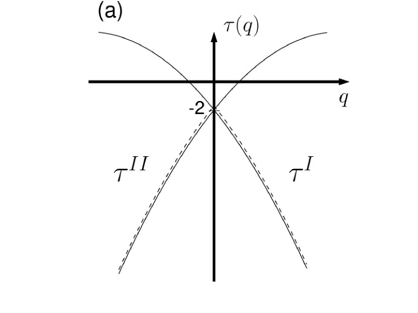
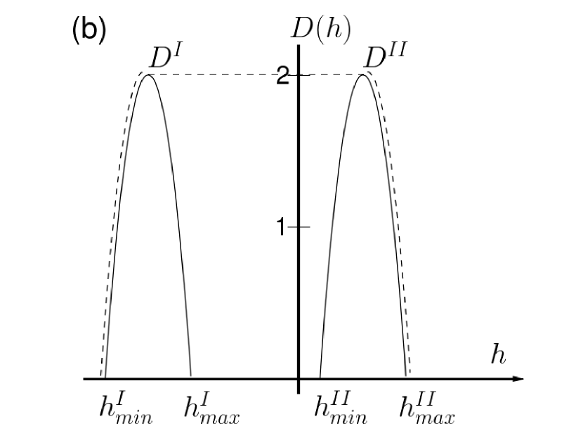
Figure 1: Illustration of a phase transition in the multifractal spectra of a compound system (Eq. (9)). $(\tau^{I}(q),D^{I}(h))$ and $(\tau^{II}(q),D^{II}(h))$ are the multifractal spectra for $f^{I}({\bf x})$ and $f^{II}({\bf x})$ respectively. The 2D WTMM method and more generally the multifractal formalism, give access to the dashed $\tau(q)$ curve (Eq. (11)) in (a) and via the Legendre transform (Eq. (8)) to the dashed $D(h)$ sprectrum in (b) which is the supremum of the $D^{I}(h)$ and $D^{II}(h)$ spectra.

Our segmentation strategy consists in using the WT skeleton to discriminate the maxima lines ${\cal L}^{I}(a)$ associated with singularities of $f^{I}({\bf x})$ and maxima lines ${\cal L}^{II}(a)$ associated with singularities of $f^{II}({\bf x})$, over the range $[a_{min},a_{max}]$ of accessible scales. This can be done theoretically by comparing the power-law behavior of ${\cal M}_{\bf\psi}[f]({\bf x}\in{\cal L})$ along each maxima line of the WT skeleton (Eq. (2)). From the local estimate of $h({\bf x})$, one can expect to partition the WT skeleton into two sub-skeletons, one made of the maxima lines ${\cal L}^{I}(a)$ and the other one made of maxima lines ${\cal L}^{II}(a)$. In practice, this partitioning will suffer from the finite range of scales available to the analysis and the desired segmentation will require special care as far as finite-size effects and statistical convergence issues are concerned.

3 Application of the wavelet-based segmentation method to synthetic data

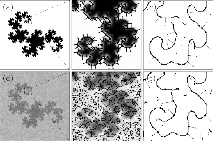
Figure 2: (a) The fractal Dragon ($1024\times 1024$). (b) WTMM chains at the smallest scale $a=\sigma_{W}=7$ pixels in a small $100\times 100$ region of the fractal Dragon. (c) Same as in (b) for scale $a=2\sigma_{W}$. (d) The fractal Dragon embedded in a fractionnal Brownian noise ($H=-0.7$) background of twice as large amplitude. (e) and (f) are the same as (b) and (c) but for the noisy fractal Dragon. In (b,c,e,f), the black arrows represent the WT vectors originating at the WTMMM. In (b) and (e) the background image is the smooth-convoluted image $\phi_{{\bf b},a}*f$ at scale $a=\sigma_{W}$.

We consider an academic example image with two fractal components: the fractal Dragon (Duda, 2007) embedded into a noisy background generated from fractional Brownian noise with Hölder exponent $H=-0.7$. The fractal Dragon is a self-similar fractal defined as the limit set of an iterated function system (the Lindenmayer system) of the same type as the one used to generate the Sierpinski gasket or the Von Koch curve (Mandelbrot, 1982), but the fractal Dragon has less obvious geometrical symmetries. Let us note that the fractal Dragon is space-filling, meaning its fractal dimension is 2, whereas its boundary has a fractal dimension known analytically $D_{Dragon}=\log_{2}(\frac{1+\sqrt[3]{73-6\sqrt{87}}+\sqrt[3]{73+6\sqrt{87}}}{3})\simeq 1.5236$. A sample fractal Dragon is shown in Figure 2(a) whereas the corresponding noisy two-component image is shown in Figure 2(d). As previously discussed, the wavelet analysis proposed in this work is sensitive to singularities, i.e. to points in the images where the signal is singular. We expect the WTMM analysis of the image shown in Fig. 2(d) to simultaneously reveal multifractal information about both the boundary of the fractal Dragon and of the rough background texture. Let us recall that the two components have known mono-fractal type self-similar properties, i.e. a singularity spectrum degenerated to a single point: ($h=-0.7$, $D=2$) for the fractional Brownian noise and ($h=0$, $D=D_{Dragon}\simeq 1.5236$) for the boundary of the fractal Dragon. The roughness $H=-0.7$ of the fractional Brownian noise was chosen to mimic the texture of the quiet-Sun images (see Section 4.1). Figures 2(b) and 2(e) illustrate the results of the computation of the WT maxima chains at the smallest scale; the arrows correspond to the WT vectors (Eq. (1)) at the WTMMM locations. Figures 2(c) and 2(f) show the maxima chains at a scale twice as large as in Figures 2(b) and 2(e). When going from large to small scales, whereas the boundary of the fractal Dragon is better and better approximated by some WTMM chains (edge detection in the smoothed image), an increasing number of additional maxima chains start emerging as the signature of the presence of a colored noise (Fig. 2(e) as compared to Fig. 2(b)).

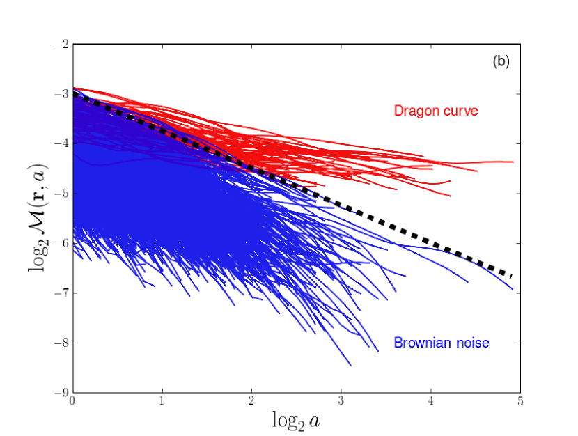
Figure 3: Log-log plot of WT modulus along the skeleton maxima lines versus scale. Lines are colored according to the segmentation procedure (Eq. (12)) : fractal Dragon boundary (red) and fractionnal Brownian noise (blue). (a) Noisy fractal Dragon with a noise amplitude twice as large as the fractal Dragon (see Fig. 2(d)). (b) Noisy fractal Dragon with a noise amplitude five times as large as the fractal Dragon. The dashed black line represents the segmentation condition (Eq. 12).

As previously emphasized (Muzy et al., 1994; Arneodo et al., 1995c, 2003), the set of maxima lines that defines the WT skeleton contains the space-scale information necessary to recover the underlying multifractal properties. In Figures 3(a) and 3(b) are shown in a logarithmic representation, the behavior of the WT modulus along the maxima lines computed for a noisy fractal Dragon with a noise amplitude respectively twice and five times as large as the fractal Dragon. Since the fractional Brownian noise is everywhere singular with Hölder exponent $H=-0.7$ (Mandelbrot, 1982), maxima lines pointing to noise features at small scale are characterized by a WTMMM power law behavior ${\mathcal{M}}_{\boldsymbol{\psi}}[f](a)\sim a^{-0.7}$, while lines associated to the fractal Dragon boundary can be distinguished by the fact that ${\mathcal{M}}_{\boldsymbol{\psi}}[f](a)\sim a^{0}\sim Const$ (no scale dependence). This leads us to implement the following segmentation procedure: the space $(\log_{2}a,\log_{2}{\mathcal{M}}_{\boldsymbol{\psi}}[f](a))$ is divided in two regions separated by a straight line of slope $-0.7<h_{s}<0$ and intercept $\log_{2}M_{s}$. As shown in Figure 3(a), for low noise amplitude, all the maxima lines along which $\log_{2}{\mathcal{M}}_{\boldsymbol{\psi}}[f](a)$ decays slower than $h_{s}\log_{2}a$ when increasing $a$, are colored in red and associated with the Dragon boundary. On the contrary, all the maxima lines along which $\log_{2}{\mathcal{M}}_{\boldsymbol{\psi}}[f](a)$ decays faster than $h_{s}\log_{2}a$ when increasing $a$, are colored in blue and associated with the noise component. But as shown in Figure 3(b), for large noise amplitude the distinction of the two sub-skeletons is much more tricky at small scales where some entangling is observed. We thus adapt the segmentation criteria towards the largest scales in fully analogy with a different but conceptually similar adaptation of the 2D WTMM segmentation method (Khalil et al., 2007). Each maxima line is characterized by a length, i.e. its maximun scale $a_{max}$ and the WT modulus ${\mathcal{M}}_{\boldsymbol{\psi}}[f](a_{max})$ at that scale. A given maxima line is said to belong to the Dragon sub-skeleton, if it satisfies the following condition :

$$\log_{2}{\mathcal{M}}_{\boldsymbol{\psi}}[f](a_{max})\geq h_{s}\log_{2}a_{max}+\log_{2}M_{s}.$$ (12)

Figure 4: Multifractal analysis of the fractal Dragon ($\circ$) and of the noisy ($H=-0.7$) fractal Dragon ($\bullet$) after applying the segmentation procedure (Eq. (12)). (a) $h(q,a)$ vs $\log_{2}a$ for different values of $q$; the solid lines correspond to linear regression fits over the range of scales $a\in[2^{0},2^{4}]~{}\sigma_{W}$ (resp. $[2^{0.5},2^{3.5}]~{}\sigma_{W}$) for the fractal Dragon (resp. the noisy fractal Dragon after segmentation). The symbols (

$\blacksquare$

) correspond to the $h(q=0,a)$ partition function obtained for the noisy fractal Dragon without any segmentation. (b) $D(q,a)$ vs $\log_{2}a$. (c) $\tau(q)$ vs $q$; the dashed horizontal line is the theoretical spectrum $\tau(q)=-1.5236$ ($\forall q$) of the boundary of the fractal Dragon. (d) $D(h)$ vs $h$; the symbols ($\bullet$) correspond to the segmented $D(h)$ spectrum for the fractal Dragon component; the ($\times$) correspond to the extracted $D(h)$ spectrum of the colored noisy background. The zoom-in window enlarges $D(h)$ data corresponding to the noisy fractal Dragon ($\bullet$) after applying the segmentation procedure.

In Figures 4(a) and 4(b) are reported the results of the computation of the partition functions for the fractal Dragon alone and its noisy version after applying the segmentation condition (Eq. (12)) with $h_{s}=-0.5$ and $\log_{2}M_{s}=-3.2$. In Figure 4(a), the partition functions $h(q,a)$ (Eq. (5)) of the noisy Dragon display a well defined scaling behavior over 3 octaves (compared to 4 octaves for the original fractal Dragon), for a wide range of values of $q\in[-2,3]$. For negative $q$ values, at very small scales, the segmentation procedure fails to disentangle the two components due to the contribution from the noisy component with $h(q)\simeq-0.7$. Nevertheless the gain in scaling is unquestionable as compared to the behavior of the $h(q,a)$ partition functions without segmentation (the $\blacksquare$ in Fig. 4(a)). Without any segmentation the partition functions are a mixture of different scaling behaviors from which reliable quantitative information cannot be extracted. In Figures 4(c) and 4(d) are shown the corresponding $\tau(q)$ and $D(h)$ spectra. Despite some slight departure from monofractality for the segmented noisy fractal Dragon (that is also observed but to a lesser extent in the original fractal Dragon as the result of finite-size effects), one recovers a rather good estimate of the fractal dimension $D_{F}=1.57\pm 0.03$ of the fractal Dragon boundary. Furthermore, as reported in Figure 4(d), our segmentation procedure has proved to be very efficient to estimate separately the $D(h)$ singularity spectra of both the fractal Dragon and the noisy background. This efficiency is illustrated in Figure 5

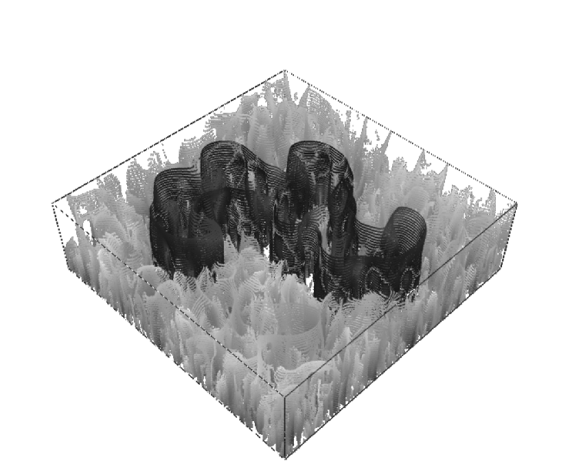
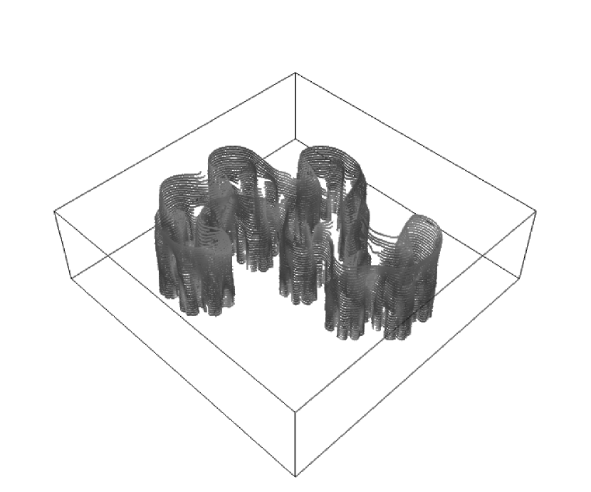
Figure 5: 3D visualization in the space-scale $(x,y,scale)$ representation of the WTMM chains computed from the image shown in Fig. 2(d) before (a) and after (b) the segmentation procedure (Eq. (12)). At each scale $a$, only the maxima chains containing at least one WTMMM belonging to the resulting WT skeleton are displayed.

where a 3D $(x,y,scale)$ space-scale visualization of the maxima chains of the noisy Dragon prior (Fig. 5(a)) and after (Fig. 5(b)) segmentation clearly confirms the elimination of noise-induced small scale features that would otherwise severely affect the multifractal analysis.

4 Application of the wavelet-based segmentation method to Solar magnetogram data

Magnetic field measurements were obtained by the Michelson Doppler Imager (MDI) on the Solar and Heliospheric Observatory (SOHO), which images the Sun on a 1024$\times$1024 pixel CCD camera through a series of increasingly narrow filters (Scherrer et al., 1995). The final elements, a pair of tunable Michelson interferometers, enable MDI to record filtergrams with an FWHM bandwidth of 94 mÅ. In this paper, 96-minute magnetograms of the full disc were used, which had a pixel size of $\sim$2”. For the purposes of this work, a series of magnetograms have been analyzed to examine the difference in fractal properties between quiet and active solar regions. A total of 29 magnetograms representative of the quiet Sun were taken from December 21 to December 22, 2006 and a similar series of 28 images representative of the active Sun were taken from October 27 to October 29, 2003. In the solar photosphere, the large magnetic Reynolds number ($\sim 10^{7}-10^{9}$) means that magnetic field lines will be advected with the flow of plasma (McAteer et al., 2009). This system naturally leads to self-similarity, suggesting a multifractal study is appropriate (Lawrence et al., 1993; Abramenko et al., 2002; McAteer et al., 2005). As already mentioned, previous method of calculating the multifractal properties of solar magnetic features are dependent on image resolution, thresholding, and instrument sensitivity. The WTMM method calculates the multifractal spectrum of solar magnetic features based on the distribution of gradients within the image at various scales. As such, the WTMM multifractal parameters are less sensitive to changes in image resolution and instruments than traditional methods.

4.1 Quiet-Sun multifractal properties

Figure 6: (Top, Left) MDI magnetogram taken on December 20, 2006; (Top, Right) MDI magnetogram taken on October 28, 2003. (Bottom) Histogram values of the wavelet transform modulus ${\mathcal{M}}_{\boldsymbol{\psi}}[f](a)$ at the smallest scale ($\sigma_{W}=7$ pixels) for MDI magnetogram images of a quiet Sun (solid) and active Sun (dashed).

Examples of quiet and active MDI magnetograms analyzed are shown in Figure 6 (top left and top right respectively), with a histogram of the wavelet transform modulus ${\mathcal{M}}_{\boldsymbol{\psi}}[f]({\bf b},a)$ at the smallest scale (bottom). Active regions result from an increased proportion of large magnetic elements of opposite polarity in close proximity to each other. The resulting neutral or magnetic inversion lines can be detected using standard wavelet-based techniques (Ireland et al., 2008). As such active regions should contain a greater number of higher magnitude WT gradients. This is shown in Figure 6 (bottom), which suggests that moduli with values larger than $40$ are unlikely in quiet-Sun magnetograms. Due to the different scaling properties of active regions and their surrounding quiet Sun, our goal is to segment the WT skeletons using the condition defined in Eq. (12). As outlined in Section 2 and illustrated on synthetic data in Section 3, this should allow us to study the multifractal properties of active regions in a quantitative manner.

Figure 7: Multifractal analysis of a set of 30 quiet-Sun images (505$\times$505) prior ($\circ$) and after (

$\blacksquare$

) thresholding (a sample thresholded magnetogram is shown in Figure 8). (a) $\log_{2}h(q,a)$ vs $\log_{2}a$ for different values of $q$; the solid lines are linear regression fits over the range of scales $a\in[2^{0},2^{3.7}]~{}\sigma_{W}$. (b) $\log_{2}D(q,a)$ vs $\log_{2}a$. (c) $\tau(q)$ vs $q$; the dashed straight line is the theoretical linear spectrum $\tau(q)=-0.75q-2$ of the 2D fractional Brownian noise with Hölder exponent $H=-0.75$. (d) $D(h)$ vs $h$; the dashed lines delimit the position of the top of the $D(h)$ curves. Error bars correspond to standard deviation in the linear regression procedure.

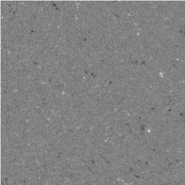
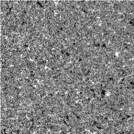
Figure 8: 256$\times$256 quiet-Sun images. Image on the right is a threshholded version of the left one. Pixels with large absolute magnetic flux are shrinked down. Multifractal properties of quiet-Sun images and the corresponding thresholded versions are shown in Figure 7.

The results of the computation of the multifractal spectra when averaging the partition functions over a set of 30 ($505\times 505$) quiet-Sun images without applying the segmentation are reported in Figure 7. As shown in Figure 7(a) and 7(b), $h(q,a)$ (Eq. (5)) and $D(q,a)$ (Eq. (6)) display convincing scaling behavior over almost four octaves for $q\in[-2,3]$ (symbol ($\circ$)). Linear regression fits of the data yield the non-linear $\tau(q)$ spectrum shown in Figure 7(c). This multifractal diagnosis can also be observed in Figure 7(a) where the slope $h(q)$ of the partition function $h(q,a)$ versus $\log_{2}a$ definitely depends on $q$. The corresponding multifractal spectrum $D(h)$ is shown in Figure 7(d). From the top of the $D(h)$ curve, we can see that quiet-Sun images are everywhere singular ($D(q=0)=2$) with a corresponding Hölder exponent $h(q=0)\simeq-0.75$. The multifractality can be quantified by the so-called intermittency coefficient $c_{2}$ that characterizes the width of the $D(h)$ curve. As shown in Figures 7(c) and 7(d), the $\tau(q)$ and $D(h)$ data of the quiet-Sun images are well fitted by a parabola

$$\tau(q)=-c_{0}+c_{1}q-\frac{c_{2}}{2}q^{2},\;\;\;\;\;\;D(h)=c_{0}-\frac{(h-c_{1})^{2}}{2c_{2}},$$ (13)

where $c_{0}\simeq 2$, $c_{1}\simeq-0.75$ and $c_{2}\simeq 0.22$. Let us point out that quadratic multifractal spectra are predicted by the so-called log-normal model that has been popularized by the fully-developed turbulence community (Frisch, 1995; Arneodo et al., 1998a, 1999b; Delour et al., 2001). In the present case, there is no particular evidence of the relevance of this model except that the observed $\tau(q)$ and $D(h)$ multifractal spectra are well characterized by their log-normal quadratic approximations.

In order to understand the source of this intermittency, a upper threshold was imposed on each MDI magnetogram of the quiet Sun (Figure 8). The threshold operation has the effect of removing large magnetic features resting on the boundary of the super-granular structures of the Sun. In Figure 7(d), we can see that the multifractality of the thresholded quiet-Sun image (symbol $\blacksquare$ ) set is strongly reduced but not totally cancelled. We can also note that the average Hölder exponent is slightly shifted from $<h>=c_{1}=-0.75$ to $-0.82$, and the intermittency coefficient is reduced to $c_{2}\sim 0.06$ (Let us recall that a value $c_{2}=0$ means that the underlying process is monofractal). Without the super-granular magnetic structure, the quiet-Sun multifractal spectrum looks much more monofractal. This suggests that the magnetic features resting on the boundaries of the super-granular structure are a major actor in the observed intermittent structural properties of the Sun (Georgoulis et al., 2002). Since current models for the solar dynamo use information on the fractal dimension of solar disk as a whole (Pontieri et al., 2003), these new informations on the photosphere and the characteristic make-up of the quiet Sun should be incorporated in further theoretical works.

4.2 Solar magnetogram active region segmentation

In this section, we highlight the use of the WTMM segmentation method on Solar magnetogram data with active regions, to demonstrate its ability to analyze the underlying multifractal properties of the active regions that are embedded in the surrounding quiet-Sun texture.

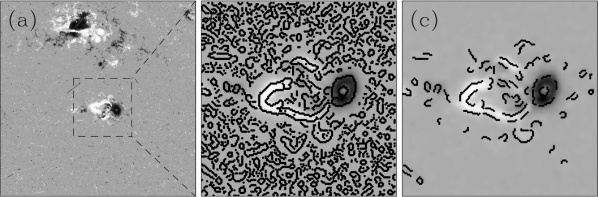
Figure 9: (a) 505$\times$505 Active Region example image (October 28, 2003). (b) WTMM chains at the smallest scale ($a=\sigma_{W}$ pixels) in a small $150\times 150$ region surrounding an active spot. (c) WTMM chains left after the segmentation step.

A sample $505\times 505$ magnetogram MDI image containing an active region is shown in Figure 9. Figures 9(b) and 9(c) show respectively the results of the computation of the WTMM chains before and after the segmentation at scale $a=\sigma_{W}\sim 7$ pixels of a small $150\times 150$ excerpt focused on the active location. As explained in Section 4.1, WT skeleton maxima lines associated with quiet-Sun structures have a characteristic scaling behavior described by ${\mathcal{M}}_{\boldsymbol{\psi}}[f](a)\sim a^{-0.7}$. This behavior is used to derive the parameters characterizing the line $l_{2}$ in Figure 10

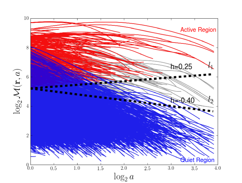
Figure 10: Log-log plot of the WT modulus along the skeleton maxima lines versus scale. The dashed line denoted $l_{1}$ with slope $h_{A}=0.25$ and intercept $\log_{2}M_{A}=5.2$ is used to identify WT skeleton maxima lines associated to the active region (red). According to Eq. (15), these lines have an ending point at highest scale ($\log_{2}a_{max},\log_{2}{\mathcal{M}}_{\boldsymbol{\psi}}[f](\mathbf{r},a_{max})$) above $l_{1}$. The dashed line denoted $l_{2}$ with slope $h_{Q}=-0.40$ and intercept $\log_{2}M_{Q}=5.2$ is used to identify maxima lines associated to the quiet Sun (blue). According to Eq. (14), these lines have an ending point below $l_{2}$. All other lines (grey) are not clearly identified to belong either to the active site or the quiet surrounding. The values of the segmentation parameters $h_{A}$, $\log_{2}M_{A}$, $h_{Q}$ and $\log_{2}M_{Q}$ were chosen by examining the WTMM histogram at the smallest scale to extract at best a sub-skeleton specific to the active region.

that will allow us to discriminate in the WT skeleton, the maxima lines (blue) that correspond to quiet-Sun structures:

$$\log_{2}{\mathcal{M}}_{\boldsymbol{\psi}}[f](a_{max})\leq h_{Q}\log_{2}a_{max}+\log_{2}M_{Q},$$ (14)

where $-0.7<h_{Q}<0$, so that for the selected maxima lines $\log_{2}{\mathcal{M}}_{\boldsymbol{\psi}}[f](a)$ will decrease fast enough when increasing the scale $a$ to correspond to the quiet phase. To select the maxima lines (red) associated with the active region, we use another separating line $l_{1}$ in Figure 10:

$$\log_{2}{\mathcal{M}}_{\boldsymbol{\psi}}[f](a_{max})\geq h_{A}\log_{2}a_{max}+\log_{2}M_{A},$$ (15)

where this time $0\leq h_{A}<0.38$, to limit the decrease (if any) of $\log_{2}{\mathcal{M}}_{\boldsymbol{\psi}}[f]$ when increasing $a$. Note that the lines $l_{1}$ and $l_{2}$ have different slopes because some maxima lines cannot be clearly associated with either the quiet Sun or the active region state. Indeed those maxima lines are associated to features located near the boundary between quiet-Sun and active regions. When going from small scales to large scales the support of the analyzing wavelet starts covering partly both regions preventing accurate classification. As illustrated in Figure 11, when fixing the segmentation parameters to $h_{Q}=-0.40$, $h_{A}=0.25$ and $\log_{2}M_{Q}=\log_{2}M_{A}=5.2$, the space-scale nature of the methodology allows us to disentangle maxima chains associated with the active region from those corresponding to the quiet Sun. Let us note that in a future work on large data sets, an automated parameters adjustment will be implemented using a clustering algorithm. In addition, a wrong choice of segmentation parameters can be observed in the partition function plots (not shown here) which display a phase transition phenomenon, i.e. a scaling behavior that changes from one state to the other when going from small scales to large scale due to to non-homogenous phases and mis-classified maxima lines.

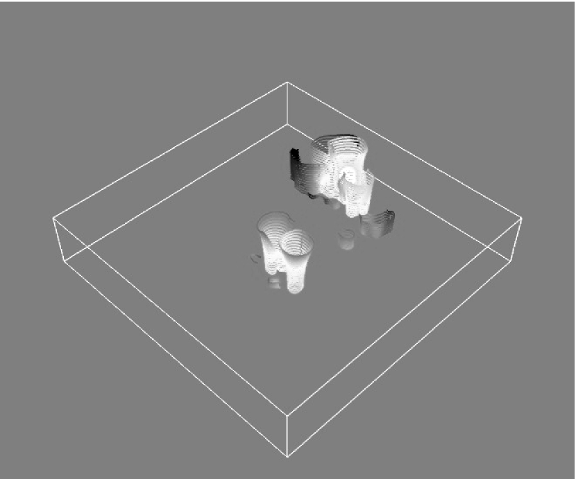
Figure 11: 3D visualization in the space-scale $(x,y,scale)$ representation of the WTMM chains computed from the image shown in Fig. 9(a) before (left) and after (right) the segmentation procedure. The segmentation conditions are defined in Figure 10. The maxima chains displayed contain at least one WTMMM belonging to the resulting skeleton.

Figure 12: Multifractal analysis of a set of 5 active region magnetogram images (505$\times$505) corresponding to the two sub-skeletons identified in Figures 10 and 11. The symbols ($\bullet$) correspond to the segmented quiet Sun and ($\circ$) to the segmented active region. (a) $h(q,a)$ vs $\log_{2}a$ for different values of $q$; the solid lines are linear regression fits over the range of scales $a\in[2^{0},2^{3.0}]~{}\sigma_{W}$. (b) $D(q,a)$ vs $\log_{2}a$. (c) $\tau(q)$ vs $q$. (d) $D(h)$ vs $h$. Error bars correspond to standard deviations in the linear regression procedure.

In Figure 12 are shown the results of the partition function computation for a set of 5 active region magnetogram images taken on October 28^th, 2003 (one image out of this set is shown in Figure 9(a)). Partition functions are computed separately for each sub-skeleton corresponding to the extracted action region maxima lines and quiet-Sun maxima lines shown in Figure 10. From these plots, one can see that the $\log_{2}h(q,a)$ versus $\log_{2}a$ data are nicely modeled with linear regression fits with slope $h(q)$ that depends on $q$ as the signature of multifractal scaling. This demonstrates that the segmentation procedure successfully extracts from the magnetogram images two scale invariant components with different multifractal properties. The $\tau(q)$ (Fig. 12(c)) and $D(h)$ (Fig. 12(d)) spectra computed from the set of quiet-Sun maxima lines (blue lines in Fig. 10) are in good agreement with the ones previously computed in Section 4.1 from pure quiet-Sun images (Figs. 7(c) and 7(d) respectively). Using the log-normal approximation (Eq. (13)), we get $c_{0}=2$, $c_{1}=-0.65$ and $c_{2}=0.10$. This means that the extracted quiet Sun appears (like the thresholded MDI magnetograms of quiet Sun in Figs 7(c) and 7(d)) a little less intermittent as compared to the previous estimate $c_{2}=0.22$. As for the active region, the corresponding partition functions computed from the set of active phase maxima lines (red lines in Fig. 10) display very convincing multifractal scaling behavior as quantified by the $\tau(q)$ and $D(h)$ spectra shown in Figures 12(c) and 12(d) respectively. Again these spectra are well approximated by the quadratic log-normal formula (Eq. (13)) with parameters $c_{0}=2$, $c_{1}=0.38$ and $c_{2}=0.12$. This indicates that the singularities associated with the active region are space-filling (they are distributed on a set of fractal dimension $D_{F}=c_{0}=2$), with a mean strength $h(q=0)=c_{1}=0.38$ meaning that magnetogram images can be considered as continuous on active regions (over the range of scales of our analysis) but noisy on quiet regions.

5 Conclusions

Many complex physical systems analyzed using fractal and multifractal techniques are surrounded or embedded in a noisy background sometimes originating from instrumental noise. As such these systems are a statistical combination of two distinct self-similar structures. This work addressed the need for an accurate calculation of the multifractal parameters of such complex systems. The presence of compound scale-invariant structures can result in an inaccurate or skewed calculation of the fractal and multifractal parameters when studied as a whole. Using a wavelet-based multi-scale segmentation method, we show that it is possible to disentangle to some extent these two processes and accurately (up to finite-size effects) recover the multifractal characteristics of the system of interest. A theoretical test example for this method was provided in section 2. The removal of information relating to the background noise was highlighted in Figure 5. The quantitative results reported in Figure 4 attest of the ability of this segmentation method to recover the multifractal parameters in question.

Let us emphasize here that the application of this method to experimental data for which we do not have a priori knowledge of the possible underlying multifractal processes is a difficult task that requires much attention to perform the most objective segmentation which can not be infered or guided by some physical rule or information. The multifractal analysis is a statistical tool that has direct connections with signal and image processing, but not necessarily with the physics of the system per se. As noticed in section 4.2, the use of a clustering algorithm should greatly help in adjusting the multifractal parameters of the differents components as well as in providing an automated procedure for processing large data sets. This will be reported in a future publication.

The application of this wavelet-based methodology to quiet-Sun data has revealed the multifractal nature of this intermittent noisy component ($<h>=-0.75$) as mainly resulting from the super-granular magnetic structures. The quiet-Sun study was also necessary to get expertise for further analyzing more complex images that involve a segmentation before being able to clearly identify the underlying multifractal properties. We have checked that the partition functions computations for the segmented quiet-Sun phase provide (i) convincing scaling properties and (ii) multifractal spectra $\tau(q)$ and $D(h)$ estimates in good numerical agreement with the one measured in the previous calibration step. The assumption of two non-overlapping $D(h)$ is not inconsistent with the data. Let us notice that a phase transition can be observed in the partition function log-log plots when inappropriate segmentation parameters are chosen. In the case of overlapping $D(h)$, there would be a large set of maxima lines in the WT skeleton that could not be genuinely sorted, which would prevent from building accurate multifractal $D(h)$ measurement. From the analyzed data, we were not able to distinguish more than two phases. Finally, this gives us good confidence in the segmentation proposed for solar magnetogram containing an active region. However, further study is needed to precisely quantify scaling properties associated to specific active region features (e.g. emerging magnetic flux along the main polarity inversion line, sunspots build-up, delta-configuration…) and how the WTMM method can be sensitive to these elements. More precisely, when analyzing higher resolution images than MDI, we expect that this segmentation tool will be all the more necessary as quiet-Sun and active region features are more entangled.

The main outcome of the present study is the demonstration that the proposed multi-scale segmentation procedure provides an objective way of studying the complexity in active regions separately from the surrounding quiet Sun. As such our results are significantly more stable and robust when compared to previous fractal and multifractal analysis (Pontieri et al., 2003; McAteer et al., 2005). In a forthcoming paper, we will report on the application of this segmentation method to characterize the evolution of active regions keeping track of the multifractal parameters for possible correlations with extreme solar events (Gallagher et al., 2007). Other applications of this method are in progress as the analysis of the intrinsic multifractal properties of entangled hot and cold interstellar atomic gas from 3D numerical simulations (Kestener & Audit, 2009).

References

- Abramenko et al. (2002) Abramenko, V., Yurchyshyn, V., Wang, H., Spirock, T., & Goode, P. 2002, ApJ, 577, 487
- Aharony & Feder (1989) Aharony, A. & Feder, J., eds. 1989, Fractals in Physics, Essays in honour of B.B. Mandelbrot, Physica D, Vol. 38 (Amsterdam: North-Holland)
- Argoul et al. (1990) Argoul, F., Arneodo, A., Elezgaray, J., Grasseau, G., & Murenzi, R. 1990, Phys. Rev. A, 41, 5537
- Arneodo et al. (1995a) Arneodo, A., Argoul, F., Bacry, E., Elezgaray, J., & Muzy, J. F. 1995a, Ondelettes, Multifractales et Turbulences : de l’ADN aux croissances cristallines (Paris: Diderot Editeur, Art et Sciences)
- Arneodo et al. (1992a) Arneodo, A., Argoul, F., Bacry, E., Muzy, J. F., & Tabard, M. 1992a, Phys. Rev. Lett., 68, 3456
- Arneodo et al. (1992b) Arneodo, A., Argoul, F., Muzy, J. F., & Tabard, M. 1992b, Physica A, 188, 217
- Arneodo et al. (1992c) Arneodo, A., Argoul, F., Muzy, J. F., & Tabard, M. 1992c, Phys. Lett. A, 171, 31
- Arneodo et al. (2002) Arneodo, A., Audit, B., Decoster, N., Muzy, J. F., & Vaillant, C. 2002, The Science of Disasters : climate disruptions, heart attacks and market crashes, ed. A. Bunde, J. Kropp, & H. J. Schellnhuber (Berlin: Springer Verlag), 27
- Arneodo et al. (1995b) Arneodo, A., Bacry, E., Graves, P. V., & Muzy, J. F. 1995b, Phys. Rev. Lett., 74, 3293
- Arneodo et al. (1995c) Arneodo, A., Bacry, E., & Muzy, J. F. 1995c, Physica A, 213, 232
- Arneodo et al. (1996) Arneodo, A., d’Aubenton-Carafa, Y., Bacry, E., et al. 1996, Physica D, 96, 291
- Arneodo et al. (2003) Arneodo, A., Decoster, N., Kestener, P., & Roux, S. G. 2003, in Advances in Imaging and Electron Physics, Vol. 126, (San Diego: Academic Press), 1
- Arneodo et al. (1999a) Arneodo, A., Decoster, N., & Roux, S. G. 1999a, Phys. Rev. Lett., 83, 1255
- Arneodo et al. (2000) Arneodo, A., Decoster, N., & Roux, S. G. 2000, Eur. Phys. J. B, 15, 567
- Arneodo et al. (1998a) Arneodo, A., Manneville, S., & Muzy, J. F. 1998a, Eur. Phys. J. B, 1, 129
- Arneodo et al. (1999b) Arneodo, A., Manneville, S., Muzy, J. F., & Roux, S. G. 1999b, Phil. Trans. R. Soc. London A, 357, 2415
- Arneodo et al. (1998b) Arneodo, A., Muzy, J. F., & Sornette, D. 1998b, Eur. Phys. J. B, 2, 277
- Arrault et al. (1997) Arrault, J., Arneodo, A., Davis, A., & Marshak, A. 1997, Phys. Rev. Lett., 79, 75
- Audit et al. (2001) Audit, B., Thermes, C., Vaillant, C., et al. 2001, Phys. Rev. Lett., 86, 2471
- Audit et al. (2002) Audit, B., Vaillant, C., Arneodo, A., d’Aubenton-Carafa, Y., & Thermes, C. 2002, J. Mol. Biol., 316, 903
- Bacry et al. (1993) Bacry, E., Muzy, J. F., & Arneodo, A. 1993, J. Stat. Phys., 70, 635
- Bohr & Tèl (1988) Bohr, T. & Tèl, T. 1988, in Direction in Chaos, ed. B. L. Hao, Vol. 2 (Singapore: World Scientific), 194
- Brodie of Brodie et al. (2005) Brodie of Brodie, E., Nicolay, S., Touchon, M., et al. 2005, Phys. Rev. Lett., 94, 248103
- Bunde & Havlin (1994) Bunde, A. & Havlin, S., eds. 1994, Fractals in Science, hardcover edn. (Berlin: Springer)
- Bunde et al. (2002) Bunde, A., Kropp, J., & Schellnhuber, H. J., eds. 2002, The Science of Disasters : climate disruptions, heart attacks and market crashes (Berlin: Springer Verlag)
- Caddle et al. (2007) Caddle, L. B., Grant, J. L., Szatkiewicz, J., et al. 2007, Chromosome Res, 15, 1061
- Collet et al. (1987) Collet, P., Lebowitz, J., & Porzio, A. 1987, J. Stat. Phys., 47, 609
- Conlon et al. (2008) Conlon, P. A., Gallagher, P. T., McAteer, R. T. J., et al. 2008, Sol. Phys., 248, 297
- Daubechies (1992) Daubechies, I. 1992, Ten Lectures on Wavelets, CBMS-NSF Regional Conference Series in Applied Mathematics (Philadelphia: SIAM)
- Decoster et al. (2000) Decoster, N., Roux, S. G., & Arneodo, A. 2000, Eur. Phys. J. B, 15, 739
- Delour et al. (2001) Delour, J., Muzy, J. F., & Arneodo, A. 2001, Eur. Phys. J. B, 23, 243
- Duda (2007) Duda, J. 2007, Complex base numeral systems
- Family et al. (1995) Family, F., Meakin, P., Sapoval, B., & Wool, R., eds. 1995, Fractal Aspects of Materials, Material Research Society Symposium Proceeding, Vol. 367 (Pittsburg)
- Feder (1988) Feder, J. 1988, Fractals (New York: Pergamon)
- Frisch (1995) Frisch, U. 1995, Turbulence (Cambridge: Cambridge Univ. Press)
- Gallagher et al. (2007) Gallagher, P. T., McAteer, R. T. J., Young, C. A., et al. 2007, in Astrophysics and Space Science Library, Vol. 344, Space Weather : Research Towards Applications in Europe 2nd European Space Weather Week (ESWW2), ed. J. Lilensten, 15
- Georgoulis et al. (2002) Georgoulis, M., Rust, D., Bernasconi, P., & Schmieder, B. 2002, ApJ, 575, 506
- Georgoulis (2005) Georgoulis, M. K. 2005, Sol. Phys., 228, 5
- Goupillaud et al. (1984) Goupillaud, P., Grossmann, A., & Morlet, J. 1984, Geoexploration, 23, 85
- Grassberger et al. (1988) Grassberger, P., Badii, R., & Politi, A. 1988, J. Stat. Phys., 51, 135
- Grassberger & Procaccia (1983a) Grassberger, P. & Procaccia, I. 1983a, Phys. Rev. Lett., 50, 346
- Grassberger & Procaccia (1983b) Grassberger, P. & Procaccia, I. 1983b, Physica D, 9, 189
- Grossmann & Morlet (1984) Grossmann, A. & Morlet, J. 1984, S.I.A.M. J. Math. Anal., 15, 723
- Halsey et al. (1986) Halsey, T. C., Jensen, M. H., Kadanoff, L. P., Procaccia, I., & Shraiman, B. I. 1986, Phys. Rev. A, 33, 1141
- Hentschel (1994) Hentschel, H. G. E. 1994, Phys. Rev. E, 50, 243
- Ireland et al. (2008) Ireland, J., Young, C. A., McAteer, R. T. J., et al. 2008, Sol. Phys., 252, 121
- Ivanov et al. (1999) Ivanov, P. C., Nunes Amaral, L. A., Goldberger, A. L., et al. 1999, Nature, 399, 461
- Ivanov et al. (1996) Ivanov, P. C., Rosenblum, M. G., Peng, C. K., et al. 1996, Nature, 383, 323
- Jaffard (1997) Jaffard, S. 1997, SIAM J. Math. Anal., 28, 944; ibid. 28, 971
- Jaffard et al. (2006) Jaffard, S., Lashermes, B., & Abry, P. 2006, in Wavelet Analysis and Applications, ed. T. Qian, M. I. Vai, & Y. Xu (Basel, Switzerland,: Birkhäuser Verlag), 219
- Kestener & Arneodo (2003) Kestener, P. & Arneodo, A. 2003, Phys. Rev. Lett., 91, 194501
- Kestener & Arneodo (2004) Kestener, P. & Arneodo, A. 2004, Phys. Rev. Lett., 93, 044501
- Kestener & Arneodo (2007) Kestener, P. & Arneodo, A. 2007, Stoch. Environ. Res. Risk Assess., 22, 421
- Kestener & Audit (2009) Kestener, P. & Audit, E. 2009, In preparation
- Kestener et al. (2001) Kestener, P., Lina, J. M., Saint-Jean, P., & Arneodo, A. 2001, Image Anal. Stereol., 20, 169
- Khalil et al. (2007) Khalil, A., Grant, J. L., Caddle, L. B., et al. 2007, Chromosome Res., 15, 899
- Khalil et al. (2006) Khalil, A., Joncas, G., Nekka, F., Kestener, P., & Arneodo, A. 2006, ApJS, 165, 512
- Khalil et al. (2009) Khalil, A., Mason, M., Dickey, I., et al. 2009, Medical Engineering and Physics, 31, 775
- Kuhn et al. (1994) Kuhn, A., Argoul, F., Muzy, J. F., & Arneodo, A. 1994, Phys. Rev. Lett., 73, 2998
- Lawrence et al. (1993) Lawrence, J., Ruzmaikin, A., & Cadavid, A. 1993, ApJ, 417, 805
- Lea-Cox & Wang (1993) Lea-Cox, B. & Wang, J. S. Y. 1993, Fractals, 1, 87
- Mallat (1998) Mallat, S. 1998, A Wavelet Tour in Signal Processing (New York: Academic Press)
- Mallat & Hwang (1992) Mallat, S. & Hwang, W. L. 1992, IEEE Trans. on Information Theory, 38, 617
- Mallat & Zhong (1992) Mallat, S. & Zhong, S. 1992, IEEE Trans. on Pattern Analysis and Machine Intelligence, 14, 710
- Mandelbrot (1974) Mandelbrot, B. B. 1974, J. Fluid Mech., 62, 331
- Mandelbrot (1982) Mandelbrot, B. B. 1982, The Fractal Geometry of Nature (San Francisco: Freeman)
- Mandelbrot (1989) Mandelbrot, B. B. 1989, Selecta, Vol. 1, Fractals and Multifractals : Noise, Turbulence and Galaxies (Berlin: Springer Verlag)
- McAteer et al. (2005) McAteer, R., Gallagher, P., & Ireland, J. 2005, ApJ, 631, 628
- McAteer et al. (2007) McAteer, R., Young, C., Ireland, J., & Gallagher, P. 2007, ApJ, 662, 691
- McAteer et al. (2009) McAteer, R. J., Gallagher, P. T., & Conlon, P. A. 2009, Advances in Space Research, In Press, Corrected Proof,
- Meneveau & Sreenivasan (1991) Meneveau, C. & Sreenivasan, K. R. 1991, J. Fluid Mech., 224, 429
- Meyer (1990) Meyer, Y. 1990, Ondelettes (Paris: Herman)
- Monin & Yaglom (1975) Monin, A. S. & Yaglom, A. M. 1975, Statistical Fluid Mechanics, Vol. 2 (Cambridge, MA: MIT Press)
- Muzy et al. (1991) Muzy, J. F., Bacry, E., & Arneodo, A. 1991, Phys. Rev. Lett., 67, 3515
- Muzy et al. (1993) Muzy, J. F., Bacry, E., & Arneodo, A. 1993, Phys. Rev. E, 47, 875
- Muzy et al. (1994) Muzy, J. F., Bacry, E., & Arneodo, A. 1994, Int. J. of Bifurcation and Chaos, 4, 245
- Muzy et al. (2000) Muzy, J. F., Sornette, D., Delour, J., & Arneodo, A. 2000, Quantitative Finance, 1, 131
- Nicolay et al. (2007) Nicolay, S., Brodie of Brodie, E. B., Touchon, M., et al. 2007, Phys. Rev. E, 75, 032902
- Paladin & Vulpiani (1987) Paladin, G. & Vulpiani, A. 1987, Phys. Rep., 156, 148
- Parisi & Frisch (1985) Parisi, G. & Frisch, U. 1985, in Turbulence and Predictability in Geophysical Fluid Dynamics and Climate Dynamics, ed. M. Ghil, R. Benzi, & G. Parisi, Proc. of Int. School (Amsterdam: North-Holland), 84
- Peitgen & Saupe (1987) Peitgen, H. O. & Saupe, D., eds. 1987, The Science of Fractal Images (New York: Springer Verlag)
- Pontieri et al. (2003) Pontieri, A., Lepreti, F., Sorriso-Valvo, L., Vecchio, A., & Carbone, V. 2003, Sol. Phys., 213, 195
- Rand (1989) Rand, D. 1989, Ergod. Th. and Dyn. Sys., 9, 527
- Roland et al. (2009) Roland, T., Khalil, A., Tanenbaum, A., et al. 2009, Surface Science, 603, 3307
- Roux et al. (2000) Roux, S. G., Arneodo, A., & Decoster, N. 2000, Eur. Phys. J. B, 15, 765
- Roux et al. (1999) Roux, S. G., Muzy, J. F., & Arneodo, A. 1999, Eur. Phys. J. B, 8, 301
- Roux et al. (2009) Roux, S. G., Venugopal, V., Fienberg, K., Arneodo, A., & Foufoula-Georgiou, E. 2009, Advances in Water Resources, 32, 41
- Scherrer et al. (1995) Scherrer, P. H., Bogart, R. S., Bush, R. I., et al. 1995, Sol. Phys., 162, 129
- Snow et al. (2008a) Snow, C., Goody, M., Kelly, M., et al. 2008a, PLoS Genetics, 4, e1000219
- Snow et al. (2008b) Snow, C., Peterson, M., Khalil, A., & Henry, C. 2008b, Dev. Dyn., 237, 2542
- Taqqu et al. (1995) Taqqu, M. S., Teverovsky, V., & Willinger, W. 1995, Fractals, 3, 785
- Taylor et al. (2003) Taylor, A. R., Gibson, S. J., Peracaula, M., et al. 2003, AJ, 125, 3145
- Touchon et al. (2005) Touchon, M., Nicolay, S., Audit, B., et al. 2005, Proc. Natl. Acad. Sci. USA, 102, 9836
- Venugopal et al. (2006a) Venugopal, V., Roux, S. G., Foufoula-Georgiou, E., & Arneodo, A. 2006a, Water Resour. Res., 42, W06D14
- Venugopal et al. (2006b) Venugopal, V., Roux, S. G., Foufoula-Georgiou, E., & Arneodo, A. 2006b, Phys. Lett. A, 348, 335
- Vicsek et al. (1994) Vicsek, T., Schlesinger, M., & Matsushita, M., eds. 1994, Fractals in Natural Science (Singapore: World Scientific)
- Wendt & Abry (2007) Wendt, H. & Abry, P. 2007, IEEE Transactions on Signal Processing, 55, 4811
- Wendt et al. (2007) Wendt, H., Abry, P., & Jaffard, S. 2007, IEEE Signal Processing Magazine, 24, 38
- West (1990) West, B. J. 1990, Fractal Physiology and Chaos in Medecine (Singapore: World Scientific)
- Wilkinson et al. (1995) Wilkinson, G. G., Kanellopoulos, J., & Megier, J., eds. 1995, Fractals in Geoscience and Remote Sensing, Image Understanding Research Series, vol.1, ECSC-EC-EAEC (Luxemburg: Brussels)