Improving Semi-Supervised Support Vector Machines
Through Unlabeled Instances Selection

Abstract

Semi-supervised support vector machines (S3VMs) are a kind of popular approaches which try to improve learning performance by exploiting unlabeled data. Though S3VMs have been found helpful in many situations, they may degenerate performance and the resultant generalization ability may be even worse than using the labeled data only. In this paper, we try to reduce the chance of performance degeneration of S3VMs. Our basic idea is that, rather than exploiting all unlabeled data, the unlabeled instances should be selected such that only the ones which are very likely to be helpful are exploited, while some highly risky unlabeled instances are avoided. We propose the S3VM-us method by using hierarchical clustering to select the unlabeled instances. Experiments on a broad range of data sets over eighty-eight different settings show that the chance of performance degeneration of S3VM-us is much smaller than that of existing S3VMs.

[cor1]Corresponding author. Email: zhouzh@nju.edu.cn

1 Introduction

In many real situations there are plentiful unlabeled training data while the acquisition of class labels is costly and difficult. Semi-supervised learning tries to exploit unlabeled data to help improve learning performance, particularly when there are limited labeled training examples. During the past decade, semi-supervised learning has received significant attention and many approaches have been developed chapelle2006ssl ; zhu2007semi ; Zhou:Li2010 .

Among the many semi-supervised learning approaches, S3VMs (semi-supervised support vector machines) bennett1999sss ; Joachims1999 are popular and have solid theoretical foundation. However, though the performances of S3VMs are promising in many tasks, it has been found that there are cases where, by using unlabeled data, the performances of S3VMs are even worse than SVMs simply using the labeled data zhang2000 ; chapelle2006ssl ; Chapelle2008 . To enable S3VMs to be accepted by more users in more application areas, it is desirable to reduce the chances of performance degeneration by using unlabeled data.

In this paper, we focus on transductive learning and present the S3VM-us (S3VM with Unlabeled instances Selection) method. Our basic idea is that, given a set of unlabeled data, it may be not adequate to use all of them without any sanity check; instead, it may be better to use only the unlabeled instances which are very likely to be helpful while avoiding unlabeled instances which are with high risk. To exclude highly risky unlabeled instances, we first introduce two baselines, where the first baseline uses standard clustering technique motivated by the discernibility of density set SinghNIPS2008 while the other one uses label propagation technique motivated by confidence estimation. Then, based on the analysis of the deficiencies of the two baseline approaches, we propose the S3VM-us method, which employs hierarchical clustering to help select unlabeled instances. Comprehensive experiments on a broad range of data sets over eighty-eight different settings show that, the chance of performance degeneration of S3VM-us is much smaller than that of TSVM Joachims1999 , while the overall performance of S3VM-us is competitive with TSVM.

The rest of this paper is organized as follows. Section 2 briefly reviews some related work. Section 3 introduces two baseline approaches. Section 4 presents our S3VM-us method. Experimental results are reported in Section 5. The last section concludes this paper.

2 Related Work

Roughly speaking, existing semi-supervised learning approaches mainly fall into four categories. The first category is generative methods, e.g., Miller:Uyar1997 ; nigam2000text , which extend supervised generative models by exploiting unlabeled data in parameter estimation and label estimation using techniques such as the EM method. The second category is graph-based methods, e.g., blum2001 ; zhu2003 ; zhou2004 , which encode both the labeled and unlabeled instances in a graph and then perform label propagation on the graph. The third category is disagreement-based methods, e.g., blum1998 ; zhou2005tri , which employ multiple learners and improve the learners through labeling the unlabeled data based on the exploitation of disagreement among the learners. The fourth category is S3VMs, e.g., bennett1999sss ; Joachims1999 , which use unlabeled data to regularize the decision boundary to go through low density regions Chapelle2005 .

Though semi-supervised learning approaches have shown promising performances in many situations, it has been indicated by many authors that using unlabeled data may hurt the performance nigam2000text ; zhang2000 ; Cozman2003 ; zhou2005tri ; chawla2005learning ; LaffertyNIPS2007 ; ben2008does ; SinghNIPS2008 . In some application areas, especially the ones which require high reliability, users might be reluctant to use semi-supervised learning approaches due to the worry of obtaining a performance worse than simply neglecting unlabeled data. As typical semi-supervised learning approaches, S3VMs also suffer from this deficiency.

The usefulness of unlabeled data has been discussed theoretically LaffertyNIPS2007 ; ben2008does ; SinghNIPS2008 and validated empirically chawla2005learning . Many literatures indicated that unlabeled data should be used carefully. For generative methods, Cozman et al. Cozman2003 showed that unlabeled data can increase error even in situations where additional labeled data would decrease error. One main conjecture on the performance degeneration is attributed to the difficulties of making a right model assumption which prevents the performance from degenerated by fitting with unlabeled data. For graph-based methods, more and more researchers recognize that graph construction is more crucial than how the labels are propagated, and some attempts have been devoted to using domain knowledge or constructing robust graphs balcan2005person ; Jebara2009 . As for disagreement-based method, the generalization ability has been studied with plentiful theoretical results based on different assumptions blum1998 ; dasgupta2002pac ; wang2007 ; Wang:Zhou2010 . As for S3VMs, the correctness of the S3VM objective has been studied on small data sets Chapelle2008 .

It is noteworthy that though there are many work devoted to cope with the high complexity of S3VMs Joachims1999 ; collobert2006lst ; Chapelle2008 ; li2009means3vm , there was no proposal on how to reduce the chance of performance degeneration by using unlabeled data. There was a relevant work which uses data editing techniques in semi-supervised learning li2005setred ; however, it tries to remove or fix suspicious unlabeled data during training process, while our proposal tries to select unlabeled instances for S3VM and SVM predictions after the S3VM and SVM have already been trained.

3 Two Baseline Approaches

As mentioned, our intuition is to use only the unlabeled data which are very likely to help improve the performance and keep the unlabeled data which are with high risk to be unexploited. In this way, the chance of performance degeneration may be significantly reduced. Current S3VMs can be regarded as an extreme case which believes that all unlabeled data are with low risk and therefore all of them should be used; while inductive SVMs which use labeled data only can be regarded as another extreme case which believes that all the unlabeled data are high risky and therefore only labeled data are used.

Specifically, we consider the following problem: Once we have obtained the predictions of inductive SVM and S3VM, how to remove risky predictions of S3VM such that the resultant performance could be often better and rarely worse than that of inductive SVM?

There are two simple ideas that are easy to be worked out to address the above problem, leading to two baseline approaches, namely S3VM-c and S3VM-p.

In the sequel, suppose we are given a training data set ${\cal D}={\cal L}\bigcup{\cal U}$ where ${\cal L}=\{({\bf x}_{1},y_{1}),\ldots,({\bf x}_{l},y_{l})\}$ denotes the set of labeled data and ${\cal U}=\{{\bf x}_{l+1},\ldots,{\bf x}_{l+u}\}$ denotes the set of unlabeled data. Here ${\bf x}\in\mathcal{X}$ is an instance and $y\in\{+1,-1\}$ is the label. We further let $y_{SVM}({\bf x})$ and $y_{S3VM}({\bf x})$ denote the predicted labels on ${\bf x}$ by inductive SVM and S3VM, respectively.

3.1 S3VM-c

The first baseline approach is motivated by the analysis in SinghNIPS2008 which suggests that unlabeled data help when the component density sets are discernable. Here, one can simulate the component density sets by clusters and discernibility by a condition of disagreements between S3VM and inductive SVM. We consider the disagreement using two factors, i.e., bias and confidence. When S3VM obtains the same bias as inductive SVM and enhances the confidence of inductive SVM, one should use the results of S3VM; otherwise it may be risky if we totally trust the prediction of S3VM.

Algorithm 1 gives the S3VM-c method and Figure 1(d) illustrates the intuition of S3VM-c. As can be seen, S3VM-c inherits the correct predictions of S3VM on groups $\{1,4\}$ while avoids the wrong predictions of S3VM on groups $\{7,8,9,10\}$.

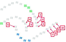
(a)

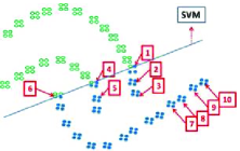
(b)

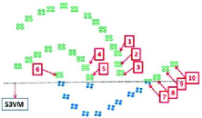
(c)

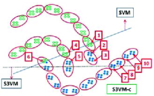
(d)

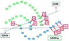
(e)

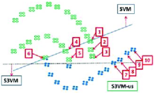
(f)

Figure 1: Illustration with artificial three-moon data. (a) Labeled data (empty and filled circles) and unlabeled data (gray points). The blocked numbers highlight groups of four unlabeled instances. Classification results of (b) Inductive SVM (using labeled data only); (c) S3VM; (d) S3VM-c, where each circle presents a cluster; (e) S3VM-p; (f) Our proposed S3VM-us.

Algorithm 1   S3VM-c

Input: $y_{SVM}$, $y_{S3VM}$, ${\cal D}$ and parameter $k$

1:  Perform partitional clustering (e.g., $k$means) on ${\cal D}$. Denote ${\cal C}_{1},\ldots,{\cal C}_{k}$ as the data indices of each cluster respectively.

2:  For each cluster $i=1,\ldots,k$, calculate the label bias $lb$ and confidence $cf$ of SVM and S3VM according to:

$$\small lb^{i}_{S(3)VM} = sign\left(\sum_{j\in{\cal C}_{i}}y_{S(3)VM}\left({\bf x}_{j}\right)\right)$$

$$cf^{i}_{S(3)VM} = \left|\sum_{j\in{\cal C}_{i}}y_{S(3)VM}\left({\bf x}_{j}\right)\right|.$$

3:  If $lb^{i}_{SVM}=lb^{i}_{S3VM}\;\;\&\;\;cf^{i}_{S3VM}>cf^{i}_{SVM}$, use the prediction of S3VM; otherwise use the prediction of SVM.

3.2 S3VM-p

The second baseline approach is motivated by confidence estimation in graph-based methods, e.g., zhu2003 , where the confidence can be naturally regarded as a risk measurement of unlabeled data.

Formally, to estimate the confidence of unlabeled data, let ${\bf F}^{l}=[({\bf y}_{l}+1)/2,(1-{\bf y}_{l})/2]\in\{0,1\}^{l\times 2}$ be the label matrix for labeled data where ${\bf y}_{l}=[y_{1},\ldots,y_{l}]^{\prime}\in\{\pm 1\}^{l\times 1}$ is the label vector. Let ${\bf W}=[w_{ij}]\in\mathcal{R}^{(l+u)\times(l+u)}$ be the weight matrix of training data and $\Lambda$ is the laplacian of ${\bf W}$, i.e., $\mbox{{\boldmath$\Lambda$}}={\bf D}-{\bf W}$ where ${\bf D}=diag(d_{i})$ is a diagonal matrix with entries $d_{i}=\sum_{j}w_{ij}$. Then, the predictions of unlabeled data can be obtained by zhu2003

$${\bf F}^{u}=\mbox{{\boldmath$\Lambda$}}_{u,u}^{-1}{\bf W}_{u,l}{\bf F}^{l},$$ (1)

where $\mbox{{\boldmath$\Lambda$}}_{u,u}$ is the sub-matrix of $\Lambda$ with respect to the block of unlabeled data, while ${\bf W}_{u,l}$ is the sub-matrix of ${\bf W}$ with respect to the block between labeled and unlabeled data. Then, assign each point ${\bf x}_{i}$ with the label $y_{LabPo}({\bf x}_{i})=\textrm{sgn}({\bf F}^{u}_{i-l,1}-{\bf F}^{u}_{i-l,2})$ and the confidence $h_{i}=|{\bf F}^{u}_{i-l,1}-{\bf F}^{u}_{i-l,2}|$. After confidence estimation, similar to S3VM-c, we consider the risk of unlabeled data by two factors, i.e., bias and confidence. If S3VM obtains the same bias of label propagation and the confidence is high enough, we use the S3VM prediction, and otherwise we take SVM prediction.

Algorithm 2 gives the S3VM-p method and Figure 1(e) illustrates the intuition of S3VM-p. As can be seen, the correct predictions of S3VM on groups $\{2,3\}$ are inherited by S3VM-p, while the wrong predictions of S3VM on groups $\{7,8,9,10\}$ are avoided.

Algorithm 2   S3VM-p

Input: $y_{SVM}$, $y_{S3VM}$, ${\cal D}$, ${\bf W}$ and parameter $\eta$

1:  Perform label propagation (e.g., zhu2003 ) with ${\bf W}$, obtain the predicted label $y_{lp}({\bf x}_{i})$ and confidence $h_{i}$ for each unlabeled instance ${\bf x}_{i}$, $i=l+1,\ldots,l+u$.

2:  Update ${\bf h}$ according to

$$h_{i}=y_{S3VM}({\bf x}_{i})y_{lp}({\bf x}_{i})h_{i},i=l+1,\ldots,l+u.$$

Let $c$ denote the number of nonnegative entries in ${\bf h}$.

3:  Sort ${\bf h}$, pick up the top-$\min\{\eta u,c\}$ values and use the predictions of S3VM for the corresponding unlabeled instances, otherwise use the predictions of SVM.

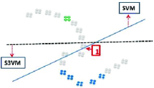
(a)

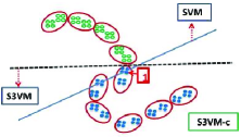
(b)

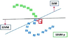
(c)

(d)

Figure 2: Illustration with artificial two-moon data when S3VM degenerates performance. (a) Labeled data (empty and filled circles) and unlabeled data (gray points). The blocked number highlight a group of four unlabeled instances. Classification results of (b) S3VM-c, where each circle presents a cluster; (c) S3VM-p; (d) Our proposed S3VM-us.

4 Our Proposed Method

4.1 Deficiencies of S3VM-c and S3VM-p

S3VM-c and S3VM-p are capable of reducing the chances of performance degeneration by using unlabeled data, however, they both suffer from some deficiencies. For S3VM-c, it works in a local manner and the relation between clusters are never considered, leading to the unexploitation of some helpful unlabeled instances, e.g., unlabeled instances in groups $\{2,3\}$ in Figure 2(d). For S3VM-p, as stated in wang2008graph , the confidence estimated by label propagation approach might be incorrect if the label initialization is highly imbalanced, leading to the unexploitation of some useful unlabeled instances, e.g., groups $\{4,5\}$ in Figure 2(e).

Moreover, both S3VM-c and S3VM-p heavily rely on the predictions of S3VM, which might become a serious issue especially when S3VM obtains degenerated performance. Figures 2(b) and 2(c) illustrate the behaviors of S3VM-c and S3VM-p when S3VM degenerates performance. Both S3VM-c and S3VM-p erroneously inherit the wrong predictions of S3VM of group 1.

4.2 S3VM-us

The deficiencies of S3VM-c and S3VM-p suggest to take into account of cluster relation and make the method insensitive to label initialization. This motivates us to use hierarchical clustering jain1988algorithms , leading to our proposed method S3VM-us.

Hierarchical clustering works in a greedy and iterative manner. It first initials each singe instance as a cluster and then at each step, it merges two clusters with the shortest distance among all pairs of clusters. In this step, the cluster relation is considered and moreover, since hierarchical clustering works in an unsupervised setting, it does not suffer from the label initialization problem.

Suppose $p_{i}$ and $n_{i}$ are the lengths of paths from the instance ${\bf x}_{i}$ to its nearest positive and negative labeled instances, respectively, in hierarchical clustering. We simply take the difference between $p_{i}$ and $n_{i}$ as an estimation of the confidence on the unlabeled instance ${\bf x}_{i}$. Intuitively, the larger the difference between $p_{i}$ and $n_{i}$, the higher the confidence on labeling ${\bf x}_{i}$.

Algorithm 3 gives the S3VM-us method and Figures 1(f) and 2 illustrate the intuition of S3VM-us. As can be seen, the wrong predictions of S3VM on groups $\{7,8,9,10\}$ are avoided by S3VM-us, the correct predictions of S3VM on groups $\{2,3,4,5\}$ are inherited, and S3VM-us does not erroneously inherit the wrong predictions of S3VM on group 1 in Figure 2.

Algorithm 3   S3VM-us

Input: $y_{SVM}$, $y_{S3VM}$, ${\cal D}$ and parameter $\epsilon$

1:  Let $\mathcal{S}$ be a set of the unlabeled data ${\bf x}$ such that $y_{SVM}({\bf x})\neq y_{S3VM}({\bf x})$.

2:  Perform hierarchical clustering, e.g., single linkage method jain1988algorithms .

3:  For each unlabeled instance ${\bf x}_{i}\in\mathcal{S}$, calculate $p_{i}$ and $n_{i}$, that is, the length of the paths from ${\bf x}_{i}$ to its nearest positive and negative labeled instances, respectively. Denote $t_{i}=(n_{i}-p_{i})$.

4:  Let $\mathcal{B}$ be the set of unlabeled instances ${\bf x}_{i}$ in $\mathcal{S}$ satisfying $|t_{i}|\geq\epsilon|l+u|$.

5:  If $\sum_{{\bf x}_{i}\in\mathcal{B}}y_{S3VM}({\bf x}_{i})t_{i}\geq\sum_{{\bf x}_{i}\in\mathcal{B}}y_{SVM}({\bf x}_{i})t_{i}$, predict the unlabeled instances in $\mathcal{B}$ by S3VM and otherwise by SVM.

6:  Predict the unlabeled data ${\bf x}\not\in\mathcal{B}$ by SVM.

5 Experiments

5.1 Settings

We evaluate S3VM-us on a broad range of data sets including the semi-supervised learning benchmark data sets in chapelle2006ssl and sixteen UCI data sets. The benchmark data sets are g241c, g241d, Digit1, USPS, TEXT and BCI. For each data, the archive provides two data sets with one using 10 labeled examples and the other using 100 labeled examples. As for UCI data sets, we randomly select 10 and 100 examples to be used as labeled examples, respectively, and use the remaining data as unlabeled data. The experiments are repeated for 30 times and the average accuracies and standard deviations are recorded. It is worth noting that in semi-supervised learning, labeled examples are often too few to afford a valid cross validation, and therefore hold-out tests are usually used for the evaluation.

In addition to S3VM-c and S3VM-p, we compare with inductive SVM and TSVM Joachims1999 . Both linear and Gaussian kernels are used. For the benchmark data sets, we follow the setup in chapelle2006ssl . Specifically, for the case of 10 labeled examples, the parameter $C$ for SVM is fixed to $m/\sum_{i=1}^{m}{\|{\bf x}_{i}\|^{2}}$ where $m=l+u$ is the size of data set and the Gaussian kernel width is set to $\delta$, i.e., the average distance between instances. For the case of $100$ labeled examples, $C$ is fixed to 100 and the Gaussian kernel width is selected from $\{0.25\delta,0.5\delta,\delta,2\delta,4\delta\}$ by cross validation. On UCI data sets, the parameter $C$ is fixed to 1 and the Gaussian kernel width is set to $\delta$ for 10 labeled examples. For 100 label examples, the parameter $C$ is selected from $\{0.1,1,10,100\}$ and the Gaussian kernel width is selected from $\{0.25\delta,0.5\delta,\delta,2\delta,4\delta\}$ by cross validation. For S3VM-c, the cluster number $k$ is fixed to 50; for S3VM-p, the weighted matrix is constructed via Gaussian distance and the parameter $\eta$ is fixed to 0.1; for S3VM-us, the parameter $\epsilon$ is fixed to 0.1.

5.2 Results

Table 1: Accuracy (mean $\pm$ std.) on 10 labeled examples. ‘SVM’ denotes inductive SVM which uses labeled data only. For the semi-supervised methods (TSVM, S3VM-c, S3VM-p and S3VM-us), if the performance is significantly better/worse than SVM, the corresponding entries are bolded/underlined (paired $t$-tests at 95% significance level). The win/tie/loss counts with the fewest losses are bolded.

Data	SVM	TSVM	S3VM-c	S3VM-p	S3VM-us
	( linear / gaussian )	( linear / gaussian )	( linear / gaussian )	( linear / gaussian )	( linear / gaussian )
BCI	50.7$\pm$1.5 / 52.7$\pm$2.7	49.3$\pm$2.8 / 51.4$\pm$2.7	50.2$\pm$2.0 / 52.2$\pm$2.6	50.6$\pm$1.6 / 52.6$\pm$2.7	50.9$\pm$1.6 / 52.6$\pm$2.7
g241c	53.2$\pm$4.8 / 53.0$\pm$4.5	78.9$\pm$4.7 / 78.5$\pm$5.0	55.2$\pm$8.3 / 55.3$\pm$8.8	53.9$\pm$5.8 / 53.6$\pm$5.3	53.5$\pm$4.8 / 53.2$\pm$4.5
g241d	54.4$\pm$5.4 / 54.5$\pm$5.2	53.6$\pm$7.8 / 53.2$\pm$6.5	53.8$\pm$5.4 / 53.6$\pm$5.0	54.1$\pm$5.3 / 54.0$\pm$5.2	54.4$\pm$5.3 / 54.4$\pm$5.2
digit1	55.4$\pm$10.9 / 75.0$\pm$7.9	79.4$\pm$1.1 / 81.5$\pm$3.1	56.1$\pm$12.2 / 77.3$\pm$8.2	56.2$\pm$12.2 / 75.0$\pm$8.1	58.1$\pm$9.6 / 75.1$\pm$7.8
USPS	80.0$\pm$0.1 / 80.7$\pm$1.8	69.4$\pm$1.2 / 73.0$\pm$2.6	80.0$\pm$0.1 / 80.4$\pm$2.5	80.0$\pm$0.1 / 80.5$\pm$2.1	80.0$\pm$0.1 / 80.7$\pm$1.8
Text	54.7$\pm$6.3 / 54.6$\pm$6.3	71.4$\pm$11.7 / 71.2$\pm$11.4	56.8$\pm$8.8 / 56.5$\pm$8.7	55.3$\pm$6.6 / 55.2$\pm$6.8	58.0$\pm$9.0 / 57.8$\pm$8.9
house	90.0$\pm$6.0 / 84.8$\pm$11.8	84.6$\pm$8.0 / 84.7$\pm$6.9	89.8$\pm$6.2 / 84.8$\pm$11.9	89.5$\pm$6.0 / 84.5$\pm$11.8	90.1$\pm$6.1 / 85.4$\pm$11.4
heart	58.8$\pm$10.5 / 63.9$\pm$11.6	72.4$\pm$12.6 / 72.6$\pm$10.4	59.0$\pm$10.8 / 64.4$\pm$11.6	58.6$\pm$10.6 / 63.8$\pm$11.7	61.9$\pm$9.7 / 65.1$\pm$11.0
heart-statlog	74.6$\pm$4.8 / 69.9$\pm$10.1	74.9$\pm$6.6 / 73.9$\pm$5.9	74.5$\pm$5.2 / 70.1$\pm$10.2	74.5$\pm$4.9 / 70.0$\pm$10.2	74.2$\pm$5.4 / 71.7$\pm$6.9
ionosphere	70.4$\pm$8.7 / 65.8$\pm$9.8	72.0$\pm$10.5 / 76.1$\pm$8.2	70.9$\pm$9.0 / 66.1$\pm$9.9	70.4$\pm$8.7 / 66.0$\pm$9.7	70.7$\pm$8.3 / 67.4$\pm$6.7
vehicle	73.2$\pm$8.9 / 58.3$\pm$9.5	72.1$\pm$9.4 / 63.2$\pm$7.8	73.5$\pm$9.4 / 58.4$\pm$9.6	72.6$\pm$9.1 / 58.0$\pm$9.5	74.5$\pm$9.3 / 64.2$\pm$9.1
house-votes	85.5$\pm$7.0 / 79.7$\pm$10.7	83.8$\pm$6.1 / 84.0$\pm$5.3	85.7$\pm$7.0 / 80.1$\pm$10.6	85.3$\pm$6.9 / 79.7$\pm$10.7	86.0$\pm$5.7 / 84.3$\pm$6.1
wdbc	65.6$\pm$7.5 / 73.8$\pm$10.3	90.0$\pm$6.1 / 88.9$\pm$3.7	65.7$\pm$7.8 / 74.9$\pm$10.9	66.1$\pm$8.0 / 73.9$\pm$10.5	65.8$\pm$7.5 / 73.9$\pm$10.3
clean1	58.2$\pm$4.2 / 53.5$\pm$6.2	57.0$\pm$5.1 / 53.3$\pm$4.8	57.8$\pm$4.4 / 53.3$\pm$6.2	58.5$\pm$4.2 / 53.3$\pm$6.3	58.2$\pm$4.2 / 55.0$\pm$8.1
isolet	93.8$\pm$4.3 / 82.0$\pm$15.7	84.2$\pm$10.9 / 86.7$\pm$9.5	94.5$\pm$5.1 / 83.2$\pm$16.0	93.0$\pm$4.7 / 81.7$\pm$15.7	93.7$\pm$4.3 / 84.1$\pm$12.6
breastw	93.9$\pm$4.8 / 92.3$\pm$10.1	89.2$\pm$8.6 / 88.9$\pm$8.8	94.2$\pm$4.9 / 92.4$\pm$10.0	93.9$\pm$4.9 / 92.2$\pm$10.0	93.6$\pm$5.4 / 92.4$\pm$9.9
australian	70.4$\pm$9.2 / 60.3$\pm$8.4	69.6$\pm$11.9 / 68.6$\pm$11.4	70.1$\pm$9.8 / 60.4$\pm$8.3	70.5$\pm$9.4 / 60.5$\pm$8.8	70.3$\pm$9.2 / 60.8$\pm$7.9
diabetes	63.3$\pm$6.9 / 66.3$\pm$3.5	63.4$\pm$7.6 / 65.8$\pm$4.6	63.2$\pm$6.8 / 65.9$\pm$3.0	63.4$\pm$6.6 / 66.2$\pm$3.4	63.3$\pm$6.9 / 66.3$\pm$3.5
german	65.2$\pm$4.9 / 65.1$\pm$12.0	63.7$\pm$5.6 / 63.5$\pm$5.1	65.6$\pm$4.7 / 65.1$\pm$11.8	65.6$\pm$4.8 / 65.1$\pm$11.9	65.2$\pm$5.0 / 65.3$\pm$11.6
optdigits	96.1$\pm$3.2 / 92.8$\pm$9.6	89.8$\pm$9.2 / 91.4$\pm$7.6	96.6$\pm$3.1 / 93.6$\pm$9.9	95.6$\pm$3.0 / 92.4$\pm$9.8	96.9$\pm$2.5 / 94.9$\pm$5.8
ethn	56.5$\pm$8.8 / 58.5$\pm$10.2	64.2$\pm$13.5 / 68.1$\pm$14.5	56.5$\pm$8.6 / 59.4$\pm$11.6	56.8$\pm$9.1 / 58.6$\pm$10.7	59.8$\pm$10.7 / 61.8$\pm$11.3
sat	95.8$\pm$4.1 / 87.5$\pm$10.9	85.5$\pm$11.4 / 86.5$\pm$10.8	96.3$\pm$4.1 / 87.7$\pm$11.2	94.8$\pm$4.2 / 86.9$\pm$10.8	96.4$\pm$3.9 / 90.7$\pm$8.1
Aver. Acc.	70.9 / 69.3	73.5 / 73.8	71.2 / 69.8	70.9 / 69.3	71.6 / 70.8
SVM vs. Semi-Supervised: W/T/L		18/18/8	14/29/1	7/25/12	12/32/0

Table 2: Accuracy (mean $\pm$ std.) on 100 labeled examples. ‘SVM’ denotes inductive SVM which uses labeled data only. For the semi-supervised methods (TSVM, S3VM-c, S3VM-p and S3VM-us), if the performance is significantly better/worse than SVM, the corresponding entries are bolded/underlined (paired $t$-tests at 95% significance level). The win/tie/loss counts with the fewest losses are bolded.

Data	SVM	TSVM	S3VM-c	S3VM-p	S3VM-us
	( linear / gaussian )	( linear / gaussian )	( linear / gaussian )	( linear / gaussian )	( linear / gaussian )
BCI	61.1$\pm$2.6 / 65.9$\pm$3.1	56.4$\pm$2.8 / 65.6$\pm$2.5	58.3$\pm$2.6 / 65.6$\pm$3.0	60.3$\pm$2.5 / 65.8$\pm$3.0	61.0$\pm$2.7 / 65.8$\pm$3.1
g241c	76.3$\pm$2.0 / 76.6$\pm$2.1	81.7$\pm$1.6 / 82.1$\pm$1.2	79.3$\pm$1.7 / 79.6$\pm$1.8	77.2$\pm$2.1 / 77.1$\pm$2.0	76.3$\pm$2.0 / 76.6$\pm$2.1
g241d	74.2$\pm$1.9 / 75.4$\pm$1.8	76.1$\pm$8.5 / 77.9$\pm$7.4	77.4$\pm$3.5 / 78.5$\pm$3.3	74.8$\pm$2.3 / 75.7$\pm$2.2	74.2$\pm$1.9 / 75.4$\pm$1.8
digit1	50.3$\pm$1.2 / 94.0$\pm$1.4	81.9$\pm$3.0 / 94.0$\pm$2.0	50.3$\pm$1.2 / 95.0$\pm$1.5	50.3$\pm$1.2 / 94.1$\pm$1.4	67.9$\pm$1.3 / 94.1$\pm$1.4
USPS	80.0$\pm$0.2 / 91.7$\pm$1.1	78.8$\pm$2.0 / 90.9$\pm$1.4	80.0$\pm$0.2 / 92.5$\pm$1.0	80.0$\pm$0.2 / 91.6$\pm$1.2	80.1$\pm$0.4 / 91.8$\pm$1.1
Text	73.8$\pm$3.3 / 73.7$\pm$3.6	77.7$\pm$1.6 / 77.7$\pm$1.7	75.3$\pm$3.4 / 75.2$\pm$3.6	73.9$\pm$3.4 / 73.8$\pm$3.7	74.1$\pm$3.1 / 74.2$\pm$3.3
house	95.7$\pm$2.0 / 95.6$\pm$1.6	94.4$\pm$2.5 / 94.8$\pm$2.6	95.5$\pm$1.8 / 95.4$\pm$1.8	95.6$\pm$2.0 / 95.5$\pm$1.7	95.6$\pm$2.0 / 95.6$\pm$1.6
heart	81.5$\pm$2.5 / 80.1$\pm$2.4	80.7$\pm$3.1 / 79.5$\pm$2.9	81.1$\pm$3.0 / 79.8$\pm$2.5	81.5$\pm$2.5 / 80.2$\pm$2.5	81.5$\pm$2.6 / 80.1$\pm$2.4
heart-statlog	81.5$\pm$2.4 / 81.4$\pm$2.7	81.6$\pm$2.7 / 79.0$\pm$4.5	81.2$\pm$2.2 / 80.7$\pm$3.0	81.5$\pm$2.4 / 81.2$\pm$2.7	81.5$\pm$2.4 / 81.3$\pm$2.7
ionosphere	87.1$\pm$1.5 / 93.2$\pm$1.6	85.6$\pm$2.1 / 92.1$\pm$2.3	88.7$\pm$1.3 / 93.4$\pm$1.5	87.1$\pm$1.5 / 93.2$\pm$1.6	87.1$\pm$1.5 / 93.2$\pm$1.6
vehicle	92.9$\pm$1.7 / 95.4$\pm$1.4	91.6$\pm$2.5 / 95.4$\pm$2.3	93.3$\pm$1.6 / 95.9$\pm$1.3	92.8$\pm$1.7 / 95.2$\pm$1.5	93.0$\pm$1.7 / 95.5$\pm$1.4
house-votes	92.3$\pm$1.3 / 92.8$\pm$1.2	92.0$\pm$1.8 / 93.0$\pm$1.4	92.6$\pm$1.2 / 92.9$\pm$1.2	92.3$\pm$1.3 / 92.8$\pm$1.2	92.3$\pm$1.3 / 92.8$\pm$1.2
clean1	73.0$\pm$2.7 / 80.6$\pm$3.0	73.2$\pm$3.1 / 79.1$\pm$3.4	73.7$\pm$2.9 / 79.9$\pm$2.9	73.2$\pm$2.6 / 80.4$\pm$3.2	73.1$\pm$2.7 / 80.7$\pm$3.0
wdbc	95.6$\pm$0.8 / 94.7$\pm$0.9	94.3$\pm$2.3 / 94.1$\pm$2.4	95.8$\pm$0.7 / 94.9$\pm$0.9	95.6$\pm$0.8 / 94.7$\pm$0.9	95.6$\pm$0.8 / 94.8$\pm$0.9
isolet	99.2$\pm$0.4 / 99.0$\pm$0.6	95.9$\pm$3.1 / 98.2$\pm$2.3	99.2$\pm$0.4 / 99.2$\pm$0.5	99.0$\pm$0.4 / 98.9$\pm$0.6	99.2$\pm$0.4 / 99.1$\pm$0.5
breastw	96.4$\pm$0.4 / 96.7$\pm$0.4	96.9$\pm$1.9 / 97.1$\pm$0.5	96.6$\pm$0.4 / 96.9$\pm$0.4	96.3$\pm$0.4 / 96.7$\pm$0.4	96.4$\pm$0.4 / 96.7$\pm$0.4
australian	83.8$\pm$1.6 / 84.9$\pm$1.7	82.5$\pm$2.6 / 84.6$\pm$2.7	83.8$\pm$1.7 / 85.0$\pm$1.6	83.9$\pm$1.7 / 85.0$\pm$1.8	83.8$\pm$1.7 / 85.0$\pm$1.7
diabetes	75.2$\pm$1.7 / 74.7$\pm$1.9	72.3$\pm$2.3 / 71.8$\pm$1.8	74.9$\pm$1.7 / 74.2$\pm$2.2	75.3$\pm$1.6 / 74.7$\pm$1.9	75.2$\pm$1.8 / 74.7$\pm$1.9
german	67.1$\pm$2.4 / 72.0$\pm$1.5	66.1$\pm$2.1 / 65.9$\pm$3.4	67.1$\pm$2.2 / 71.6$\pm$1.5	67.6$\pm$2.3 / 72.1$\pm$1.4	67.1$\pm$2.4 / 72.1$\pm$1.5
optdigits	99.4$\pm$0.3 / 99.4$\pm$0.3	95.9$\pm$3.7 / 97.4$\pm$3.1	99.5$\pm$0.4 / 99.5$\pm$0.3	99.2$\pm$0.4 / 99.2$\pm$0.4	99.5$\pm$0.3 / 99.4$\pm$0.3
ethn	91.6$\pm$1.6 / 93.4$\pm$1.2	92.6$\pm$2.3 / 93.4$\pm$3.0	93.9$\pm$1.6 / 95.0$\pm$1.2	91.9$\pm$1.5 / 93.3$\pm$1.2	91.7$\pm$1.5 / 93.4$\pm$1.2
sat	99.7$\pm$0.2 / 99.7$\pm$0.1	96.4$\pm$2.8 / 97.6$\pm$2.7	99.7$\pm$0.2 / 99.8$\pm$0.1	99.5$\pm$0.3 / 99.5$\pm$0.3	99.7$\pm$0.2 / 99.7$\pm$0.1
Aver. Acc.	83.0 / 86.8	83.9 / 86.4	83.5 / 87.3	83.1 / 86.8	83.9 / 86.9
SVM vs. Semi-Supervised: W/T/L		7/18/19	21/16/7	8/25/11	8/36/0

The results are shown in Tables 1 and 2. As can be seen, the performance of S3VM-us is competitive with TSVM. In terms of average accuracy, TSVM performs slightly better (worse) than S3VM-us on the case of 10 (100) labeled examples. In terms of pairwise comparison, S3VM-us performs better than TSVM on 13/12 and 14/16 cases with linear/Gaussian kernel for 10 and 100 labeled examples, respectively. Note that in a number of cases, TSVM has large performance improvement against inductive SVM, while the improvement of S3VM-us is smaller. This is not a surprise since S3VM-us tries to improve performance with the caution of avoiding performance degeneration.

Though TSVM has large improvement in a number of cases, it also has large performance degeneration in cases. Indeed, as can be seen from Tables 1 and 2, TSVM is significantly inferior to inductive SVM on 8/44, 19/44 cases for 10 and 100 labeled examples, respectively. Both S3VM-c and S3VM-p are capable to reduce the times of significant performance degeneration, while S3VM-us does not significantly degenerate performance in the experiments.

5.3 Parameter Influence

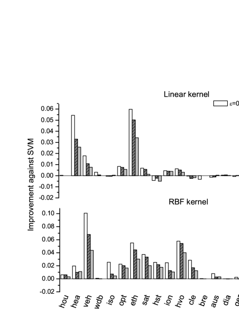
Figure 3: Influence of the parameter $\epsilon$ on the improvement of S3VM-us against inductive SVM.

S3VM-us has a parameter $\epsilon$. To study the influence of $\epsilon$, we run experiments by setting $\epsilon$ to different values (0.1, 0.2 and 0.3) with 10 labeled examples. The results are plotted in Figure 3. It can be seen that the setting of $\epsilon$ has influence on the improvement of S3VM-us against inductive SVM. Whatever linear kernel or gaussian kernel is used, the larger the value of $\epsilon$, the closer the performance of S3VM-us to SVM. It may be possible to increase the performance improvement by setting a smaller $\epsilon$, however, this may increase the risk of performance degeneration.

6 Conclusion

In this paper we propose the S3VM-us method. Rather than simply predicting all unlabeled instances by semi-supervised learner, S3VM-us uses hierarchical clustering to help select unlabeled instances to be predicted by semi-supervised learner and predict the remaining unlabeled instances by inductive learner. In this way, the risk of performance degeneration by using unlabeled data is reduced. The effectiveness of S3VM-us is validated by empirical study.

The proposal in this paper is based on heuristics and theoretical analysis is future work. It is worth noting that, along with reducing the chance of performance degeneration, S3VM-us also reduces the possible performance gains from unlabeled data. In the future it is desirable to develop really safe semi-supervised learning approaches which are able to improve performance significantly but never degenerate performance by using unlabeled data.

References

- [1] M. F. Balcan, A. Blum, P. P. Choi, J. Lafferty, B. Pantano, M. R. Rwebangira, and X. Zhu. Person identification in webcam images: An application of semi-supervised learning. In ICML Workshop on Learning with Partially Classified Training Data, 2005.
- [2] S. Ben-David, T. Lu, and D. Pál. Does unlabeled data provably help? Worst-case analysis of the sample complexity of semi-supervised learning. In COLT, pages 33–44, 2008.
- [3] K. Bennett and A. Demiriz. Semi-supervised support vector machines. In NIPS 11, pages 368–374. 1999.
- [4] A. Blum and S. Chawla. Learning from labeled and unlabeled data using graph mincuts. In ICML, pages 19–26, 2001.
- [5] A. Blum and T. Mitchell. Combining labeled and unlabeled data with co-training. In COLT, pages 92–100, 1998.
- [6] O. Chapelle, B. Schölkopf, and A. Zien, editors. Semi-Supervised Learning. MIT Press, Cambridge, MA, 2006.
- [7] O. Chapelle, V. Sindhwani, and S. S. Keerthi. Optimization techniques for semi-supervised support vector machines. J. Mach. Learn. Res., 9:203–233, 2008.
- [8] O. Chapelle and A. Zien. Semi-supervised learning by low density separation. In AISTATS, pages 57–64, 2005.
- [9] N. V. Chawla and G. Karakoulas. Learning from labeled and unlabeled data: An empirical study across techniques and domains. J. Artif. Intell. Res., 23:331–366, 2005.
- [10] R. Collobert, F. Sinz, J. Weston, and L. Bottou. Large scale transductive SVMs. J. Mach. Learn. Res., 7:1687–1712, 2006.
- [11] F. G. Cozman, I. Cohen, and M. C. Cirelo. Semi-supervised learning of mixture models. In ICML, pages 99–106, 2003.
- [12] S. Dasgupta, M. L. Littman, and D. McAllester. PAC generalization bounds for co-training. In NIPS 14, pages 375–382. 2002.
- [13] A.K. Jain and R.C. Dubes. Algorithms for Clustering Data. Prentice Hall, Englewood Cliffs, NJ., 1988.
- [14] T. Jebara, J. Wang, and S. F. Chang. Graph construction and b-matching for semi-supervised learning. In ICML, pages 441–448, 2009.
- [15] T. Joachims. Transductive inference for text classification using support vector machines. In ICML, pages 200–209, 1999.
- [16] J. Lafferty and L. Wasserman. Statistical analysis of semi-supervised regression. In NIPS 20, pages 801–808. 2008.
- [17] M. Li and Z. H. Zhou. SETRED: Self-training with editing. In PAKDD, pages 611–621, 2005.
- [18] Y.-F. Li, J. T. Kwok, and Z.-H. Zhou. Semi-supervised learning using label mean. In ICML, pages 633–640, 2009.
- [19] D. J. Miller and H. S. Uyar. A mixture of experts classifier with learning based on both labelled and unlabelled data. In NIPS 9, pages 571–577. 1997.
- [20] K. Nigam, A. K. McCallum, S. Thrun, and T. Mitchell. Text classification from labeled and unlabeled documents using EM. Mach. Learn., 39(2):103–134, 2000.
- [21] A. Singh, R. Nowak, and X. Zhu. Unlabeled data: Now it helps, now it doesn’t. In NIPS 21, pages 1513–1520. 2009.
- [22] J. Wang, T. Jebara, and S. F. Chang. Graph transduction via alternating minimization. In ICML, pages 1144–1151, 2008.
- [23] W. Wang and Z.-H. Zhou. Analyzing co-training style algorithms. In ECML, pages 454–465, 2007.
- [24] W. Wang and Z.-H. Zhou. A new analysis of co-training. In ICML, pages 1135–1142, 2010.
- [25] T. Zhang and F. Oles. The value of unlabeled data for classification problems. In ICML, pages 1191–1198, 2000.
- [26] D. Zhou, O. Bousquet, T. N. Lal, J. Weston, and B. Scholkopf. Learning with local and global consistency. In NIPS 16, pages 595–602. 2004.
- [27] Z.-H. Zhou and M. Li. Tri-training: Exploiting unlabeled data using three classifiers. IEEE Trans. Knowl. Data Eng., 17(11):1529–1541, 2005.
- [28] Z.-H. Zhou and M. Li. Semi-supervised learning by disagreement. Knowl. Inf. Syst., 24(3):415–439, 2010.
- [29] X. Zhu. Semi-supervised learning literature survey. Technical Report 1530, Dept. Comp. Sci., Univ. Wisconsin-Madison, 2006.
- [30] X. Zhu, Z. Ghahramani, and J. D. Lafferty. Semi-supervised learning using gaussian fields and harmonic functions. In ICML, pages 912–919, 2003.