Direct and inverse cascades in geodynmo

Zusammenfassung

The rapid rotation of the planets causes cyclonic thermal turbulence in the cores, which can be responsible for the generation of the large-scale magnetic fields observed out of the planets. We consider the model which lets us to reproduce the typical features of the small-scale geostrophic flows in the physical and wave spaces. We present estimates of kinetic and magnetic energies fluxes as a function of the wave number. The joined existence of the forward and inverse cascades are demonstrated. We also consider mechanism of the magnetic field saturation at the end of the kinematic dynamo regime.

Many astrophysical objects such as galaxies, stars, the earth, and some of the planets have large scale magnetic fields that are believed to be generated by a common universal mechanism - the conversion of kinetic energy into magnetic energy in a turbulent rotating shell. The details, however, - and thus the nature of the resulting field - differ greatly. The challenge for the dynamo theory see, e.g., (Hollerbach and R$\ddot{\rm u}$diger, 2004), is to provide a model that can explain the visible features of the field with realistic assumptions on the model parameters. Calculations for the entire planet are done either with spectral models (Kono and Roberts, 2002) or finite volume methods (Hejda and Reshetnyak, 2004; Harden and Hansen, 2005) and finite difference (Kageyama and Sato, 1997), and have demonstrated beyond reasonable doubt that the turbulent 3D convection of the conductive fluid can generate a large scale magnetic field similar to the one observed out of small random fluctuations. However, both these methods cannot cover the enormous span of scales required for a realistic parameter set. Even for the geodynamo (which is quite a modest on astrophysical scales case) the hydrodynamic Reynolds number estimated on the west drift velocity is $\mathop{\rm Re}\nolimits\sim 10^{9}$. In addition planets are the rapidly rotating bodies. So, the time scale of the large-scale convection in the Earth’s core is $\sim 10^{3}$ years, during which the planet itself makes $\sim 10^{6}$ revolutions (in other words the Rossby number $\mathop{\rm Ro}\nolimits\sim 10^{-6}$). As a result, there is an additional spatial scale $\sim\mathop{\rm E}\nolimits^{-1/3}L$, where $\mathop{\rm E}\nolimits\sim 10^{-15}$ is the Ekman number (Chandrasekhar, 1961; Busse, 1970), associated with the cyclonic structures elongated along axis of rotation, which is quite larger then the Kolmogorov’s dissipation scale $l_{d}\sim\mathop{\rm Re}\nolimits^{-4/3}{L}$ however which is still too small to be resolved in the numerical simulations with present resolution $l\sim(10^{-3}\div 10^{-2}){L}$ with $L$ for the large scale.

Presence of the rapid rotation leads not only to the change of the spatial uniform isotropic Kolmogorov like solution to the quasi-geostrophic (magnetostrophic) form but to rather more fundamental consequences. Rapid rotation leads to degeneration of the third dimension (along the axis of rotation) and can cause inverse cascade in the system. The inverse cascades is a well-known phenomenon in the two-dimensional turbulence and is a good example of self-organization, when the large-scale structures are feeded by the small-scales turbulence (Kraichnan and Montgomery, 1980; Tabeling, 2002). So far, that the quasi-geostrophic state formally still is a three dimensional (the vector fields have three components) behavior of such systems can differ from the two-dimensional flows as well as from the three dimensional ones. It can happen, that quasi-geostrophic turbulence can exhibit simultaneously features similar to the both extreme cases: 2D and 3D. Further we consider behavior of the fluxes of the energy in the wave space for the well-known in geodynamo regimes based on the Boussinesque thermal convection. For simplicity we consider the Cartesian geometry which is simpler for modeling of the rapidly rotating dynamo systems and was used in many researches on geodynamo Roberts (1999); Jones and Roberts (2000); Buffett (2003).

1 Dynamo equtions

1.1 Equations in physical space

The geodynamo equations for the incompressible fluid ($\nabla\cdot{\bf V}=0$) in the volume of the scale $L$ rotating with the angular velocity $\Omega$ in the Cartesian system of coordinates $(x,\,y,\,z)$ in its traditional dimensionless form can be written as follows:

$$\begin{array}[]{l}\displaystyle\frac{{\partial}{\bf B}}{{\partial t}}={\nabla}\times\left({\bf V}\times{\bf B}\right)+\mathop{\rm q}\nolimits^{-1}\Delta{\bf B}\\ \displaystyle\mathop{\rm E}\nolimits\mathop{\rm Pr}\nolimits^{-1}\left[\frac{{\partial}{\bf V}}{\partial t}+\left({\bf V}\cdot\nabla\right){\bf V}\right]=-\nabla{P}-{\bf{1}_{z}}\times{\bf V}+\\ \qquad\qquad\mathop{\rm Ra}\nolimits{T}\,z{\bf{1}_{z}}+\left(\nabla\times{\bf B}\right)\times{\bf B}+\mathop{\rm E}\nolimits\Delta{\bf V}\\ \displaystyle\frac{\partial{T}}{\partial t}+\left({\bf V}\cdot\nabla\right)\left({T}+{T}_{0}\right)=\Delta{T}.\end{array}$$ (1)

The velocity $\bf V$, magnetic field $\bf B$, pressure $P$ and typical diffusion time $t$ are measured in units of $\kappa/L$, $\displaystyle\sqrt{2\Omega\kappa\mu\rho};$, $\rm\rho\kappa^{2}/L^{2}$ and $\rm L^{2}/\kappa$ respectively, where $\kappa$ is thermal diffusivity, $\rho$ is density, $\mu$ permeability, $\displaystyle\mathop{\rm Pr}\nolimits=\frac{\kappa}{\nu}$ is the Prandtl number, $\displaystyle\mathop{\rm E}\nolimits=\frac{\nu}{2\Omega L^{2}}$ is the Ekman number, $\nu$ is kinematic viscosity, $\eta$ is the magnetic diffusivity, and ${\mathop{\rm q}\nolimits}=\kappa/\eta$ is the Roberts number. $\displaystyle\mathop{\rm Ra}\nolimits=\frac{\alpha g_{0}\delta T{L}}{2\Omega\kappa}$ is the modified Rayleigh number, $\alpha$ is the coefficient of volume expansion, $\delta T$ is the unit of temperature, see for more details Jones (2000), $g_{0}$ is the gravitational acceleration, and $T_{0}=1-z$ is the heating below. The problem is closed with the periodical boundary conditions in the $(x,\,y)$ plane. In $z$-direction we use simplified conditions (Cattaneo et al, 2003): $T_{0}=0$, $\displaystyle V_{z}={\partial V_{x}\over\partial z}={\partial V_{y}\over\partial z}=0$, $\displaystyle B_{x}=B_{y}={\partial B_{z}\over\partial z}=0$ at $z=0,\,1$.

1.2 Equations in wave space

To solve the problem (1) we apply pseudo-spectral approach (Orszag, 1971) frequently used in geodynamo simulations (Jones and Roberts, 2000; Buffett, 2003). Equations are solved in the wave space. To calculate the non-linear terms one needs make the inverse Fourier transform, then calculate a product in the physical space, make a Fourier transform of the product, and finally calculate a derivatives in the wave space. After elimination of the pressure using conditions of the free divergency ${\bf k}\cdot{\bf V}=0$, ${\bf k}\cdot{\bf B}=0$ we come to

$$\begin{array}[]{l}\displaystyle\left[{{\partial}{\bf B}\over{\partial t}}+\mathop{\rm q}\nolimits^{-1}k^{2}{\bf B}\right]_{\bf k}=\left[{\nabla}\times\left({\bf V}\times{\bf B}\right)\right]_{\bf k}\\ \\ \displaystyle\mathop{\rm E}\nolimits\left[\mathop{\rm Pr}\nolimits^{-1}{\partial{\bf V}\over\partial t}+k^{2}{\bf V}\right]_{\bf k}={\bf k}{\cal P}_{\bf k}+{\bf F}_{\bf k}\\ \\ \displaystyle\left[{\partial{T}\over\partial t}+k^{2}T\right]_{\bf k}=-\left[\left({\bf V}\cdot\nabla\right){T}+V_{r}\right]_{\bf k}\end{array}$$ (2)

with

$$\begin{array}[]{l}\displaystyle\par{\cal P}_{\bf k}=-{{\bf k}\cdot{\bf F}_{\bf k}\over k^{2}},\qquad\displaystyle k^{2}=k_{\beta}k_{\beta},\qquad\beta=1\dots 3\\ \\ \displaystyle{\bf F}_{\bf k}=\Big{[}\mathop{\rm Pr}\nolimits^{-1}{\bf V}\times\left(\nabla\times{\bf V}\right)+\mathop{\rm Ra}\nolimits T{\bf{1}_{z}}-\\ \qquad{\bf 1_{z}}\times{\bf V}+\left({\bf B}\cdot\nabla\right){\bf B}\Big{]}_{\bf k}.\end{array}$$ (3)

For integration in time we use explicit Adams-Bashforth (AB2) scheme for the non-linear terms. The linear terms are treated using the Crank-Nicolson (CN) scheme. To resolve the diffusion terms we use the known trick which helps to increase the time step significantly. Consider equation

$$\begin{array}[]{l}\displaystyle{\partial A\over\partial t}+k^{2}A=U\end{array}$$ (4)

rewrite it in the form

$$\begin{array}[]{l}\displaystyle{\partial Ae^{k^{0}\gamma t}\over\partial t}=U\,e^{k^{2}\gamma t}\end{array}$$ (5)

and then the CN scheme is applied.

The most time consuming part of our MPI code is FFT transforms. To make our code more efficient we use various modifications of known FFT transforms which take into account special kinds of the symmetry of the fields. The optimal number of processors for the grids $128^{3}$ is $n\sim 50$. The scalability tests demonstrates even presence of the superacceleration for the number of processors $<n$.

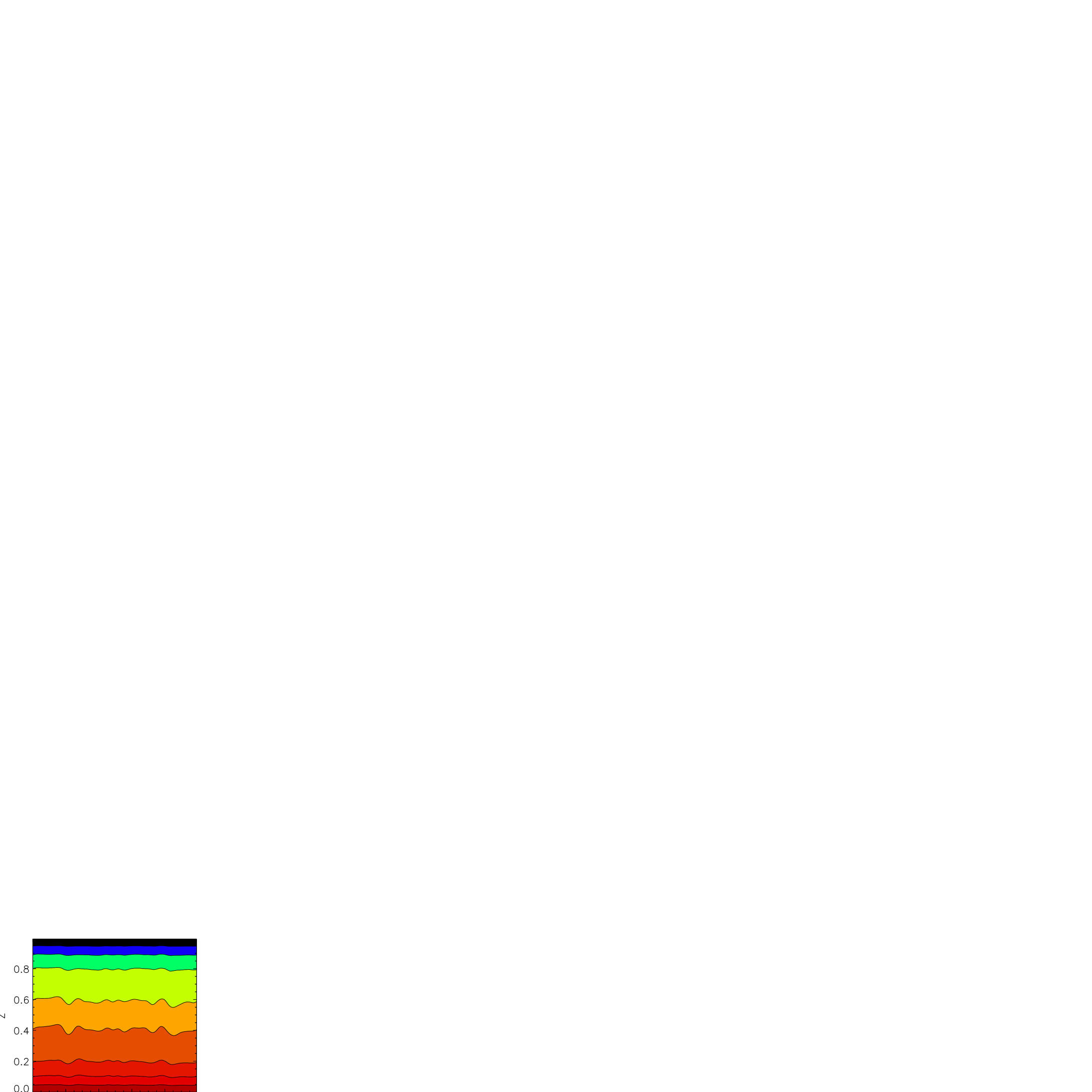
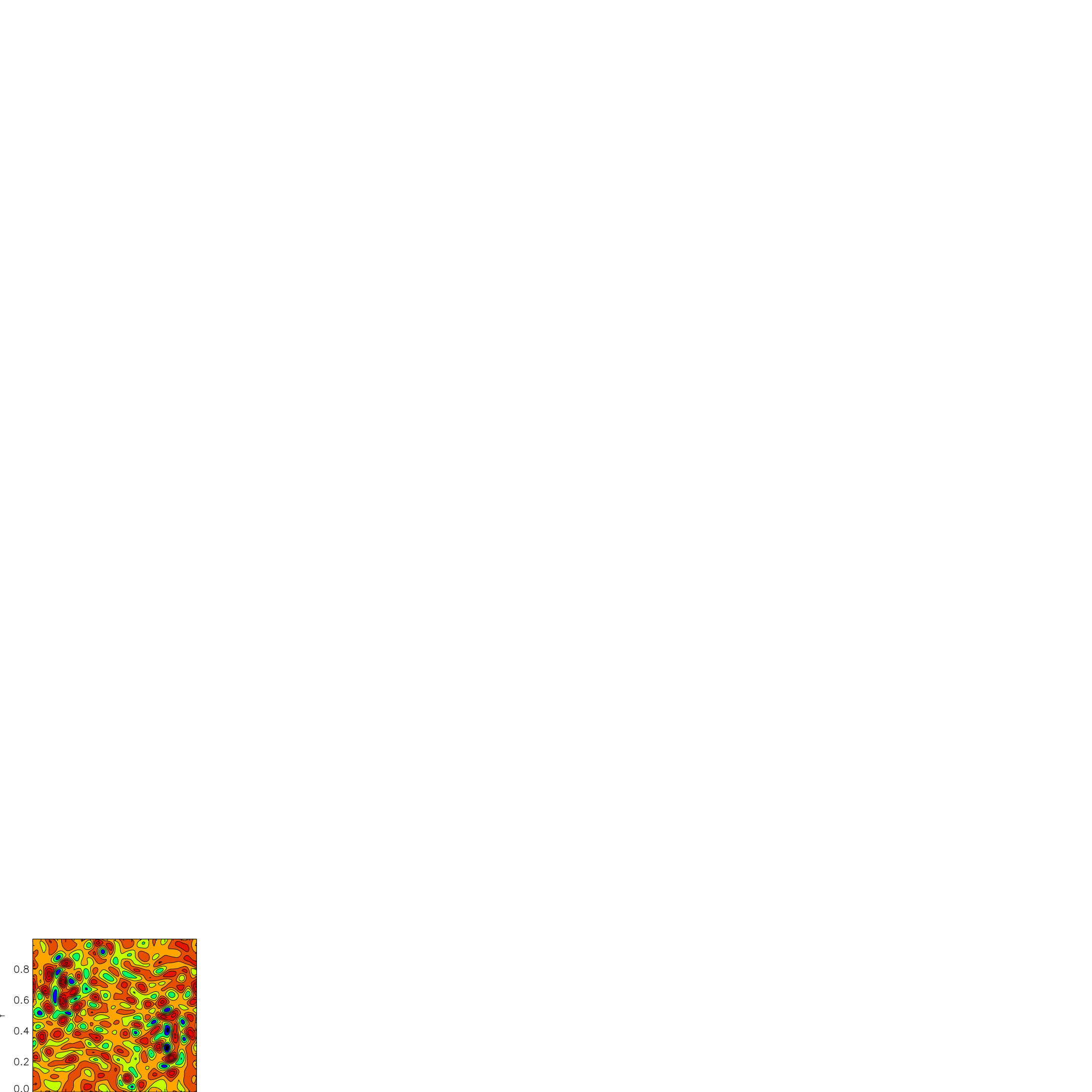
Abbildung 1: Regime R1. Sections of temperature distribution. . All sections correspond to the middle of the cube. The field ranges are $(0,\,1)$ – left, $(0.46,\,0.54)$ – right.

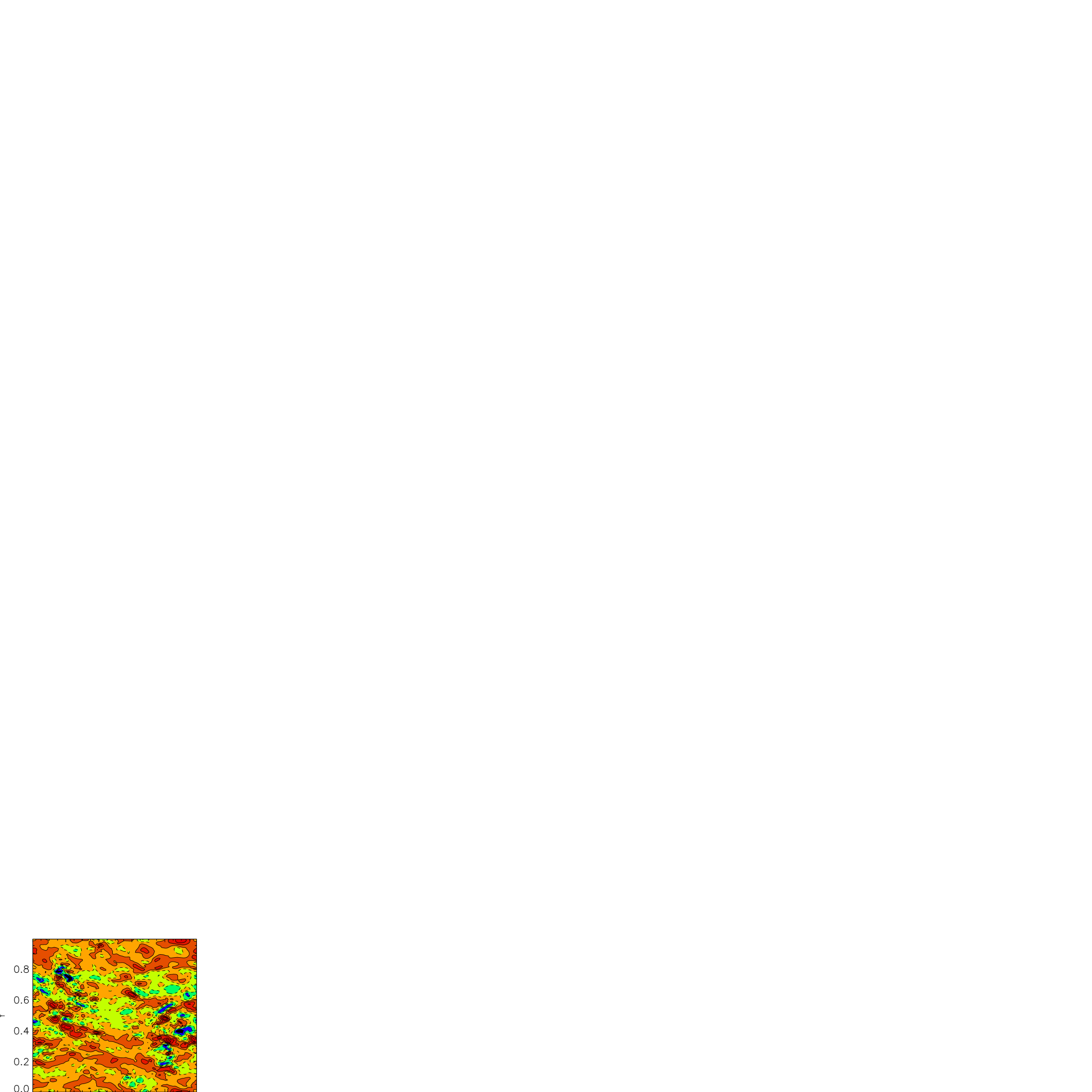
Abbildung 2: Distribution of $V_{x}$-component of the velocity field with ranges $(-248,\,253)$, $(-143,\,144)$.

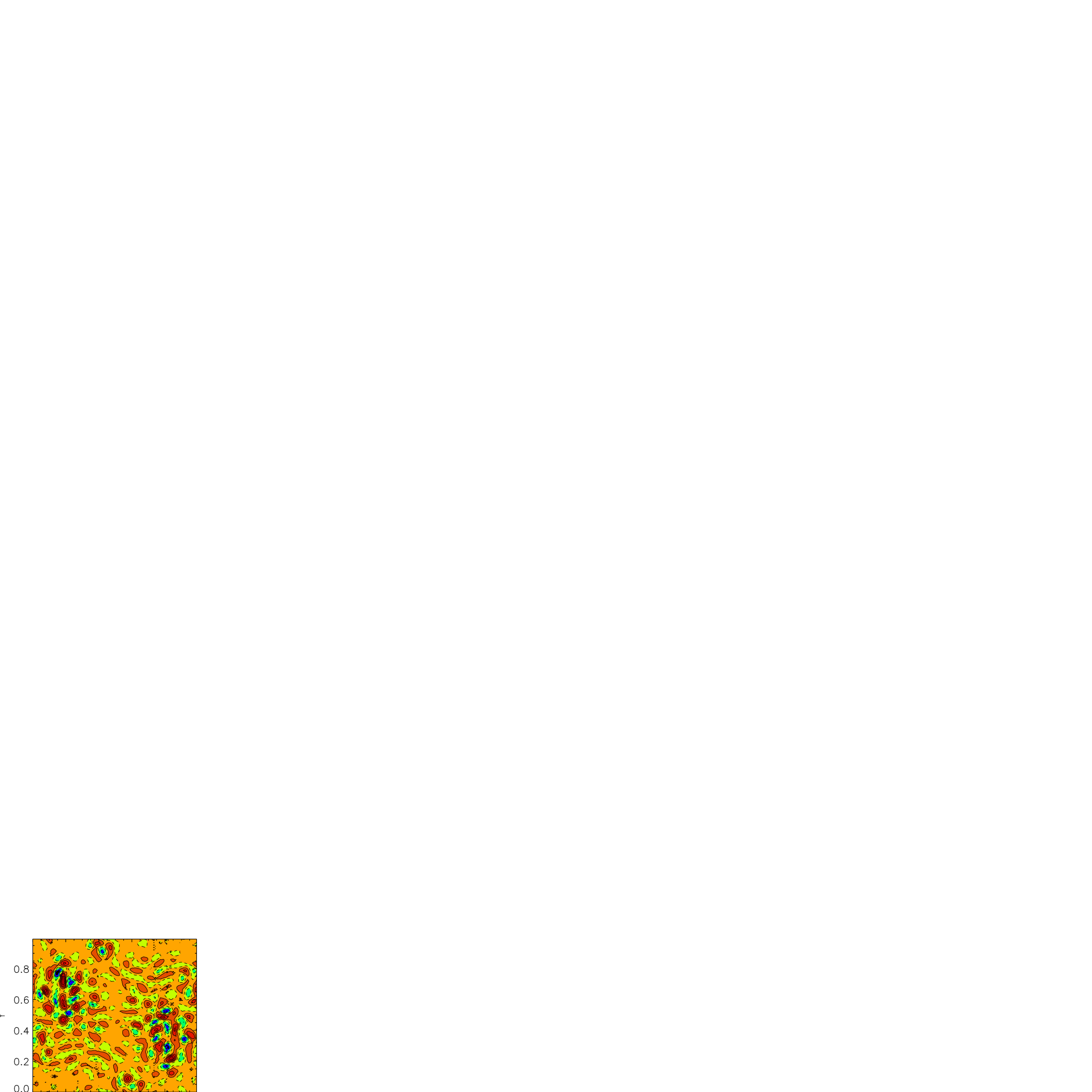
Abbildung 3: Distribution of $V_{z}$-component of the velocity field with ranges $(-675,\,701)$, $(-153,\,157)$

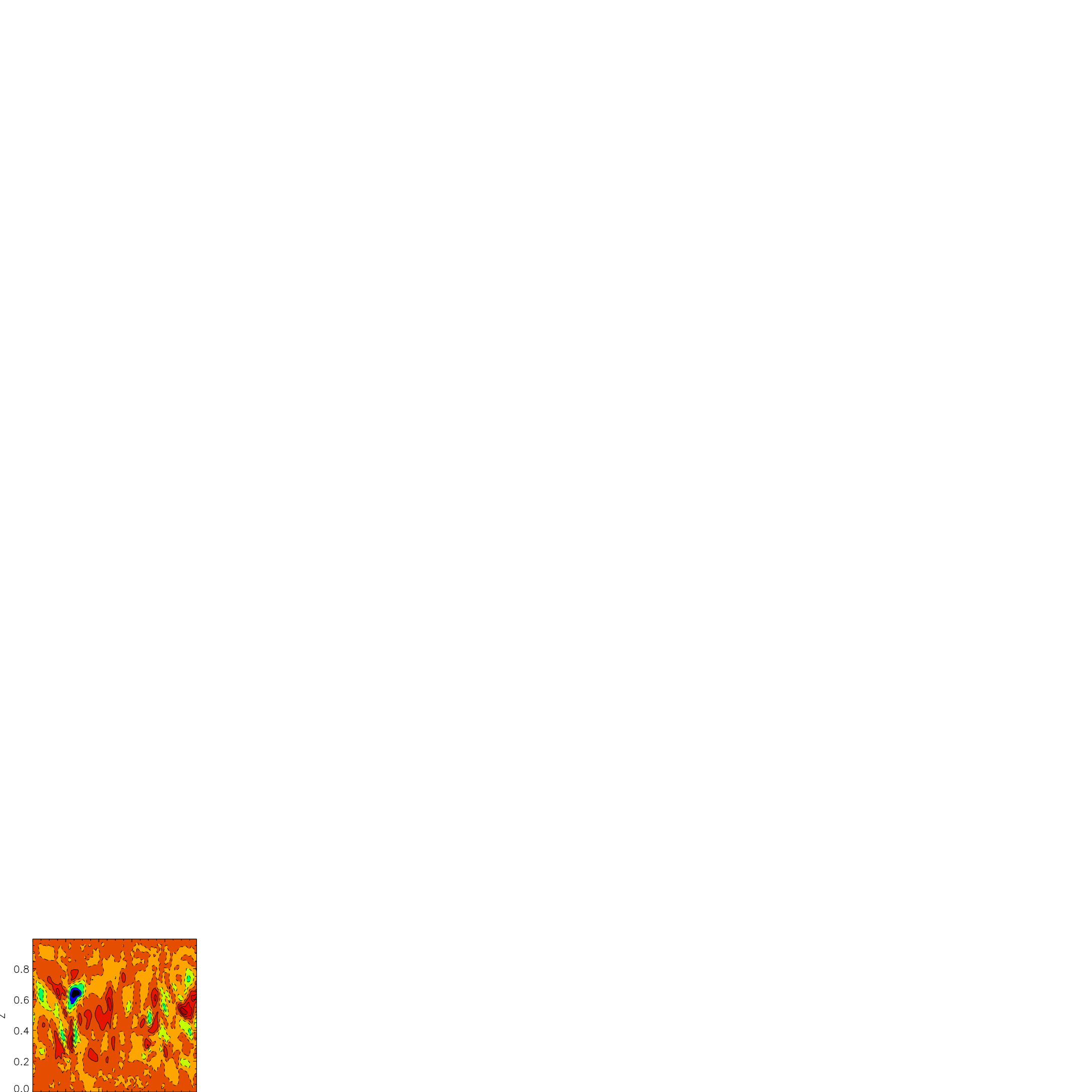
Abbildung 4: Distribution of $B_{z}$-component of the velocity field with ranges $(-1.44,\,1.14)$, $(-1.88,\,2.37)$

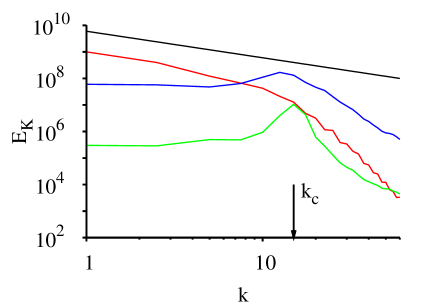
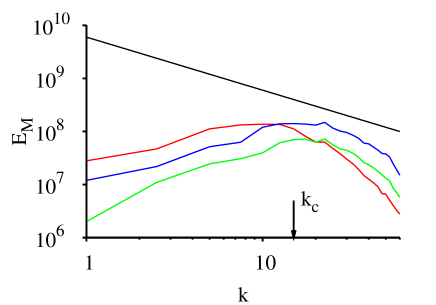
Abbildung 5: On the left is spectra of the kinetic energy for NR (red), R1 (green), R2 (blue). On the right is a spectra of the magnetic energy. The straight line corresponds to the Kolmogorov’s spectrum $\sim k^{-5/3}$.

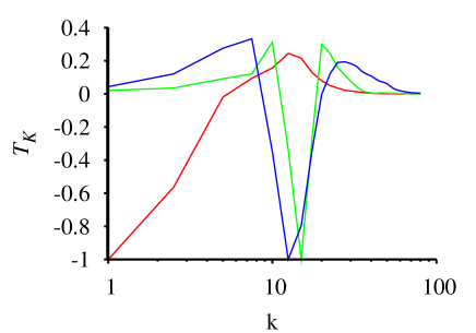
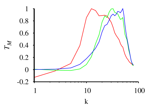
Abbildung 6: The normalized fluxes of kinetic ${T}_{K}$ (on the left) and magnetic ${T}_{M}$ (on the right) energies in the wave space: NR (red), R1 (green), R2 (blue).

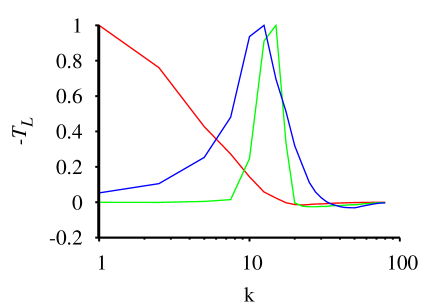
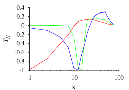
Abbildung 7: The normalized fluxes of the generation term $-{T}_{L}$ (on the left) and advective c ${T}_{N}$ (on the right) terms in the wave space: NR (red), R1 (green), R2 (blue).

2 Basic properties of the fields

Here we consider simulations without rotation similar to Meneguzzi and Pouquet (1989) and with rotation for two regimes with different amplitudes of the heat sources:

1. Regime without rotation, $\mathop{\rm Ra}\nolimits=6\cdot 10^{6}$, $\mathop{\rm Pr}\nolimits=1$, $\mathop{\rm E}\nolimits=1$, $\mathop{\rm q}\nolimits=10$, $\mathop{\rm Re}\nolimits\sim 2.5\cdot 10^{3}$.

2. Regime with rotation, $\mathop{\rm Ra}\nolimits=1.3\cdot 10^{3}$, $\mathop{\rm Pr}\nolimits=1$, $\mathop{\rm E}\nolimits=2\cdot 10^{-6}$, $\mathop{\rm q}\nolimits=10$, $\mathop{\rm Re}\nolimits\sim 1.6\cdot 10^{3}$.

3. Regime with rotation, $\mathop{\rm Ra}\nolimits=2.1\cdot 10^{3}$, $\mathop{\rm Pr}\nolimits=1$, $\mathop{\rm E}\nolimits=2\cdot 10^{-6}$, $\mathop{\rm q}\nolimits=10$, $\mathop{\rm Re}\nolimits\sim 3\cdot 10^{3}$.

The first (NR) regime is close to the typical Kolmogorov convection, see in more details Meneguzzi and Pouquet (1989). Including of rotation (regime R1) Fig. 1-5 leads to transform of the isotropic convective structures to the cyclonic state with horizontal scale $\sim\mathop{\rm E}\nolimits^{1/3}$ ($k_{c}\sim\mathop{\rm E}\nolimits^{-1/3}$) Chandrasekhar (1961). Including of the magnetic field (the full dynamo regime with magnetic energy comparable with the kinetic energy on the order of magnitude) does not change structure of the convective patterns too much Jones (2000). In the same time spectra of the magnetic energy are quite different and have no well-pronounced maximum at $k_{c}$.

Increase of Rayleigh number leads to decrease of the relative role of rotation and should decrease peak at the kinetic spectra energy what is accordance with spectra for regime R2, Fig. 5. In principle further increase of $\mathop{\rm Ra}\nolimits$ should lead to the original Kolmogorov state, similar to NR with spectrum law $\sim k^{-5/3}$ Fig. 5. However we emphasize, that information on the spectra is not enough to judge if the role of rotation is negligible or not and additional analysis is needed. The argument is the follows: rotation leads to degeneration of the third dimension (along z-axis) Batchelor (1953). On the other hand in isotropic two-dimensional systems spectraum of the kinetic energy also have $-5/3$-slope, however direction of the energy transfer in the system is inverse. In contrast to the three dimensional turbulence where energy transfers from the small wave number, where energy is injected, to larger dissipative wave number, in two dimensional turbulence energy transfers from the large wave numbers to the small ones. So far the quasi-geostrophic turbulence inherits properties of the both systems 2D and 3D, the inverse cascade Hossain (1994); Constantin (2002), we plan to consider behavior of energy fluxes in the wave space more carefully.

3 Energy fluxes

To analyze energy transfer in the wave space we follow Frisch (1995). Decompose physical field $f$ in sum of low-frequency and high-frequency counterparts: $f({\bf r})=f^{<}({\bf r})+f^{>}({\bf r})$, where

$$\begin{array}[]{l}\displaystyle f^{<}({\bf r})=\sum\limits_{|k|\leq K}\widehat{f}_{k}\,e^{i{\bf k}{\bf r}},\qquad f^{>}({\bf r})=\sum\limits_{|k|>K}\widehat{f}_{k}\,e^{i{\bf k}{\bf r}}.\end{array}$$ (6)

For any periodical $f$ and $g$ one has relation Frisch (1995):

$$\begin{array}[]{c}\displaystyle<{\partial f\over\partial x}>=0,\qquad<{\partial g\over\partial x}>=0,\\ \\ \displaystyle<g{\partial f\over\partial x}>=-<f{\partial g\over\partial x}>,\qquad<f^{>}g^{<}>=0,\end{array}$$ (7)

where

$$\begin{array}[]{c}\displaystyle<f({\bf r})>={\cal V}^{-1}\int\limits_{\cal V}f({\bf r})\,d{\bf r}^{3}\end{array}$$ (8)

means averaging of $f$ over the volume ${\cal V}$. Multiplying the Navier-Stokes equation by ${\bf V}^{<}$ and induction equation by ${\bf B}^{<}$ lead to equations of the integral fluxes of kinetic $E_{K}=V^{2}/2$ and magnetic $E_{M}=B^{2}/2$ energies from $k\geq K$ to $k<K$:

$$\begin{array}[]{c}\displaystyle\Pi_{K}=<\left({\bf V}\times{\rm rot}{\bf V}\right)\cdot{\bf V}^{<}>,\\ \\ \displaystyle\Pi_{M}=<{\rm rot}\left({\bf V}\times{\bf B}\right)\cdot{\bf B}^{<}>\end{array}$$ (9)

and for the flux of the Lorentz work:

$$\begin{array}[]{l}\displaystyle\Pi_{L}=<\left({\rm rot}{\bf B}\times{\bf B}\right)\cdot{\bf V}^{<}>.\end{array}$$ (10)

Introducing

$$\begin{array}[]{l}\displaystyle{T}_{K}(k)=-{\partial\Pi_{K}\over\partial k},\end{array}$$ (11)

leads to obvious relation for $E_{K}$ in $k$-space:

$$\begin{array}[]{l}\displaystyle{\partial E_{K}(k)\over\partial t}={T}(k)+F(k)+D(k),\end{array}$$ (12)

where $k=|{\bf k}|$, ${T}(k)$ is a flux of the energy from harmonics with different $k$, $F(k)$ is a work of the external forces and $D(k)=-k^{2}E_{K}(k)$ is a dissipation. The accurate form of ${T}$ is:

$$\begin{array}[]{l}\displaystyle{T}_{K}=-{\partial\Pi_{K}\over\partial k},\qquad\displaystyle\int\limits_{k=0}^{\infty}{T}_{K}(k)\,dk=0,\\ \displaystyle{T}_{M}={\partial\Pi_{M}\over\partial k},\qquad{T}_{L}={\partial\Pi_{L}\over\partial k}.\end{array}$$ (13)

Taking into account that ${\rm rot}\left({\bf V}\times{\bf B}\right)=-\left({\bf V}\cdot\nabla\right){\bf B}+\left({\bf B}\cdot\nabla\right){\bf V}$ one has: ${T}_{M}={T}_{N}-{T}_{L}$, where

$$\begin{array}[]{l}\displaystyle\par{T}_{N}=-{\partial\Pi_{N}\over\partial k},\qquad\displaystyle\int\limits_{k=0}^{\infty}{T}_{N}(k)\,dk=0,\\ \Pi_{N}=<\left(\left({\bf V}\cdot\nabla\right){\bf B}^{<}\right)\cdot{\bf B}^{<}>.\end{array}$$ (14)

Fig. 6 presents fluxes of kinetic ${T}_{K}$ and magnetic ${T}_{M}$ energies for the mentioned above regimes. Regime NR for ${T}_{K}$ demonstrates well-known behaviour for the direct Kolmogorov’s cascade in 3D. For the large scales ${T}_{K}<0$, these scales are donors, they provide energy to the system. On the other hand harmonics at the large $k$ absorb energy. The two-dimensional turbulence exhibits mirror-symmetrical behaviour relative to the axis of absciss Kraichnan and Montgomery (1980). In this case the energy cascade is inverse.

Rotation changes behaviour of fluxes of kinetic energy essentially. The leading order wave number is $k_{c}$. For $k>k_{c}$ we also observe the direct cascade of energy ${T}_{K}>0$. The maximum of ${T}_{K}$ is shifted relative to the maximum of the energy to the large $k$ as larger as larger $\mathop{\rm Re}\nolimits$. For $k<k_{c}$ behaviour is more complex: for the small $k$ the inverse cascade of the kinetic energy takes place ${T}_{K}>0$. On the other hand for the larger region of $k$ $(0\dots k_{c})$ we still have the direct cascade ${T}_{K}<0$. Increase of $\mathop{\rm Re}\nolimits$ leads to narrowing of the region with inverse cascade and increase of inverse flux. One can suggest, that change of the sign of the flux ${T}_{K}$ at $k<k_{c}$ is connected with appearance of the non-local energy transfer: so that energy to the large-scales ${\bf k_{1}}$ comes from modes $|{\bf k_{2}}|\sim|{\bf k_{3}}|\gg|{\bf k_{1}}|$, ${\bf k_{1}}={\bf k_{2}}+{\bf k_{3}}$ Waleffe (1992). In absence of the magnetic field maximum of ${T}_{K}(k=1)$ appears. So, in case with rotation there are two cascades of kinetic energy (direct and inverse) tale place simultaneously.

Now we consider the magnetic part. In contrast to ${T}_{K}$, ${T}_{M}$ includes not only advective term but the generative term as well. This leads to positiveness of the integral ${T}_{M}$ over all $k$. Moreover ${T}_{M}$ is positive for any $k$. Position of maximum of ${T}_{M}$ is close to that ones in spectra of $E_{M},\,{T}_{K}$.

It is evident, that for the planetary cores distance between maxima in fluxes ${T}_{M}$ for NR and R1, R2 can be quite large, however not so large as $k_{c}$. This statement concerned with condition on magnetic field generation which holds when the local magnetic Reynolds number ${\rm r_{m}}>1$ at the scale $1/k$: $\displaystyle{\rm r_{m}}={v_{k}\over k\eta}>1$ and that for the planets $\eta\gg\nu$. In the same moment fluxes at the small $k$ are small, i.e. system is in the state of the statistical equilibrium: dissipation at the small scales is negligible.

Now we examine the origin of the magnetic energy at the scale $1/k$: does it concerned with the energy transfer from the other scales either it is a product of real generation at this scale?

Fig. 7 demonstrates fluxes of $-{T}_{L}$, concerned with magnetic field generation. The maximum of generation term without rotation is at the large scale, while for the rotating system it is at $\sim 1/k_{c}$. Interestingly, that for the rotating system there is a region $-{T}_{L}<0$ for the large $k$, where magnetic field reinforce convection. For regime NR $-{T}_{L}$ drops quickly because of the kinetic energy decrease Fig. 5. As a result we have: for the rotating system magnetic field is produced by the cyclones, while for the non-rotating system the large-scale dynamo operates.

Now we estimate the role of the advective term ${T}_{N}$ separately. For the non-rotating ${T}_{N}$ and ${T}_{K}$ are similar: the direct cascade takes place. For rotating system region $k\sim k_{c}$ is a source of energy. In contrast to ${T}_{K}$, ${T}_{N}$ has not positive regions at the small $k$, i.e. the inverse cascade of the magnetic energy, concerned with the advective term in this region is absent. We draw attention to the amplitudes of the fluxes ${T}_{M}$, $-{T}_{L}$, ${T}_{N}$: for all three cases hold $\displaystyle{{|T}_{M}|\over|{T}_{L}|}\sim 10^{-1}$, i.e. two fluxes of the magnetic energy in the wave space with opposite directions exist. The first flux concerned with the traditional energy transfer of the energy over the spectrum (advective term) and the flux of the Lorentz work. The regions of the maximal magnetic field generation coincide with the regions of the most effective magnetic energy transfer ${T}_{N}$ (from small $k$ to the large $k$). Such a balance leads to equipartition state, when dissipation takes place on the large $k$.

Note, that the full magnetic flux Fig. 6 ${T}_{M}$ is localized at $k\gg 1$. For the non-rotating system it is because the mean helicity and $\alpha$-effect are zero Zeldovich et al. (1983). Thus the inverse cascade of the magnetic energy to the small $k$ is absent.

For the rotating system here is a balance of the energy injection due to the Lorentz force and its wash-out because of advection. The latest effect reduces $\alpha$-effect.

The magnetic fields of the planets are the main sources of information on the processes in the liquid cores at the times $10^{2}-10^{3}$yy and more. If the poloidal part of the magnetic field is observable at the planet surface, then the largest component of field (toroidal) as well as the kinetic energy distrubution over the scales is absolutely invisible for the observer out of the core. Moreover, due to finite conductivity of the mantle even the poloidal part of the magnetic field is cutted off at $k\ll k_{c}$. In other words the observable part of the spectra at the planets surface is only a small part (not even the largest) of the whole spectra of the field. That is why importance of the numerical simulation is difficult to overestimate. Here we showed that in considered quasigeostrophic state the both cascades (direct and inverse) exsist simulataneously. That is a challenge for a turbulent models in the geodynamo. The other interesting point is a balance of the magnetic energy flux due two mechanisms: advection and generation. This balance is reason why the exponential growth of the magnetic energy is stopped at the end of the kinematic dynamo regime.