Finite temperature quantum statistics of H${}_{3}^{+}$ molecular ion

Abstract

Full quantum statistical $NVT$ simulation of the five-particle system H${}_{3}^{+}$ has been carried out using the path integral Monte Carlo method. Structure and energetics is evaluated as a function of temperature up to the thermal dissociation limit. The weakly density dependent dissociation temperature is found to be around $4000$ K. Contributions from the quantum dynamics and thermal motion are sorted out by comparing differences between simulations with quantum and classical nuclei. The essential role of the quantum description of the protons is established.

I Introduction

The triatomic molecular ion H${}_{3}^{+}$ is a five-body system consisting of three protons and two electrons. Being the simplest polyatomic molecule it has been the subject of a number of theoretical and experimental studies over the years Oka (1992); Gottfried et al. (2003); Kutzelnigg and Jaquet (2006); Kreckel et al. (2008); Pavanello and Adamowicz (2009). Experimentally, the H${}_{3}^{+}$ ion was first detected in 1911 by Thompson Thomson (1911), however, definite spectroscopic studies were carried out not until 1980 by Oka Oka (1980). Since then, this five-body system has proven to be relevant, also in astrophysical studies concerning the interstellar media and the atmosphere of gas planets. Therefore, low-density high-temperature H${}_{3}^{+}$ ion containing atmospheres have been studied experimentally Lystrup et al. (2008) as well as computationally Koskinen et al. (2009).

Until now, the computational approaches have consistently aimed at finding ever more accurate potential energy surfaces (PES) for H${}_{3}^{+}$ at zero Kelvin, and consequent calculations of the rovibrational states Meyer et al. (1986); Röhse et al. (1994). These calculations include Born–Oppenheimer (BO) electronic energies in various geometries often supplemented with adiabatic and relativistic corrections Cencek et al. (1998); Bachorz et al. (2009). For the study of rovibrational transitions it is desirable to have an analytical expression for the PES, which is usually generated using Morse polynomial fits Meyer et al. (1986). Inclusion of the nonadiabatic effects, however, has turned out to be a cumbersome task, and so far, they have not been rigorously taken into account Pavanello and Adamowicz (2009).

In this work, we evaluate the full five-body quantum statistics of the H${}_{3}^{+}$ ion in a stationary state at temperatures below the thermal dissociation at about $4000$ K. We use the path integral Monte Carlo (PIMC) approach, which allows us to include the Coulomb correlations between the particles exactly in a transparent way. Thus, we are able to monitor the fully nonadiabatic correlated quantum distributions of particles and related energies as a function of temperature. Furthermore, we are able to model the nuclei as classical mass points, in thermal motion or fixed as conventionally in quantum chemistry, and find the difference between these and the quantum delocalized nuclei.

The PIMC method is computationally expensive, but within the chosen models and numerical approximations it has been proven to be useful with exact correlations and finite temperature Li and Broughton (1987); Ceperley (1995); Pierce and Manousakis (1999); Kwon and Whaley (1999); Knoll and Marx (2000); Cuervo and Roy (2006); Kylänpää et al. (2007); Kylänpää and Rantala (2009). For zero Kelvin data with benchmark accuracies, however, the conventional quantum chemistry or other Monte Carlo methods, such as the diffusion Monte Carlo Anderson (1992), are more appropriate. Thus, it should be emphasized that we do not aim at competing in precision or number of decimals with the other approaches. Instead, we will concentrate on physical phenomena behind the finite-temperature quantum statistics.

Next, we will briefly describe the basics of the PIMC method and the model we use for the ion. In the results and discussion section we first compare our $160$ K PIMC "ground state" to the zero Kelvin ground state, and then, consider the higher temperature effects.

II Method

According to the Feynman formulation of the quantum statistical mechanics Feynman (1998) the partition function for interacting distinguishable particles is given by the trace of the density matrix:

$$Z=\text{Tr}\leavevmode\nobreak\ \hat{\rho}(\beta)=\int\text{d}R_{0}\text{d}R_{1}\ldots\text{d}R_{M-1}\prod_{i=0}^{M-1}e^{-S(R_{i},R_{i+1};\tau)},$$

where $\hat{\rho}(\beta)=e^{-\beta\hat{H}}$, $S$ is the action, $\beta=1/k_{\text{B}}T$, $\tau=\beta/M$, $R_{M}=R_{0}$ and $M$ is called the Trotter number. In this paper, we use the pair approximation in the action Storer (1968); Ceperley (1995) for the Coulomb interaction of charges. Sampling in the configuration space is carried out using the Metropolis procedure Metropolis et al. (1953) with bisection moves Chakravarty et al. (1998). The total energy is calculated using the virial estimator Herman et al. (1982).

The error estimate in the PIMC scheme is commonly given in powers of the imaginary time time-step $\tau$.Ceperley (1995) Therefore, in order to systematically determine thermal effects on the system we have carried out all the simulations with $\tau=0.03E_{\text{H}}^{-1}$, where $E_{\text{H}}$ denotes the unit of Hartree. Thus, the temperatures and Trotter number $M$ become fixed by the relation $T=(k_{\text{B}}M\tau)^{-1}$.

In the following we mainly use the atomic units, where the lengths, energies and masses are given in units of the Bohr radius ($a_{0}$), Hartree ($E_{\text{H}}$) and free electron mass ($m_{e}$), respectively.

The statistical standard error of the mean (SEM) with $2$SEM limits is used as an error estimate for the observables, unless otherwise mentioned.

III Models

Two of the five particles composing the H${}_{3}^{+}$ ion are electrons. For these, we do not need to sample the exact Fermion statistics, but it is sufficient to assign spin-up to one electron and spin-down to the other one. This is accurate enough, as long as the thermal energy is well below that of the lowest electronic triplet excitation.

We do the same approximation for the three protons, too. This is even more safe, because the overlap of well localized nuclear wave functions is negligible and related effects become very hard to evaluate, anyway. On the other hand, however, the nuclear exchange due to the molecular rotation results in the so called zero-point rotations. These too contribute to energetics less than the statistical accuracy of our simulations. Therefore, we ignore the difference between ortho-H${}_{3}^{+}$ ($I=3/2$) and para-H${}_{3}^{+}$ ($I=1/2$). Thus, the protons are modeled as "boltzmannons" with the mass $m_{p}=1.83615267248\times 10^{3}m_{e}$. The higher the temperature, the better is the Boltzmann statistics in describing the ensemble composed of ortho- and para-H${}_{3}^{+}$.

For the $NVT$ simulations we place one H${}_{3}^{+}$ ion into a cubic box with the volume of $(300a_{0})^{3}$ and apply periodic boundary conditions (PBC) and minimum image principle. This corresponds to the mass density of $\sim 1.255\times 10^{-6}\leavevmode\nobreak\ \rm{gcm}^{-3}$. This has no essential effect at low $T$, but at high $T$ the finite density gives rise to the molecular recombination balancing the possible dissociation. Within the considered temperature range the dissociations are very rare.

The electrons are always simulated with the full quantum dynamics. For the nuclei, however, we use three models to trace the quantum and thermal fluctuations, separately. The case of full quantum dynamics of all particles we denote by AQ (all-quantum), the mass point model of protons by CN (classical nuclei) and the adiabatic case of fixed nuclei by BO (Born–Oppenheimer potential energy surface).

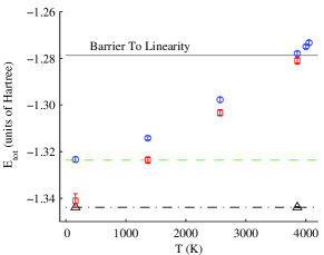
Figure 1: (Color online) Total energy of the H${}_{3}^{+}$ molecular ion as a function of temperature. Fully nonadiabatic quantum statistical simulations, AQ (blue circles), classical nuclei simulations, CN (red squares), and the equilibrium geometry Born–Oppenheimer simulation, BO (black triangles). Zero Kelvin data Kutzelnigg and Jaquet (2006); Pavanello and Adamowicz (2009); Röhse et al. (1994) is given for comparison: BO ground state energy at equilibrium internuclear geometry (black dash-dotted line), energy including the nuclear zero-point motion (green dashed line) and energy at the barrier to linearity (grey solid line). $2$SEM statistical error estimate is shown by the error bars from simulations at the H${}_{3}^{+}$ ion density $(300a_{0})^{3}$ or $\sim 1.255\times 10^{-6}\leavevmode\nobreak\ \rm{gcm}^{-3}$.

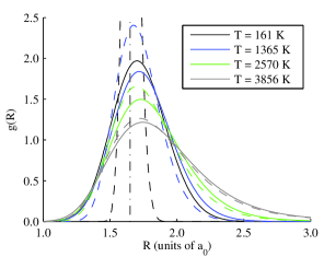
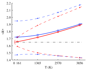
Figure 2: (Color online) Nuclear pair correlation functions (bond length distributions) at different temperatures from the quantum statistical simulations (solid lines), and from the classical nuclei simulations (dashed lines). The zero Kelvin equilibrium internuclear distance is given as a vertical black dash-dotted line. The distributions include the $r^{2}$ weight and normalization to unity. (Note that the $r^{2}$ weight is usually not included in description of extended or periodic systems)

Figure 3: (Color online) Expectation values of the internuclear distance at different temperatures from distributions in Fig. 3. Quantum statistical simulations (blue circles) and classical nuclei simulations (red squares). The FWHM limits are shown by triangles (all the lines are for guiding the eye). The zero Kelvin equilibrium internuclear distance is shown as a horizontal black dash-dotted line.

IV Results and discussion

IV.1 Ground state: zero Kelvin reference data

The equilibrium geometry of the H${}_{3}^{+}$ ion in its ground state is an equilateral triangle $D_{3h}$ for which the internuclear equilibrium distance is $R=1.65a_{0}$ Pavanello and Adamowicz (2009). The best upper bound for the electronic ground state BO energy to date is $-1.34383562502E_{\text{H}}$ Pavanello and Adamowicz (2009). The vibrational normal modes of H${}_{3}^{+}$ are the symmetric-stretch mode $\nu_{1}$ and the doubly degenerate bending mode $\nu_{2}$. The latter one breaks the full symmetry of the molecule, and therefore, it is infrared active Kreckel et al. (2008).

The vibrational zero-point energy is $0.01987E_{\text{H}}$, and the so called rotational zero-point energies are $0.00029E_{\text{H}}$ and $0.00040E_{\text{H}}$ for para- and ortho-H${}_{3}^{+}$, respectively Röhse et al. (1994); Kutzelnigg and Jaquet (2006). These yield about $0.020215E_{\text{H}}$ for the average zero-point energy. Note however, that the nuclear spins and zero point rotation are not included in our model of H${}_{3}^{+}$.

The lowest electronic excitation from the BO ground state is a direct Franck–Condon one ($0.710E_{\text{H}}$)Pavanello and Adamowicz (2009); Kreckel et al. (2008) to dissociative potential curve: $\text{H}_{3}^{+}\rightarrow\text{H}_{2}+\text{H}^{+}$ or $\text{H}_{3}^{+}\rightarrow\text{H}_{2}^{+}+\text{H}$. Viegas et al. (2007); Pavanello and Adamowicz (2009) The dissociation energies ($D_{e}$) are $0.169E_{\text{H}}$ and $0.241E_{\text{H}}$, respectively.

The linear geometry with equal bond lengths $1.53912a_{0}$ ($D_{\infty h}$) is a saddle point on the BO PES at $-1.27868190E_{\text{H}}$ Röhse et al. (1994) or $0.06515E_{\text{H}}$ above the BO energy at the equilibrium geometry. This energy is usually called as the barrier to linearity Gottfried et al. (2003). The zero Kelvin energetics is shown in Fig. 1 by the three horizontal lines.

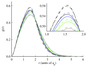
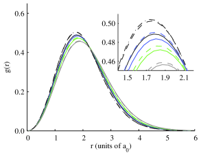
Figure 4: (Color online) Proton–electron pair correlation functions at the four temperatures from the full quantum statistical simulations, AQ (solid lines), and from simulations with the classical nuclei, CN (dashed lines). That from the BO scheme is given at the lowest (electronic) temperature, only (dash-dotted line). Notations are the same as in Fig. 3.

Figure 5: (Color online) Electron–electron pair correlation functions from the same simulations as those in Fig. 5. Notations are the same as in Figs. 3 and 5.

IV.2 PIMC ground state: 160 K

At our lowest simulation temperature, $T\approx 160$ K, the electronic system is essentially in its ground state. For the total energy we find $-1.3438(2)E_{\text{H}}$, see the BO black triangles in Fig. 1. The thermal energy is $k_{B}T=0.000507E_{\text{H}}$, and therefore, the contribution from the rotational and vibrational excited states is also small and we find $-1.3406(29)E_{\text{H}}$, see the CN red square in same Fig. The full quantum simulation includes vibrational zero-point contribution and yields $-1.3233(12)E_{\text{H}}$, about $0.0205(14)E_{\text{H}}$ above the BO energy in a good agreement with about $0.0202E_{\text{H}}$ in Refs. Röhse et al. (1994); Kutzelnigg and Jaquet (2006).

From our AQ simulation we still find the equilateral triangle configuration of the nuclei with the internuclear distances increased to $\langle R\rangle=1.723(4)a_{0}$, which indicates an increase of about $0.073(4)a_{0}$, as compared with the zero Kelvin BO equilibrium distance bond lengths. Interestingly, within the error limits this is the same as the bond length increase of the hydrogen molecule ion H${}_{2}^{+}$. The zero-point energy of H${}_{3}^{+}$ is about $2.7$ times as large as that of the H${}_{2}^{+}$ ion Kylänpää et al. (2007), as expected from the increase of vibrational modes from one to three — the zero-point energy of our model does not contain the rotational zero-point energy, as mentioned earlier.

The thermal motion (CN), alone, increases the bond length to $\langle R\rangle=1.658(4)a_{0}$, only, see the data in Figs. 3 and Fig. 3. This clearly points out the difference between quantum and thermal delocalization of nuclei at low $T$.

For the proton–electron and electron–electron interactions the differences between our two approaches are smaller than in the proton–proton case but still distinctive. Comparison of the fixed nuclei simulation to the CN one shows that the two schemes give almost identical distributions. The AQ distributions, however, cannot be labeled identical with those from the CN or fixed nuclei simulations. The distributions are given in Figs. 5 and 5, where the notations are the same as in Fig. 3.

The calculations of the relativistic corrections involve, among other things, evaluation of the contact densities, $\langle\delta(r_{ij})\rangle$, for the electron–nuclei and the electron–electron pairs Cencek et al. (1998). For the electron–nuclei contact density at the BO equilibrium configuration we get $0.1814(20)$, and for the AQ case $0.1765(20)$. For the electron–electron pair we get $0.0182(3)$ and $0.0166(3)$, for BO and AQ approaches respectively. The estimated uncertainties due to extrapolation to the contact are given in parenthesis. The zero Kelvin reference values Cencek et al. (1998) for the BO case are $0.181242$ (electron–nuclei) and $0.01838663$ (electron–electron). Thus, the quantum dynamics of the nuclei turns out to be significant factor in lowering the contact densities, too.

See the snapshot of the AQ simulation in Fig. 6 for some intuition of the low-temperature quantum distributions in imaginary time.

Table 1: Energetics of the H${}_{3}^{+}$ molecular ion. The energies are given in the units of Hartree (atomic units). Simulation data is given with $2$SEM error estimates. BO refers to Born–Oppenheimer calculation at equilibrium geometry. The reference data is rounded to convenient accuracy. The "barrier to linearity" is $0.06515E_{\text{H}}\approx 1.8$ eV above the $E_{\text{BO}}$ at $0$ K.

	$T$	$E_{\text{BO}}$	$E_{\text{CN}}$	$E_{\text{AQ}}$
Ref. Pavanello and Adamowicz (2009)	$0$ K	$-1.343836$		$-1.323568$
PIMC	$\sim 161$ K	$-1.3438(2)$	$-1.3406(29)$	$-1.3233(12)$
PIMC	$\sim 1365$ K		$-1.3236(8)$	$-1.3142(4)$
PIMC	$\sim 2570$ K		$-1.3033(7)$	$-1.2977(6)$
PIMC	$\sim 3856$ K	$-1.3438(2)$	$-1.2810(8)$	$-1.2770(2)$
PIMC	$\sim 3999$ K		$-1.1469(9)$	$-1.2750(4)$
PIMC	$\sim 4050$ K			$-1.2734(9)$

IV.3 High temperature phenomena

With the increasing temperature the increasing contribution from rovibrational excitations is clearly seen in the total energies shown in Fig. 1. Contributions from the electronic excitations do not appear, because the lowest excitation energy $0.710E_{\text{H}}$ is much too high as compared to the thermal energy $k_{B}T$. Consequently, the equilibrium geometry BO energy depends on the temperature almost negligibly. For convenience, the essential energetics related data has been collected into Table 1, also.

As expected, the increase in the total energy due to the classical rovibrational degrees of freedom is $9\times\tfrac{1}{2}k_{B}T$, defining the slope of the CN line. The most prominent quantum feature in AQ curve is, of course, the zero-point vibration energy. At higher temperatures, however, by comparing the AQ and CN curves we see that the quantum nature of nuclear dynamics becomes less important, except for dissociation.

At the dissociation limit we find the molecule with quantum nuclei somewhat more stable than the one with classical nuclei. With the relatively low density, $(300a_{0})^{3}$, the molecule is mainly kept in one piece above $4000$ K in the former case, whereas more dissociated in the latter. The total energy becomes higher for the CN than the AQ case slightly below $4000$ K, see Table 1. The total energies at this crossing point are above the "barrier to linearity",Röhse et al. (1994); Gottfried et al. (2003) already.

At higher temperatures, $T\geq 4100$ K, other configurations, such as $\text{H}_{2}+\text{H}^{+}$, $\text{H}_{2}^{+}+\text{H}$ and $2\text{H}+\text{H}^{+}$, start playing more significant role in the equilibrium dissociation–recombination processes. These will considered in our next study.

The nuclear pair correlation function or bond length distributions, Figs. 3 and 3, follow the energetics discussed, above. There, the zero-point vibration in AQ case is seen even better. At the zero Kelvin limit both the expectation value and the distribution, in particular, are significantly different from those of the CN case.

The temperature dependence in the other pair correlation functions is weak, see Figs. 5 and 5. Obviously, this is the case, because electrons do not present a quantum-to-classical transition in the temperature range considered, now. Thus, the evolution in distributions in Figs. 5 and 5 following the rising temperature arises from the changes in the nuclear dynamics, and mostly, from the change in the conformation or the bond lengths, presented in Fig. 3.

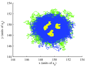
Figure 6: (Color online) xy-plane (z-projection) snapshot of the H${}_{3}^{+}$ ion from quantum statistical simulation with Trotter number $2^{16}$, i.e. temperature of about $160$ K, for all particles. ”Polymer rings” describing the electrons are in the background (green and blue) and those of the nuclei are placed on top (yellow).

V Conclusions

In this study, the path integral Monte Carlo method was shown to be a successful approach for examination of quantum statistics of the five-particle molecule, H${}_{3}^{+}$ ion. The method is based on the finite temperature mixed state description, and thus, it gives information, which is complementary to the high-accuracy zero Kelvin description of conventional quantum chemistry. It was also shown how contributions from quantum and thermal dynamics to particle distributions and correlation functions can be sorted out, and furthermore, quantum to classical dynamics transition can be monitored.

Our approach is fully basis set and trial wave function free. It is based on the Coulomb interactions, only, and allows the most transparent interpretation of consequent particle–particle correlations.

Simulation at $160$ K essentially reproduces the zero Kelvin data from conventional quantum chemistry. Of course, a proper extrapolation to $0$ K can be done for more accuracy. Born–Oppenheimer (BO) potential energy surface and the equilibrium geometry can be found by using classical nuclei with fixed coordinates. Description of the zero-point motion within our nonadiabatic five-body quantum simulation gives the vibrational zero-point energy accurately. We find an increase of $0.073(4)a_{0}$ in the bond length due to the nonadiabatic zero-point vibration. The classical thermal contribution at $160$ K is $0.008(4)a_{0}$, only.

With the raising temperature the rovibrational excitations contribute to the energetics, as expected, whereas the electronic part remains in its ground state in the spirit of BO approximation. At about $4000$ K the H${}_{3}^{+}$ ion dissociates, weakly depending on the ion density. We find that the full quantum molecule dissociates at slightly higher temperature compared to the one, where the nuclei are modeled by classical particles with thermal dynamics, only. Thus, we conclude the necessity of the quantum character of the protons in the correct description of dissociation.

We find that the nuclear quantum dynamics has a distinctive effect on the pair correlation functions, too. This is least for the electron–electron pair correlation function, stronger for the electron–proton one and largely increased in the proton–proton correlations. These are seen in the contact densities, and consequently, in the relativistic corrections where relevant.

VI Acknowlegements

For financial support we thank the Academy of Finland, and for computational resources the facilities of Finnish IT Center for Science (CSC) and Material Sciences National Grid Infrastructure (M-grid, akaatti). We also thank Kenneth Esler and Bryan Clark for their advise concerning the pair approximation.

References

- Oka (1992) T. Oka, Rev. Mod. Phys. 64, 1141 (1992).
- Gottfried et al. (2003) J. L. Gottfried, B. J. McCall, and T. Oka, J. Chem. Phys. 118, 10890 (2003).
- Kutzelnigg and Jaquet (2006) W. Kutzelnigg and R. Jaquet, Phil. Trans. R. Soc. A 364, 2855 (2006).
- Pavanello and Adamowicz (2009) M. Pavanello and L. Adamowicz, J. Chem. Phys. 130, 034104 (2009).
- Kreckel et al. (2008) H. Kreckel, D. Bing, S. Reinhardt, A. Petrignani, M. Berg, and A. Wolf, J. Chem. Phys. 129, 164312 (2008).
- Thomson (1911) J. J. Thomson, Philos. Mag. 21, 225 (1911).
- Oka (1980) T. Oka, Phys. Rev. Lett. 45, 531 (1980).
- Lystrup et al. (2008) M. B. Lystrup, S. Miller, N. D. Russo, J. R. J. Vervack, and T. Stallard, Astrophys. J. 677, 790 (2008).
- Koskinen et al. (2009) T. T. Koskinen, A. D. Aylward, and S. Miller, Astrophys. J. 693, 868 (2009).
- Meyer et al. (1986) W. Meyer, P. Botschwina, and P. Burton, J. Chem. Phys. 84, 891 (1986).
- Röhse et al. (1994) R. Röhse, W. Kutzelnigg, R. Jaquet, and W. Klopper, J. Chem. Phys. 101, 2231 (1994).
- Cencek et al. (1998) W. Cencek, J. Rychlewski, R. Jaquet, and W. Kutzelnigg, J. Chem. Phys. 108, 2831 (1998).
- Bachorz et al. (2009) R. A. Bachorz, W. Cencek, R. Jaquet, and J. Komasa, J. Chem. Phys. 131, 024105 (2009).
- Li and Broughton (1987) X.-P. Li and J. Q. Broughton, J. Chem. Phys 86, 5094 (1987).
- Ceperley (1995) D. M. Ceperley, Rev. Mod. Phys 67, 279 (1995).
- Pierce and Manousakis (1999) M. Pierce and E. Manousakis, Phys. Rev. B 59, 3802 (1999).
- Kwon and Whaley (1999) Y. Kwon and K. B. Whaley, Phys. Rev. Lett. 83, 4108(4) (1999).
- Knoll and Marx (2000) L. Knoll and D. Marx, Europ. Phys J. D 10, 353 (2000).
- Cuervo and Roy (2006) J. E. Cuervo and P.-N. Roy, J. Chem. Phys. 125, 124314 (2006).
- Kylänpää and Rantala (2009) I. Kylänpää and T. T. Rantala, Phys. Rev. A 80, 024504 (2009).
- Kylänpää et al. (2007) I. Kylänpää, M. Leino, and T. T. Rantala, Phys. Rev. A 76, 052508(7) (2007).
- Anderson (1992) J. Anderson, J. Chem. Phys. 93, 3702 (1992).
- Feynman (1998) R. P. Feynman, Statistical Mechanics (Perseus Books, 1998).
- Storer (1968) R. G. Storer, J. Math. Phys. 9, 964 (1968).
- Metropolis et al. (1953) N. Metropolis, A. W. Rosenbluth, M. N. Rosenbluth, A. H. Teller, and E. Teller, J. Chem. Phys. 21, 1087 (1953).
- Chakravarty et al. (1998) C. Chakravarty, M. C. Gordillo, and D. M. Ceperley, J. Chem. Phys. 109, 2123 (1998).
- Herman et al. (1982) M. F. Herman, E. J. Bruskin, and B. J. Berne, J. Chem. Phys. 76, 5150 (1982).
- Viegas et al. (2007) L. P. Viegas, A. Alijah, and A. J. C. Varandas, J. Chem. Phys. 126, 074309 (2007).