Radiative-nonrecoil corrections of order $\alpha^{2}(Z\alpha)E_{F}$ to the hyperfine splitting of muonium

Abstract

We present results for the corrections of order $\alpha^{2}(Z\alpha)E_{F}$ to the hyperfine splitting of muonium. We compute all the contributing Feynman diagrams in dimensional regularization and a general covariant gauge using a mixture of analytical and numerical methods. We improve the precision of previous results.

I Introduction

Muonium is the hydrogenlike bound state of a positive muon and an electron. Unlike hydrogen, or any other bound state involving hadrons, muonium is free from the complications introduced by the finite size or the internal structure of any of its constituents. Therefore, it allows for a very precise test of bound-state QED, and can be used to restrict models of physics beyond the Standard Model. Measurements of the ground-state hyperfine splitting of muonium are used to extract the muon to electron mass ratio $m_{\mu}/m_{e}$ and the muon to proton magnetic moment ratio $\mu_{\mu}/\mu_{p}$ Mohr:2008fa . The value of $\mu_{\mu}/\mu_{p}$ is required for obtaining the muon anomalous magnetic moment from experiment Roberts:2010cj . In addition, the hyperfine splitting can also be used to determine the fine structure constant $\alpha$. For a review of the present status and recent developments in the theory of light hydrogenic atoms, see Eides:2000xc ; book .

The leading-order hyperfine splitting is given by the Fermi energy $E_{F}$ (defined in Eq. (1)). Its corrections are organized as a perturbative expansion in powers of three parameters: $Z\alpha$, describing effects due to the binding of an electron to a nucleus of atomic number $Z$; $\alpha$ (frequently accompanied by $1/\pi$) from electron and photon self-interactions; and the ratio of electron to nucleus masses, $m/M$. The main theoretical uncertainty comes from three types of yet unknown corrections: single-logarithmic and non-logarithmic corrections of order $\alpha(Z\alpha)^{2}(m/M)E_{F}$, and non-logarithmic corrections of order $\alpha^{2}(Z\alpha)(m/M)E_{F}$ and $(Z\alpha)^{3}(m/M)E_{F}$ (some terms are known for the first case Eides:2009dp ).

In this paper we focus on the second-order radiative-nonrecoil corrections to the hyperfine splitting (of order $\alpha^{2}(Z\alpha)E_{F}$). The total result for these corrections was found by Eides and Shelyuto Eides:1995ey and Kinoshita and Nio Kinoshita:1995mt . Our result improves their precision by over an order of magnitude. Our central value is slightly lower than, but compatible with, that of Eides:1995ey .

In Sec. II we present the details of our approach, and in Sec. III we present our results. In Appendix A we show analytic results for two sets of diagrams.

II Evaluation

We consider an electron of mass $m$ orbiting a nucleus of mass $M$ and atomic number $Z$. In this paper we consider the nucleus to be a muon, but we will keep $Z$ explicit in order to distinguish between the binding contributions ($Z\alpha$) and the radiative ones ($\alpha$).

We are interested in corrections to the hyperfine splitting of the ground state of muonium of order $\alpha^{2}(Z\alpha)E_{F}$ and leading order in $m/M$, where

$$E_{F}=\frac{8}{3}\frac{\mu^{3}(Z\alpha)^{4}}{mM}\frac{g}{2}\,.$$ (1)

Here $g$ is the gyromagnetic factor of the nucleus (in our case, a muon, but our final result in Eq. (19) applies to any hydrogenlike atom). In order to compute these corrections, we consider the scattering amplitude

$$i\mathcal{M}=[\bar{u}(p)\mathcal{Q}_{1}u(p)][\bar{v}(P)\mathcal{Q}_{2}v(P)]\,,$$ (2)

where $u(p)$ is the spinor for the electron, $v(P)$ is the spinor for the muon, $p=(m,\vec{0})$ and $P=(M,\vec{0})$. $\mathcal{Q}_{1}$ and $\mathcal{Q}_{2}$ are given by the Feynman rules describing the sum of the diagrams shown in Figs. 1 and 2. In these figures, the sum of the direct and crossed interactions between the electron and the muon is represented by a dotted line, as shown in Fig. 3. We define a bound-state wave function $\psi=u\bar{v}$, so that Eq. (2) becomes

$$i\mathcal{M}=-\text{Tr}\{\psi^{\dagger}\mathcal{Q}_{1}\psi\mathcal{Q}_{2}\}\,.$$ (3)

Depending on the relative alignment of the spins of the constituent particles, an $S$ state can either belong to the $J=1$ triplet or the $J=0$ singlet. The triplet and singlet states are often denoted by the prefixes ortho- and para-, respectively, and their wave functions are given by Czarnecki:1998zv

$$\psi_{para} = \frac{1+\gamma_{0}}{2\sqrt{2}}\gamma_{5}\,,$$ (4)

$$\psi_{ortho} = \frac{1+\gamma_{0}}{2\sqrt{2}}\vec{\gamma}\cdot\vec{\xi}\,,$$ (5)

where $\vec{\xi}$ is the polarization vector. We average over the directions of $\vec{\xi}$ by considering the four-vector $\xi\equiv(0,\vec{\xi})$ and using the identity

$$\langle(\xi\cdot A)(\xi\cdot B)\rangle=\frac{1}{d-1}\left(A_{0}B_{0}-A\cdot B\right)\,.$$ (6)

We use dimensional regularization with $d=4-2\epsilon$ dimensions. Thus, an important issue is the definition of $\gamma_{5}$, which is an intrinsically four-dimensional object. Since we do not have to evaluate traces with an odd number of $\gamma_{5}$ matrices, we can treat them as anticommuting.

The energy shift created by the radiative corrections depicted in Figs. 1 and 2, for either the singlet or triplet configurations, is given by

$$\delta E=-|\psi_{n}(0)|^{2}\mathcal{M}\,,$$ (7)

where $|\psi_{n}(0)|^{2}=(Z\alpha\mu)^{3}/(\pi n^{3})$ is the squared modulus of the wave function of a bound $S$ state with principal quantum number $n$ and reduced mass $\mu$. The hyperfine splitting is then simply

$$\delta E_{hfs}=\delta E_{ortho}-\delta E_{para}\,.$$ (8)

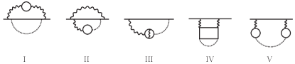
Figure 1: The different sets of vacuum polarization diagrams and light-by-light diagrams (set IV). Each set represents the drawn diagram plus all the possible permutations of its pieces.

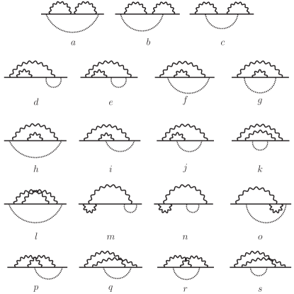
Figure 2: The diagrams involving a two-loop electron self-interaction and vertex corrections.

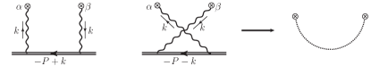
Figure 3: The sum of the direct and crossed diagrams is represented by a dotted line (the double line represents the propagator of the muon).

In order to evaluate the loop integrals represented by the Feynman diagrams we use the method of regions Smirnov:2002pj to construct an expansion in the small ratio $m/M$. There are several possible contributing regions, where one or more of the loop momenta scale like $m$ or $M$. However, we are only interested in the leading order in $m/M$, which is given by the region where all loop momenta scale like $m$. If $k\sim m$, we can expand the contribution from the muon line in the sum of the direct and crossed diagrams of Fig. 3,

$$\gamma_{\alpha}\frac{\not{k}-\not{P}+M}{(k-P)^{2}-M^{2}+i\epsilon}\gamma_{\beta}-\gamma_{\beta}\frac{\not{k}+\not{P}-M}{(k+P)^{2}-M^{2}+i\epsilon}\gamma_{\alpha}$$

$$\to T_{1}+T_{2}+T_{3}\,,$$ (9)

where

$$T_{1}= 2P_{\beta}\gamma_{\alpha}\left[\left(\frac{1}{2P\cdot k-i\epsilon}-\frac{1}{2P\cdot k+i\epsilon}\right)+\mathcal{O}\left(\frac{1}{P^{2}}\right)\right]\,,$$ (10)

$$T_{2}= -\gamma_{\alpha}\not{k}\gamma_{\beta}\left[\left(\frac{1}{2P\cdot k-i\epsilon}-\frac{1}{2P\cdot k+i\epsilon}\right)+\mathcal{O}\left(\frac{1}{P^{2}}\right)\right]\,,$$ (11)

$$T_{3}= -\left(\gamma_{\alpha}\not{k}\gamma_{\beta}+\gamma_{\beta}\not{k}\gamma_{\alpha}\right)\left[\frac{1}{2P\cdot k+i\epsilon}+\mathcal{O}\left(\frac{1}{P^{2}}\right)\right]\,.$$ (12)

We used the equation of motion to set some terms in the numerator to zero, and we arranged the terms in the expansion in such a way that the three different Dirac structures that are important for the calculation of the hyperfine splitting appear explicitly. We will now see that only $T_{2}$ can contribute to the splitting.

Consider the Dirac structure of $\psi T_{1}$ and anticommute the gamma matrices, for both para and ortho states:

$$\chi^{para}_{T_{1}} \equiv \frac{1+\gamma_{0}}{2\sqrt{2}}\gamma_{5}\,\gamma_{\alpha}$$ (13)

$$= -\gamma_{\alpha}\frac{1-\gamma_{0}}{2\sqrt{2}}\gamma_{5}-\frac{1}{\sqrt{2}}g_{\alpha 0}\gamma_{5}\,,$$

$$\chi^{ortho}_{T_{1}} \equiv \frac{1+\gamma_{0}}{2\sqrt{2}}\gamma_{i}\,\gamma_{\alpha}$$

$$= -\gamma_{\alpha}\frac{1-\gamma_{0}}{2\sqrt{2}}\gamma_{i}-\frac{1}{\sqrt{2}}g_{\alpha 0}\gamma_{i}+\frac{1}{\sqrt{2}}g_{\alpha i}(1+\gamma_{0})\,.$$

Now we can write

$$i\mathcal{M}_{T_{1}} \equiv -\text{Tr}\{\psi^{\dagger}\mathcal{Q}_{1}\psi T_{1}\}$$ (15)

$$\propto \text{Tr}\{\psi^{\dagger}\mathcal{Q}_{1}\chi_{T_{1}}\}=\text{Tr}\{\chi_{T_{1}}\psi^{\dagger}\mathcal{Q}_{1}\}\,.$$

Using the expressions in Eqs. (13) and (II) it is easy to see that $\chi^{para}_{T_{1}}\psi_{para}^{\dagger}=\chi^{ortho}_{T_{1}}\psi_{ortho}^{\dagger}$ (after averaging over polarizations). This means that $T_{1}$ gives the same contribution for para and ortho states. Therefore, when we subtract these contributions in order to compute the hyperfine splitting, they cancel out.

If we consider $T_{2}$ instead, defining $\chi_{T_{2}}$ in analogy with Eqs. (13) and (II), we can see that $\chi^{para}_{T_{2}}\psi_{para}^{\dagger}\neq\chi^{ortho}_{T_{2}}\psi_{ortho}^{\dagger}$, so this term will not cancel in the subtraction. The difference between the para and ortho states comes solely from terms in $\chi^{ortho}_{T_{2}}$ that are totally antisymmetric in $\alpha$ and $\beta$. Therefore, when we consider the Dirac structure of $T_{3}$, which is but a symmetrization of that of $T_{2}$, these terms will vanish, and so $T_{3}$ will give no contribution to the hyperfine splitting either.

Thus, we have seen that the only term that contributes to the hyperfine splitting is

$$-\gamma_{\alpha}\not{k}\gamma_{\beta}\left[\left(\frac{1}{2P\cdot k-i\epsilon}-\frac{1}{2P\cdot k+i\epsilon}\right)+\mathcal{O}\left(\frac{1}{P^{2}}\right)\right]\,.$$ (16)

This is valid at all orders of alpha, and all orders in $m/M$. We can then substitute the scalar part of the nucleon propagator by a Dirac delta in all our calculations, since we are only interested in the leading order in $m/M$ and

$$\frac{1}{2P\cdot k-i\epsilon}-\frac{1}{2P\cdot k+i\epsilon}=i\pi\delta\left(P\cdot k\right)\,.$$ (17)

We used dimensional regularization, and renormalized our results using the on-shell renormalization scheme. For all the photon propagators in Figs. 1 and 2 we used a general covariant $R_{\xi}$ gauge. The overall cancellation of the dependence on the gauge parameter in the final result provides us with a good check for our calculations.

We used the program qgraf Nogueira:1991ex to generate all of the diagrams, and the packages q2e and exp Harlander:1997zb ; Seidensticker:1999bb to express them as a series of vertices and propagators that can be read by the FORM Vermaseren:2000nd package MATAD 3 Steinhauser:2000ry . Finally, MATAD 3 was used to represent the diagrams in terms of a set of scalar integrals using custom-made routines. In this way, we represented the amplitude $\mathcal{M}$ in terms of several thousand different scalar integrals. These integrals can be expressed in terms of a few master integrals by means of integration-by-parts (IBP) identities Chetyrkin:1981qh . We used the so-called Laporta algorithm Laporta:1996mq ; Laporta:2001dd as implemented in the Mathematica package FIRE Smirnov:2008iw , to reduce the problem to 32 master integrals. The master integrals for this calculation are the same ones we found in Dowling:2009md . All definitions and results for the integrals can be found in this reference. However, one change was made for this calculation. In order to obtain better numerical precision, we performed a change of basis, so that instead of working with $I_{14}=F(1,0,0,0,1,1,1,1)$ we worked with

$$F(1,0,0,0,1,1,1,2)$$ (18)

$$= 44.55822275(2)-427.382296(2)\epsilon+\mathcal{O}(\epsilon^{2})\,,$$

which was obtained using the Mathematica package FIESTA 1.2.1 Smirnov:2008py with integrators from the CUBA library Hahn:2004fe .

III Results

Our final result for the hyperfine splitting is

$$\delta E_{hfs}=0.77099(2)\cdot\frac{\alpha^{2}(Z\alpha)}{\pi n^{3}}E_{F}\,.$$ (19)

This correction was also found by Eides and Shelyuto Eides:1995ey , and by Kinoshita and Nio Kinoshita:1995mt . Their results are

$$\delta E_{hfs} = 0.7716(4)\cdot\frac{\alpha^{2}(Z\alpha)}{\pi n^{3}}E_{F}\quad\,\,\,\text{\cite[cite]{\@@bibref{Authors Phrase1YearPhrase2}{Eides:1995ey}{\@@citephrase{(}}{\@@citephrase{)}}}}\,,$$ (20)

$$\delta E_{hfs} = 0.7679(79)\cdot\frac{\alpha^{2}(Z\alpha)}{\pi n^{3}}E_{F}\quad\text{\cite[cite]{\@@bibref{Authors Phrase1YearPhrase2}{Kinoshita:1995mt}{\@@citephrase{(}}{\@@citephrase{)}}}}\,.$$ (21)

Our result is a little over one order of magnitude more precise than that of Eides:1995ey , and almost three orders of magnitude more precise than the one in Kinoshita:1995mt . Our central value is slightly lower than in Eides:1995ey , by about $1.5\sigma$ (taking as $\sigma$ the larger error). It agrees with the result of Kinoshita:1995mt within its much larger error estimate. For the ground state of muonium, our result reads

$$\delta E_{hfs}=0.42524(1)\,\text{kHz}\,.$$ (22)

We compared our results for the individual diagrams and those found in the literature EKS2 ; EKS2b ; EKS3 ; Eides:1995ey ; Kinoshita:1995mt . Our results for the gauge-invariant sets of diagrams of Fig. 1 are presented in Table 1. For the diagrams of Fig. 2 we chose the Fried-Yennie gauge Fried:1958zz ; Adkins:1993qm , in which all diagrams are infrared finite. Our results are presented in Table 2.

Table 1: Comparison between our results for sets of diagrams of Fig. 1 and those of EKS2 ; EKS2b ; EKS3 . Numbers ending in an ellipsis indicate an analytic result, which we show in Appendix A. No error was given for the numerical result of set I in EKS2b .

Set	This paper	Refs. EKS2 ; EKS2b ; EKS3
I	$-0.31074204276602(3)$	$-0.310742$
II	$-0.668915\dots$	$-0.668915\dots$
III	$1.867852\dots$	$1.867852\dots$
IV	$-0.4725146(2)$	$-0.472514(1)$
V	$36/35$	$36/35$

Table 2: Comparison between our results for diagrams $a$–$s$ (in Fried-Yennie gauge) and those of Eides:1995ey .

Diagram	This paper	Ref. Eides:1995ey
$a$	$9/4$	$9/4$
$b$	$-6.6602948853575169751(3)$	$-6.65997(1)$
$c$	$3.9324055550472089860(4)$	$3.93208(1)$
$d$	$-3.9032816968990(2)$	$-3.903368(79)$
$e$	$4.5667195410288(2)$	$4.566710(24)$
$f$	$-3\pi^{2}/8+19/64$	$-3.404163(22)$
$g$	$\pi^{2}/2-9/4$	$2.684706(26)$
$h$	$33/16$	$33/16$
$i$	$0.05454(1)$	$0.054645(46)$
$j$	$-7.14963(2)$	$-7.14937(16)$
$k$	$1.4658690989997(5)$	$1.465834(20)$
$l$	$-1.98334(3)$	$-1.983298(95)$
$m$	$3.16949(2)$	$3.16956(16)$
$n$	$-3.59661163(2)$	$-3.59566(14)$
$o$	$1.80476(5)$	$1.804775(46)$
$p$	$3.507035(6)$	$3.50608(16)$
$q$	$-0.80380(3)$	$-0.80380(15)$
$r$	$1.05247(3)$	$1.05298(18)$
$s$	$0.277336777308(2)$	$0.277203(27)$

The sum of all central values in the second column of Tables 1 and 2 gives the coefficient $0.77099$ in Eq. (19). The error of that result is however not obtained from the sum of the errors of the diagrams in the tables. Once we decompose the problem into the calculation of master integrals, the diagrams are no longer independent, as the same master integral contributes to several different diagrams. Thus, to find the error of our total result, we first sum all diagrams and then sum all the errors of the integrals in quadrature.

We found new analytic results for diagrams $g$ and $f$, shown in Table 2. For completeness, the known analytic results for sets II and III of the vacuum polarization diagrams are given in Appendix A as well.

We found no discrepancies between our results for the diagrams of Fig. 1 and the ones of EKS2 ; EKS2b ; EKS3 , but we found significant differences in the rest of the diagrams between the results of Eides:1995ey and ours. They affect all diagrams except diagrams $a$, $e$, $h$, $l$, $o$, and $q$. The biggest discrepancies are in diagrams $b$ and $c$, and they are of the order of $30\sigma$. However, most of the differences cancel when summing the diagrams. In particular, there are almost exact cancellations between the differences in diagrams $b$ and $c$, $k$ and $l$, and $n$ and $p$.

The reason for the discrepancies (and their cancellations) is most likely the different treatment of infrared divergences in Eides:1995ey and this paper. In Eides:1995ey , the Fried-Yennie gauge was set from the beginning, and all spurious infrared divergences were canceled before the integration over the diagram’s loop momenta, which was performed in four dimensions. In our calculation, we used a general gauge parameter, and dimensional regularization to deal with infrared divergences, which would only vanish after setting the gauge in the final expression. As noted in Tomozawa:1979xn , there is a difference between setting the Fried-Yennie gauge and sending the infrared regulator to zero before or after integration. It is not surprising then that we obtained different results than Eides:1995ey for gauge-dependent diagrams, but that most of the differences cancel in the final, gauge-invariant result, making it compatible with the previous calculation.

Using the setup of the calculation of the hyperfine splitting one can also find the Lamb shift, as it is given by

$$\delta E_{Lamb}=\frac{\delta E_{ortho}\,(d-1)+\delta E_{para}}{d}\,.$$ (23)

We obtained in this way the same results as in Dowling:2009md .

Appendix A Analytic results

Here we show the analytic results for sets II and III of the vacuum polarization diagrams, found in EKS2 ,

Set II $$= -\frac{4}{3}\ln^{2}\left(\frac{1+\sqrt{5}}{2}\right)-\frac{20}{9}\sqrt{5}\,\text{ln}\left(\frac{1+\sqrt{5}}{2}\right)$$ (24)

$$-\frac{64}{45}\ln 2+\frac{\pi^{2}}{9}+\frac{10369}{5400}\,,$$

Set III $$= \frac{224}{15}\ln 2-\frac{38}{15}\pi-\frac{118}{225}\,.$$ (25)

References

- (1) P. J. Mohr, B. N. Taylor and D. B. Newell, Rev. Mod. Phys. 80, 633 (2008) [arXiv:0801.0028 [physics.atom-ph]].
- (2) B. L. Roberts, arXiv:1001.2898 [hep-ex].
- (3) M. I. Eides, H. Grotch and V. A. Shelyuto, Phys. Rept. 342, 63 (2001) [arXiv:hep-ph/0002158].
- (4) M. I. Eides, H. Grotch and V. A. Shelyuto, Theory of Light Hydrogenic Bound States, Springer Tracts Mod. Phys. 222, 1 (2007).
- (5) M. I. Eides and V. A. Shelyuto, Phys. Rev. Lett. 103, 133003 (2009) [arXiv:0907.1923 [hep-ph]].
- (6) M. I. Eides and V. A. Shelyuto, Phys. Rev. A 52, 954 (1995) [arXiv:hep-ph/9501303].
- (7) T. Kinoshita and M. Nio, Phys. Rev. D 53, 4909 (1996) [arXiv:hep-ph/9512327].
- (8) A. Czarnecki, K. Melnikov and A. Yelkhovsky, Phys. Rev. Lett. 82, 311 (1999) [arXiv:hep-ph/9809341].
- (9) V. A. Smirnov, Applied Asymptotic Expansions in Momenta and Masses, Springer Tracts Mod. Phys. 177, 1 (2002).
- (10) P. Nogueira, J. Comput. Phys. 105, 279 (1993).
- (11) R. Harlander, T. Seidensticker and M. Steinhauser, Phys. Lett. B 426, 125 (1998) [arXiv:hep-ph/9712228].
- (12) T. Seidensticker, arXiv:hep-ph/9905298.
- (13) J. A. M. Vermaseren, arXiv:math-ph/0010025.
- (14) M. Steinhauser, Comput. Phys. Commun. 134, 335 (2001) [arXiv:hep-ph/0009029]; URL: http://www-ttp.particle.uni-karlsruhe.de/~ms/software.html.
- (15) F. V. Tkachov, Phys. Lett. B 100, 65 (1981); K. G. Chetyrkin and F. V. Tkachov, Nucl. Phys. B 192, 159 (1981).
- (16) S. Laporta and E. Remiddi, Phys. Lett. B 379, 283 (1996) [arXiv:hep-ph/9602417].
- (17) S. Laporta, Int. J. Mod. Phys. A 15, 5087 (2000) [arXiv:hep-ph/0102033].
- (18) A. V. Smirnov, JHEP 0810, 107 (2008) [arXiv:0807.3243 [hep-ph]].
- (19) M. Dowling, J. Mondejar, J. H. Piclum and A. Czarnecki, Phys. Rev. A 81, 022509 (2010) [arXiv:0911.4078 [hep-ph]].
- (20) A. V. Smirnov and M. N. Tentyukov, Comput. Phys. Commun. 180, 735 (2009) [arXiv:0807.4129 [hep-ph]].
- (21) T. Hahn, Comput. Phys. Commun. 168, 78 (2005) [arXiv:hep-ph/0404043].
- (22) M. I. Eides, S. G. Karshenboim, and V. A. Shelyuto, Phys. Lett. B 229, 285 (1989).
- (23) M. I. Eides, S. G. Karshenboim, and V. A. Shelyuto, Phys. Lett. B 249, 519 (1990).
- (24) M. I. Eides, S. G. Karshenboim, and V. A. Shelyuto, Yad. Fiz. 55, 466 (1992) [Eng. transl.: Sov. J. Nucl. Phys. 55, 257 (1992)]; Phys. Lett. B 268, 433 (1991); Phys. Lett. B 316, 631(E) (1993); Phys. Lett. B 319, 545(E) (1993).
- (25) H. M. Fried and D. R. Yennie, Phys. Rev. 112, 1391 (1958).
- (26) G. S. Adkins, Phys. Rev. D 47, 3647 (1993).
- (27) Y. Tomozawa, Annals Phys. 128, 491 (1980).
- (28) J. A. M. Vermaseren, Comput. Phys. Commun. 83, 45 (1994).
- (29) D. Binosi, J. Collins, C. Kaufhold and L. Theussl, Comput. Phys. Commun. 180, 1709 (2009) [arXiv:0811.4113 [hep-ph]].