Lattice Green’s function for crystals containing a planar interface

Abstract

Flexible boundary condition methods couple an isolated defect to a harmonically responding medium through the bulk lattice Green’s function; in the case of an interface, interfacial lattice Green’s functions. We present a method to compute the lattice Green’s function for a planar interface with arbitrary atomic interactions suited for the study of line defect/interface interactions. The interface is coupled to two different semi-infinite bulk regions, and the Green’s function for interface-interface, bulk-interface and bulk-bulk interactions are computed individually. The elastic bicrystal Green’s function and the bulk lattice Green’s function give the interaction between bulk regions. We make use of partial Fourier transforms to treat in-plane periodicity. Direct inversion of the force constant matrix in the partial Fourier space provides the interface terms. The general method makes no assumptions about the atomic interactions or crystal orientations. We simulate a screw dislocation interacting with a $(10\bar{1}2)$ twin boundary in Ti using flexible boundary conditions and compare with traditional fixed boundary conditions results. Flexible boundary conditions give the correct core structure with significantly less atoms required to relax by energy minimization. This highlights the applicability of flexible boundary conditions methods to modeling defect/interface interactions by ab initio methods.

I Introduction

Accurate atomic scale studies of lattice defect geometry is the key to any modeling of their effects on material properties. However, the long-range (elastic) displacement field of isolated defects, e.g., dislocations, is incompatible with periodic boundary conditions typically used in computer atomistic simulations. Fixed boundary conditions require simulation sizes large enough for the elastic solution to be accurate—a size typically beyond even modern density-functional theory methods. Flexible boundary condition methods avoid these issues by relaxing the atoms away from the defect core through lattice Green’s function (LGF) as if they are embedded in an infinite harmonic medium. Hence, the atomic scale geometry of the defect core is coupled to the long-range strain field in the surrounding medium. Sinclair et al. introduced flexible boundary conditions for studying defects in bulk materialsref:Sinclair such as cracksThomson:rel ; crack , dislocationsRao-dislocation ; Rao-screw ; Yang-screw ; Rao-slip , vacancies with classical potentials and isolated screw or edge dislocations with density-functional theoryRao-screw-DFT ; ref:woodward ; ww-screw-DFT ; al-prl . Flexible boundary conditions use the LGF corresponding to the specific geometry of the problem. For instance, line defects in the presence of interfaces require the interfacial lattice Green’s function (ILGF). Line defects in interfaces affect the mechanical properties of composites, two-phase or polycrystalline materials where heterophase or homophase interfaces interact with defects. Tewary and Thomsonref:tewary_lgf proposed a Dyson-equation calculation of the interfacial lattice Green’s function suitable for materials with short-range atomic interactions and simple crystal structures. We present a general—for all types of interactions and interface orientations—accurate method to compute the interfacial lattice Green’s function, suited to use in density functional theory. Specifically, this method is applicable to studies of line defects interactions with planar interfaces such as disconnections in interfaces and dislocation or crack tips interacting with grain boundaries and two-phase interfaces. We compute the Green’s function for a $\left(10\bar{1}2\right)$ twin boundary in Ti to simulate a screw dislocation interacting with the twin boundary using flexible boundary conditions. Section II reviews the harmonic response functions: the force constant matrix and the lattice Green’s function. Section III explains the general procedure for evaluation of the interfacial lattice Green’s function and section IV applies the method to modeling the interaction of a screw dislocation with Ti $\left(10\bar{1}2\right)$ twin boundary. The end result is a computationally tractable, general approach usable for studies of defects in interfaces.

II Harmonic Response

Harmonic response is characterized by a linear relationship between forces and displacementsref:harmonic . Lattice Green’s function $\underline{G}(\vec{R},\vec{R}^{\prime})$ relates the displacement $\vec{u}(\vec{R})$ of atom $\vec{R}$ to the internal forces $\vec{f}(\vec{R}^{\prime})$ on another atom $\vec{R}^{\prime}$ of the crystal through

$$\vec{u}(\vec{R})=-\sum_{\vec{R}^{\prime}}\underline{G}(\vec{R},\vec{R}^{\prime})\vec{f}(\vec{R}^{\prime}).$$ (1)

Conversely, the forces on an atom can be expressed in terms of displacements through the force constant matrix $\underline{D}(\vec{R},\vec{R}^{\prime})$ by

$$\vec{f}(\vec{R})=-\sum_{\vec{R}^{\prime}}\underline{D}(\vec{R},\vec{R}^{\prime})\vec{u}(\vec{R}^{\prime}).$$ (2)

Translational invariance of an infinite crystal makes $\underline{G}$ and $\underline{D}$ functions of the relative positions of the atoms. Substituting Eqn. (2) into Eqn. (1) gives $\displaystyle\sum_{\vec{R}^{\prime}}\underline{G}(\vec{R}-\vec{R}^{\prime})\underline{D}(\vec{R}^{\prime})=\textbf{1}\delta(\vec{R})$, where $\delta(\vec{R})$ is the Kronecker delta function. A constant shift in atom positions does not produce internal forces; hence, $\sum_{\vec{R}}{\underline{D}(\vec{R})}=0$, and so $\underline{G}(\vec{R})$ is the pseudo inverse of $\underline{D}(\vec{R})$ in the subspace without uniform displacements or forces. In a bulk geometry, the Fourier transform of the lattice functions are defined as

$$\utilde{G}(\vec{k})=\sum_{\vec{R}}e^{i\vec{k}\cdot\vec{R}}\underline{G}(\vec{R}),\quad\underline{G}(\vec{R})=\int_{BZ}\frac{d^{3}k}{(2\pi)^{3}}e^{-i\vec{k}\cdot\vec{R}}\utilde{G}(\vec{k})$$

where the summation is over lattice points. In reciprocal space, the matrix inverse relation $\utilde{G}(\vec{k})\utilde{D}(\vec{k})=1$ and the sum rule $\utilde{D}(\vec{0})=0$ require that $\utilde{G}(\vec{k})$ has a pole at the $\Gamma$-point. While computation of the force constant matrix $\underline{D}(\vec{R})$—and subsequently $\utilde{D}(\vec{k})$—is straightforward, $\underline{G}(\vec{R})$ can not be computed directly due to its long range behavior. Instead, we invert $\utilde{D}(\vec{k})$ to get $\utilde{G}(\vec{k})$ and then perform an inverse Fourier transform. Convergence of the inverse Fourier transform requires an analytical treatment of the pole at the $\Gamma$-pointref:lgf ; ref:effic . In an interface geometry, translational invariance is broken in the direction perpendicular to the interface; we use Fourier transforms in the interface plane only. This produces an infinite dimensional dynamical matrix that can not be simply inverted, but requires a more complex computational approach.

III Computation of lattice Green’s function for a planar interface

Figure 1a shows two lattices, $\lambda$ and $\mu$ joined at a planar interface. Each set of vectors $\vec{a_{1}}^{\lambda,\mu}$, $\vec{a_{2}}^{\lambda,\mu}$ and $\vec{a_{3}}^{\lambda,\mu}$ give the periodic directions in their corresponding lattice. We introduce integer matrices $\underline{M}^{\lambda}$ and $\underline{M}^{\mu}$ and deformation operators $\underline{F}^{\lambda}$ and $\underline{F}^{\mu}$ so that

$$\underline{F}^{\lambda,\mu}\left[\vec{a_{1}}^{\lambda,\mu},\vec{a_{2}}^{\lambda,\mu},\vec{a_{3}}^{\lambda,\mu}\right]\underline{M}^{\lambda,\mu}=\left[\vec{T_{1}}^{\lambda,\mu},\vec{T_{2}}^{\lambda,\mu},\vec{T_{3}}^{\lambda,\mu}\right]$$ (3)

to define the supercell. We use $\vec{T_{1}}^{\lambda}=\vec{T_{1}}^{\mu}=\vec{t}_{1}$ and $\vec{T_{2}}^{\lambda}=\vec{T_{2}}^{\mu}=\vec{t}_{2}$ as nonparallel vectors to define the interface plane where $\vec{t}_{2}$ will be the periodic threading vector for a line defect in the interface. The combined lattice has translational invariance in $\vec{t}_{1}$ and $\vec{t}_{2}$ directions in the interface plane while the periodicity is broken in directions outside the plane. Introducing a threading direction reduces the problem to 2D (i.e plain strain or anti-plane strain conditions). We confine our calculations to the plane orthogonal to $\vec{t}_{2}$ and define the Cartesian coordinate $\hat{x}$, $\hat{y}$, $\hat{z}$ so that $\vec{t}_{1}\cdot\hat{x}=a_{0}$, $\vec{t}_{2}=\left|\vec{t}_{2}\right|\hat{y}$ and $\hat{z}=\hat{x}\times\hat{y}$. Note that in general $a_{0}\neq\left|\vec{t}_{1}\right|$ because $\vec{t}_{1}$ and $\vec{t}_{2}$ can be nonorthogonal. Specifically, the lattice positions, $\vec{R}=x\hat{x}+z\hat{z}$ and the Fourier vectors, $\vec{k}=k_{x}\hat{x}+k_{z}\hat{z}$, will be 2D vectors through out this paper and

$$\underline{D}_{\alpha\alpha^{\prime}}(\vec{R},\vec{R}^{\prime})=\underline{D}_{\alpha\alpha^{\prime}}(x-x^{\prime};z,z^{\prime})$$

with $\alpha$ and $\alpha^{\prime}$ identifying the $xyz$ components of the second rank tensor $\underline{D}$ in Cartesian coordinates. We index atoms in our computational cell with integer $l$ at position $(x_{l},z_{l})$; due to periodicity in the $\hat{x}$ direction, each atom also occurs at $x_{l}+na_{0}\hat{x}$ for integer values of $n$. The partial Fourier transform is

$$\utilde{D}_{\alpha l,\alpha^{\prime}l^{\prime}}(k_{x}) = \sum_{n=-\infty}^{\infty}e^{ik_{x}(x_{l}-x_{l^{\prime}}+na_{0})}\underline{D}_{\alpha\alpha^{\prime}}(x_{l}-x_{l^{\prime}}+na_{0};z_{l},z_{l^{\prime}})$$

$$\underline{D}_{\alpha\alpha^{\prime}}(x_{l}-x_{l^{\prime}}+na_{0};z_{l},z_{l^{\prime}}) = \frac{a_{0}}{2\pi}\int_{-\pi/a_{0}}^{\pi/a_{0}}e^{-ik_{x}(x_{l}-x_{l^{\prime}}+na_{0})}\utilde{D}_{\alpha l,\alpha^{\prime}l^{\prime}}(k_{x})dk_{x}$$ (4)

for all pairs $l,l^{\prime}$. Note that “$l$” indexes layers of atoms with particular z values. There may be two different layers that have equal $z$: $z_{l}=z_{l^{\prime}}$ while $l\neq l^{\prime}$. $\utilde{D}(k_{x})$ is infinite dimensional due to infinite values of $l$.

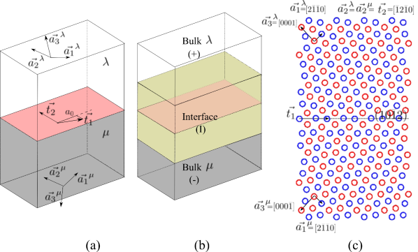
Figure 1: (a) Bicrystal $\mu$ and $\lambda$, (b) separation into bulk and interface regions and (c) the Ti $\left(10\bar{1}2\right)$ twin boundary . Two different lattices, $\lambda$ and $\mu$ are connected through a planar interface. The unit cells of $\lambda$ and $\mu$ are given by $\vec{a_{1}}^{\lambda,\mu}$,$\vec{a_{2}}^{\lambda,\mu}$ and $\vec{a_{3}}^{\lambda,\mu}$—all of which must be lattice vectors in $\lambda$ and $\mu$. The combined lattice has the periodicity of the interface in $\vec{t}_{1}$ and $\vec{t}_{2}$ directions. Introducing a line defect threading direction $\vec{t}_{2}$ reduces the problem to 2D in the plane normal to $\vec{t}_{2}$. In (b), the crystal is divided into two semi-infinite bulk regions, bulk $\lambda$ and bulk $\mu$ symbolized by $(+)$ and $(-)$ respectively, coupled with an interface region (I). The bulk regions are far from and affected only through an elastic effect by the interface. The force constant matrix between atom pairs in the bulk is not affected by the interface. The remaining layers are included in (I). (c) shows the periodicity vectors for the Ti $\left(10\bar{1}2\right)$ twin boundary. The interface is defined by $\vec{t}_{1}=\sqrt{3a^{2}+c^{2}}\hat{x}$ and $\vec{t}_{2}=a\hat{y}$ where $a$ and $c$ are the hcp unit cell parameters in Ti for both $\lambda$ and $\mu$. $\mu$ is the reflection of $\lambda$ about the interface plane.

To avoid the inversion of infinite dimensional $\utilde{D}(k_{x})$, the geometry is divided into two semi-infinite bulk regions coupled with an interface region. Figure 1b shows the schematic divisions of the regions in an interface geometry consisting of lattices $\lambda$ and $\mu$. The “bulk” regions represent layers of atoms that are far from and affected only through an elastic field by the interface. The atomic scale interaction between atom pairs are as if they were in their corresponding bulk geometry. Bulk $\lambda$ and bulk $\mu$ are symbolized by $(+)$ and $(-)$ in our notation. The remaining layers, affected by the reconstructions near the interface, are included in the “interface” region (I). We define the interface region as atoms where the force constant matrix differ from those in the bulk lattice. For specific geometries, additional bulk layers may be included in the interface to insure a smooth transition between the regions. We block partition the infinite dimensional $\utilde{D}_{\alpha l,\alpha^{\prime}l^{\prime}}(k_{x})$ and $\utilde{G}_{\alpha l,\alpha^{\prime}l^{\prime}}(k_{x})$ based on the atom region (+, $-$, or I) of indices $l$ as

$$\utilde{D}(k_{x})=\left(\begin{array}[]{c|cc}\utilde{D}^{II}(k_{x})&\utilde{D}^{I-}(k_{x})&\utilde{D}^{I+}(k_{x})\\ \hline\cr\utilde{D}^{-I}(k_{x})&\utilde{D}^{--}(k_{x})&\utilde{D}^{-+}(k_{x})\\ \utilde{D}^{+I}(k_{x})&\utilde{D}^{+-}(k_{x})&\utilde{D}^{++}(k_{x})\end{array}\right)$$ (5)

where $l>l_{+}$ belong to $(+)$ region, $l<l_{-}$ belong to $(-)$ region and the finite-dimensional region is (I). $\utilde{D}(k_{x})$ and $\utilde{G}(k_{x})$ are Hermitian and satisfy

$$\sum_{\alpha^{\prime\prime}l^{\prime\prime}}\utilde{D}_{\alpha l,\alpha^{\prime\prime}l^{\prime\prime}}(k_{x})\utilde{G}_{\alpha^{\prime\prime}l^{\prime\prime},\alpha^{\prime}l^{\prime}}(k_{x})=\delta_{\alpha\alpha^{\prime}}\delta_{ll^{\prime}}.$$ (6)

We construct $\utilde{D}(k_{x})$ by direct calculation of $\underline{D}_{\alpha\alpha^{\prime}}(x_{l}-x_{l}^{\prime}+na_{0};z_{l},z_{l}^{\prime})$ followed by a partial Fourier transform according to Eqn. (III) and block partitioning as in Eqn. (5). Note that due to the finite number of interface layers and decay of the force constant matrix, the infinite dimensional non-zero sections of $\utilde{D}(k_{x})$ consists of $--$, $-+$ and $++$ interactions (bulk-like regions with themselves) which we explicitly avoid in our approach.

The infinite dimensional blocks of $\utilde{G}(k_{x})$ are known from bicrystal elastic and bulk lattice calculations. The distance between $+$ and $-$ is large enough for the elastic Green’s function to be applicable; the real space solution of $\underline{G}^{-+}$ is calculated from the bicrystal elastic Green’s function in both plane strain and anti-plain conditions proposed by Tewary et. alref:tewary . We partially Fourier transform the real space solution by a continuum version of Eqn. (III),

$$\utilde{G}^{-+}_{\alpha l,\alpha^{\prime}l^{\prime}}(k_{x})=\int_{-\infty}^{\infty}\underline{G}^{-+}_{\alpha\alpha^{\prime}}(x;z_{l},z_{l^{\prime}})e^{ik_{x}x}dx.$$ (7)

$\utilde{G}^{+-}$ is the conjugate transpose of $\utilde{G}^{-+}$ due to $\utilde{G}(k_{x})$ being Hermitian. The functional form of $\underline{G}^{-+}(x;z_{l},z_{l^{\prime}})$ consists of real parts of $\ln(x+p^{\lambda}_{q}z_{l}+p^{\mu}_{q^{\prime}}z_{l^{\prime}})$ where $p^{\lambda}_{q}$ and $p^{\mu}_{q^{\prime}}$ are the complex roots of the sextic equation of anisotropic elasticity for bicrystal $\lambda\mu$ and $q,q^{\prime}=1,2$ in plain strain and 1 in anti-plane conditions ref:tewary . We rewrite $\ln(x+\gamma^{qq^{\prime}}_{l,l^{\prime}}+i\beta^{qq^{\prime}}_{l,l^{\prime}})$ with

$$\gamma^{qq^{\prime}}_{l,l^{\prime}}=\Re{(p^{\lambda}_{q})}z_{l}+\Re{(p^{\mu}_{q^{\prime}})}z_{l^{\prime}},\ \beta^{qq^{\prime}}_{l,l^{\prime}}=\Im{(p^{\lambda}_{q})}z_{l}+\Im{(p^{\mu}_{q^{\prime}})}z_{l^{\prime}}.$$

The Green’s function in real space is the real part of the complex logarithm with the form

$$\underline{G}^{-+}_{\alpha\alpha^{\prime}}(x;z_{l},z_{l^{\prime}})=\sum_{q,q^{\prime}}\underline{a}_{\alpha\alpha^{\prime}}^{qq^{\prime}}\ln\left|(x+\gamma^{qq^{\prime}}_{l,l^{\prime}})^{2}+(\beta^{qq^{\prime}}_{l,l^{\prime}})^{2}\right|+\underline{b}_{\alpha\alpha^{\prime}}^{qq^{\prime}}\arctan\left(\frac{\beta^{qq^{\prime}}_{l,l^{\prime}}}{x+\gamma^{qq^{\prime}}_{l,l^{\prime}}}\right)$$ (8)

where $\underline{a}_{\alpha\alpha^{\prime}}^{qq^{\prime}}$ and $\underline{b}_{\alpha\alpha^{\prime}}^{qq^{\prime}}$ are real valued coefficients of the term $qq^{\prime}.$ Eqn. (8) is obtained by rewriting Eqn. (60) in ref:tewary . The partial Fourier transform is

$$\utilde{G}_{\alpha l,\alpha^{\prime}l^{\prime}}^{-+}(k_{x})=-\frac{\pi}{\left|\vec{t}_{2}\right|\left|k_{x}\right|}\sum_{q,q^{\prime}}2\underline{a}_{\alpha\alpha^{\prime}}^{qq^{\prime}}e^{-\left|\beta^{qq^{\prime}}_{l,l^{\prime}}k_{x}\right|}e^{-i\gamma^{qq^{\prime}}_{l,l^{\prime}}k_{x}}+i\underline{b}_{\alpha\alpha^{\prime}}^{qq^{\prime}}\frac{k_{x}}{\left|k_{x}\right|}e^{-\left|\beta^{qq^{\prime}}_{l,l^{\prime}}k_{x}\right|}e^{-i\gamma^{qq^{\prime}}_{l,l^{\prime}}k_{x}}$$ (9)

with a first order pole at $k_{x}=0$. The $1/\left|\vec{t}_{2}\right|$ prefactor is required for the elastic and lattice Green’s functions to have consistent units of ($\text{length}^{2}/\text{energy}$). We separate the pole from the remainder of the Green’s function

$$\utilde{G}^{-+}_{\alpha l,\alpha^{\prime}l^{\prime}}(k_{x})=\frac{\hat{\utilde{G}}_{\alpha\alpha^{\prime}}^{-+}}{\left|k_{x}\right|}+\check{\utilde{G}}_{\alpha l,\alpha^{\prime}l^{\prime}}^{-+}(k_{x}).$$ (10)

The pole with a constant coefficient $\hat{\utilde{G}}^{-+}_{\alpha\alpha^{\prime}}=-\frac{\pi}{\left|\vec{t}_{2}\right|}\sum_{q,q^{\prime}}\underline{a}_{\alpha\alpha^{\prime}}^{qq^{\prime}}$ will be treated analytically while the nonsingular remainder $\check{\utilde{G}}^{-+}_{\alpha l,\alpha^{\prime}l^{\prime}}(k_{x})$, will be treated numerically.

The $\utilde{G}^{--}(k_{x})$ and $\utilde{G}^{++}(k_{x})$ blocks in Eqn. (5) are obtained from the bulk lattice Green’s function of $\lambda$ and $\mu$ lattices plus an elastic term due to the presence of the interface. The full Fourier transform of the bulk LGF $\utilde{G}^{\sigma\sigma}(\vec{k})$ is the inverse of the bulk dynamical matrix from Section II. The partial inverse Fourier transform gives the Green’s function in terms of $k_{x}$ and atom indices

$$\utilde{G}_{\alpha l,\alpha^{\prime}l^{\prime}}^{\sigma\sigma}(k_{x})=\frac{1}{A_{BZ}}\int_{k_{i}(k_{x})}^{k_{f}(k_{x})}\utilde{G}_{\alpha\alpha^{\prime}}^{\sigma\sigma}(\vec{k})e^{-ik_{z}(z_{l}-z_{l^{\prime}})}dk_{z}$$ (11)

for $\vec{k}=(k_{x}\hat{x},k_{z}\hat{z})$ in the Brillouin zone (BZ), $A_{BZ}$ the area of the BZ and $k_{i}(k_{x})$ and $k_{f}(k_{x})$ showing the initial and final values of $k_{z}$ at each $k_{x}$. $\utilde{G}_{\alpha\alpha^{\prime}}^{\sigma\sigma}(\vec{k})$ has a second order pole at $k=\sqrt{k_{x}^{2}+k_{z}^{2}}=0$ which is responsible for the logarithmic long range behavior of LGF in real space. The LGF in reciprocal space is

$$\utilde{G}^{\sigma\sigma}_{\alpha\alpha^{\prime}}(\vec{k})=\frac{\hat{\utilde{G}}_{\alpha\alpha^{\prime}}^{\sigma\sigma}(\hat{k})}{k_{x}^{2}+k_{z}^{2}}f_{c}(k)+\check{\utilde{G}}_{\alpha\alpha^{\prime}}^{\sigma\sigma}(\vec{k})$$

where $\hat{\utilde{G}}^{\sigma\sigma}$ is the $\hat{k}$ direction-dependent elastic Green’s function and $f_{c}(k)$ is a cutoff function that vanishes smoothly at the edges of the BZ. In general anisotropic cases, $\hat{\utilde{G}}^{\sigma\sigma}(\hat{k})$ is represented by a Fourier series expansion as $\hat{\utilde{G}}_{\alpha\alpha^{\prime}}^{\sigma\sigma}(\hat{k})=\displaystyle\sum_{n=0}^{N_{\text{max}}}\hat{\utilde{G}}_{\alpha\alpha^{\prime}}^{\sigma\sigma,n}e^{in\phi_{k}}$ where $\phi_{k}$ is the angle of $\vec{k}$ relative to an arbitrary in-plane direction and the truncation $N_{\text{max}}$ is sufficiently largeref:lgf . The integrand in Eqn. (11) is not singular for $k_{x}\neq 0$ however the $k^{2}$ pole in $\utilde{G}^{\sigma\sigma}(\vec{k})$ results in a pole of order $\left|k_{x}\right|$ in $\utilde{G}_{\alpha l,\alpha^{\prime}l^{\prime}}^{\sigma\sigma}(k_{x})$. To treat the small $k_{x}$ behavior analytically, we integrate Eqn. (11) as four terms

$$\int_{k_{i}(k_{x})}^{k_{f}(k_{x})}\utilde{G}_{\alpha\alpha^{\prime}}^{\sigma\sigma}(\vec{k})e^{-ik_{z}(z_{l}-z_{l^{\prime}})}dk_{z} = \int_{k_{i}(k_{x})}^{k_{f}(k_{x})}\utilde{G}_{\alpha\alpha^{\prime}}^{\sigma\sigma}(\vec{k})(e^{-ik_{z}(z_{l}-z_{l^{\prime}})}-1)dk_{z}$$

$$+ \int_{k_{i}(k_{x})}^{k_{f}(k_{x})}\utilde{G}_{\alpha\alpha^{\prime}}^{\sigma\sigma}(\vec{k})-\frac{\hat{\utilde{G}}_{\alpha\alpha^{\prime}}^{\sigma\sigma,0}}{k_{x}^{2}+k_{z}^{2}}f_{c}(k_{x},k_{z})dk_{z}$$

$$+ \int_{k_{i}(k_{x})}^{k_{f}(k_{x})}\frac{\hat{\utilde{G}}_{\alpha\alpha^{\prime}}^{\sigma\sigma,0}}{k_{x}^{2}+k_{z}^{2}}(f_{c}(k_{x},k_{z})-1)dk_{z}$$

$$+ \int_{k_{i}(k_{x})}^{k_{f}(k_{x})}\frac{\hat{\utilde{G}}_{\alpha\alpha^{\prime}}^{\sigma\sigma,0}}{k_{x}^{2}+k_{z}^{2}}dk_{z}$$

where $\hat{\utilde{G}}_{\alpha\alpha^{\prime}}^{\sigma\sigma,0}$ is the $n=0$ coefficient in Fourier expansion of $\hat{\utilde{G}}_{\alpha\alpha^{\prime}}^{\sigma\sigma}(\hat{k})$. The first three terms in Eqn. (III) are evaluated numerically while the last integral is

$$\int_{k_{i}(k_{x})}^{k_{f}(k_{x})}\frac{\hat{\utilde{G}}_{\alpha\alpha^{\prime}}^{\sigma\sigma,0}}{k_{x}^{2}+k_{z}^{2}}dk_{z}=\frac{\pi\hat{\utilde{G}}_{\alpha\alpha^{\prime}}^{\sigma\sigma,0}}{|k_{x}|}+\hat{\utilde{G}}_{\alpha\alpha^{\prime}}^{\sigma\sigma,0}\left(\frac{\arctan(k_{f}(k_{x})/k_{x})-\arctan(k_{i}(k_{x})/k_{x})}{k_{x}}-\frac{\pi}{|k_{x}|}\right)$$ (13)

where $\frac{\pi\hat{\utilde{G}}_{\alpha\alpha^{\prime}}^{\sigma\sigma,0}}{|k_{x}|}$ is the pole and the remaining terms are added to the numerically evaluated part. We add an elastic correction term to $\utilde{G}_{\alpha\alpha^{\prime}}^{\sigma\sigma}(k_{x})$, due to the interface obtained from Eqn. (59) in ref:tewary . Combining Eqn. (13), Eqn. (III), and Eqn. (10) produces

$$\utilde{G}_{\alpha l,\alpha l^{\prime}}^{\sigma\sigma^{\prime}}(k_{x})=\frac{\hat{\utilde{G}}_{\alpha\alpha^{\prime}}^{\sigma\sigma^{\prime}}}{\left|k_{x}\right|}+\check{\utilde{G}}_{\alpha l,\alpha l^{\prime}}^{\sigma\sigma^{\prime}}(k_{x}).$$ (14)

Eqn. (5) has unknown blocks $\utilde{G}^{II}(k_{x})$, $\utilde{G}^{I\sigma}(k_{x})$. Direct substitution of the block partitions gives

$$\utilde{G}^{I\sigma}(k_{x}) = -(\utilde{D}^{II}(k_{x}))^{-1}\displaystyle\sum_{\sigma^{\prime}=\pm}\utilde{D}^{I\sigma^{\prime}}(k_{x})\utilde{G}^{\sigma^{\prime}\sigma}(k_{x})$$ (15)

$$\utilde{G}^{II}(k_{x}) = (\utilde{D}^{II}(k_{x}))^{-1}+\displaystyle\sum_{\sigma^{\prime}\sigma=\pm}(\utilde{D}^{II}(k_{x}))^{-1}\utilde{D}^{I\sigma}(k_{x})\utilde{G}^{\sigma\sigma^{\prime}}(k_{x})\utilde{D}^{\sigma^{\prime}I}(k_{x})(\utilde{D}^{II}(k_{x}))^{-1}.$$ (16)

Note that by choosing the appropriate set of independent equations we manage to avoid the calculation of the infinite dimensional $\utilde{D}^{\sigma\sigma^{\prime}}(k_{x})$. The finite range of $\utilde{D}^{I\sigma}(k_{x})$ means that only a finite subset of atoms in each semi-infinite $\pm$ region are considered for $\utilde{G}^{\sigma\sigma^{\prime}}(k_{x})$. To treat the poles in $\utilde{G}^{II}(k_{x})$ and $\utilde{G}^{I\sigma}(k_{x})$ analytically, we use a $k_{x}$ expansion of $\utilde{D}(k_{x})=\hat{\utilde{D}}+\check{\utilde{D}}(k_{x})$ derived from Eqn. (III) where $\check{\utilde{D}}(k_{x})=\utilde{D}^{1}k_{x}+O(k_{x}^{2})$ . Therefore, for small $k_{x}$

$$(\utilde{D}(k_{x}))^{-1} = \left[\hat{\utilde{D}}+\check{\utilde{D}}(k_{x})\right]^{-1}$$

$$= {\hat{\utilde{D}}}^{-1}\left[\mathbf{I}+\check{\utilde{D}}(k_{x}){\hat{\utilde{D}}}^{-1}\right]^{-1}$$

$$= {\hat{\utilde{D}}}^{-1}-k_{x}{\hat{\utilde{D}}}^{-1}\utilde{D}^{1}{\hat{\utilde{D}}}^{-1}+O(k_{x}^{2}).$$

Using the small $k_{x}$ expansions for the bulk Green’s functions with Eqn. (15) and Eqn. (16) gives

$$\utilde{G}^{I\sigma}(k_{x})=\frac{1}{\left|k_{x}\right|}\hat{\utilde{G}}^{I\sigma}+\check{\utilde{G}}^{I\sigma}(k_{x})\ \text{and}\ \utilde{G}^{II}(k_{x})=\frac{1}{\left|k_{x}\right|}\hat{\utilde{G}}^{II}+\check{\utilde{G}}^{II}(k_{x})$$ (18)

where

$$\hat{\utilde{G}}^{I\sigma}=-(\hat{\utilde{D}}^{II})^{-1}\sum_{\sigma^{\prime}=\pm}\hat{\utilde{D}}^{I\sigma^{\prime}}\hat{\utilde{G}}^{\sigma^{\prime}\sigma}\text{ and }\hat{\utilde{G}}^{II}=(\hat{\utilde{D}}^{II})^{-1}+\sum_{\sigma,\sigma^{\prime}=\pm}(\hat{\utilde{D}}^{II})^{-1}\hat{\utilde{D}}^{I\sigma}\hat{\utilde{G}}^{\sigma\sigma^{\prime}}\hat{\utilde{D}}^{\sigma^{\prime}I}(\hat{\utilde{D}}^{II})^{-1}$$

are the constant coefficients of the pole and $\check{\utilde{G}}^{I\sigma}(k_{x})$ and $\check{\utilde{G}}^{II}(k_{x})$ include the remaining nonsingular terms. $\check{\utilde{G}}^{II}(k_{x})$ and $\check{\utilde{G}}^{I\sigma}(k_{x})$ have a cusp approaching $k_{x}=0$ and the value at $k_{x}=0$ is

$$\check{\utilde{G}}^{I\sigma}(0) = -(\hat{\utilde{D}}^{II})^{-1}\sum_{\sigma^{\prime}=\pm}\hat{\utilde{D}}^{I\sigma^{\prime}}\check{\utilde{G}}^{\sigma^{\prime}\sigma}(0)$$ (19)

$$\check{\utilde{G}}^{II}(0) = (\hat{\utilde{D}}^{II})^{-1}+\sum_{\sigma,\sigma^{\prime}=\pm}(\hat{\utilde{D}}^{II})^{-1}\hat{\utilde{D}}^{I\sigma}\check{\utilde{G}}^{\sigma\sigma^{\prime}}(0)\hat{\utilde{D}}^{\sigma^{\prime}I}(\hat{\utilde{D}}^{II})^{-1}$$ (20)

where $\check{\utilde{G}}^{\sigma\sigma^{\prime}}(0)$ is calculated in Appendix A. To ensure a smooth transition between interface and bulk regions, we compare the pole terms and the cusps for atom indices at the boundary between the regions (i.e $l_{+}$ and $l_{-}$). Labeling $l_{\sigma}$ as $\sigma=\pm$ or (I) does not change the material response. Specifically we should have

$$\hat{\utilde{G}}_{\alpha l_{\sigma},\alpha^{\prime}l_{\sigma}}^{II}=\hat{\utilde{G}}_{\alpha\alpha^{\prime}}^{\sigma\sigma} \check{\utilde{G}}_{\alpha l_{\sigma},\alpha^{\prime}l_{\sigma}}^{II}(0)=\check{\utilde{G}}_{\alpha l_{\sigma},\alpha^{\prime}l_{\sigma}}^{\sigma\sigma}(0)$$ , (21)

Eqn. (21) determines the finite size effect in the interface. Note that once the bulk force constant matrix is known, identifying atoms in the interface region does not require additional computation effort.

Evaluating the Green’s function in real space between to atoms $(x_{l}+na_{0},z_{l})$ and $(x_{l^{\prime}},z_{l^{\prime}})$ requires a partial inverse Fourier transform over Eqn. (18),

$$\underline{G}_{\alpha\alpha^{\prime}}^{I\sigma}(x_{l}-x_{l^{\prime}}+na_{0};z_{l},z_{l^{\prime}})=\int_{-k_{\text{max}}}^{k_{\text{max}}}\utilde{G}_{\alpha l,\alpha^{\prime}l^{\prime}}^{I\sigma}(k_{x})e^{-ik_{x}(x_{l}-x_{l^{\prime}}+na_{0})}dk_{x}$$ (22)

and

$$\underline{G}_{\alpha\alpha^{\prime}}^{II}(x_{l}-x_{l^{\prime}}+na_{0};z_{l},z_{l^{\prime}})=\int_{-k_{\text{max}}}^{k_{\text{max}}}\utilde{G}_{\alpha l,\alpha^{\prime}l^{\prime}}^{II}(k_{x})e^{-ik_{x}(x_{l}-x_{l^{\prime}}+na_{0})}dk_{x}.$$ (23)

The $\hat{\utilde{G}}$ term in Eqn. (18) is treated analytically via

$$\int_{-\infty}^{\infty}\frac{1}{\left|k_{x}\right|}e^{-ik_{x}x}dk_{x}=-2\ln\left|x\right|.$$

Therefore

$$\int_{-k_{\text{max}}}^{k_{\text{max}}}{\frac{1}{|k_{x}|}e^{-ik_{x}x}}dk_{x}=-2\ln|x|+2\text{Ci}(k_{\text{max}}x).$$ (24)

Note that $\lim\limits_{x\to 0}-2\ln|x|+2\text{Ci}=2\gamma+2\ln(k_{\text{max}})$ where $\gamma\approx 0.577215$ is the Euler constant. The partial inverse Fourier transform for $\check{\utilde{G}}$ terms are evaluated numerically over a discrete $k_{x}$ mesh of size $N_{k_{x}}$

$$\check{\utilde{G}}_{\alpha\alpha^{\prime}}^{I\sigma}(x_{l}-x_{l^{\prime}}+na_{0};z_{l},z_{l^{\prime}})=\frac{1}{N_{k_{x}}}\displaystyle\sum_{k_{x}}\check{\utilde{G}}_{\alpha l,\alpha^{\prime}l^{\prime}}^{I\sigma}(k_{x})e^{-ik_{x}(x_{l}-x_{l^{\prime}}+na_{0})}$$ (25)

and

$$\check{\utilde{G}}_{\alpha\alpha^{\prime}}^{II}(x_{l}-x_{l^{\prime}}+na_{0};z_{l},z_{l^{\prime}})=\frac{1}{N_{k_{x}}}\displaystyle\sum_{k_{x}}\check{\utilde{G}}_{\alpha l,\alpha^{\prime}l^{\prime}}^{II}(k_{x})e^{-ik_{x}(x_{l}-x_{l^{\prime}}+na_{0})}.$$ (26)

Table 1 summarizes the method.

Table 1: Summary of the procedure for ILGF computation. Regions (+, $-$, and I) are defined in Figure 1b. $\underline{G}^{\--+}(x;z,z^{\prime})$ is the elastic Green’s function for a bicrystal computed by Tewary et al.ref:tewary . $\utilde{G}^{\sigma\sigma}(\vec{k})$ is the LGF in bulk $\sigma=\pm$. FT prefactors required to maintain the consistency between elastic bicrystal GF and bulk LGF solutions are also listed.

1. Compute $\underline{D}_{\alpha\alpha^{\prime}}(x_{l}-x_{l^{\prime}}+na_{0};z_{l},z_{l^{\prime}})$ directly. Divide the geometry into $-,\text{I},+$ regions.

2. $\utilde{D}_{\alpha l,\alpha^{\prime}l^{\prime}}^{I\sigma}(k_{x})=\displaystyle\sum_{n=-\infty}^{\infty}e^{ik_{x}(x_{l}-x_{l^{\prime}}+na_{0})}\underline{D}_{\alpha\alpha^{\prime}}^{I\sigma}(x_{l}-x_{l^{\prime}}+na_{0};z_{l},z_{l^{\prime}})$, $a_{0}=$ periodicity in $x$ direction and $\sigma=\pm,\text{I}$. Eqn. (III)

3. $\utilde{G}_{\alpha l,\alpha^{\prime}l^{\prime}}^{-+}(k_{x})=\frac{b_{1}}{2\pi\left|\vec{t}_{2}\right|}\displaystyle\int_{-\infty}^{\infty}\underline{G}_{\alpha\alpha^{\prime}}^{\--+}(x;z_{l},z_{l^{\prime}})e^{ik_{x}x}dx$, $b_{1}=\frac{2\pi}{a_{0}}$, $b_{1}b_{2}=A_{BZ}$. Eqn. (7)

4. $\utilde{G}_{\alpha l,\alpha^{\prime}l^{\prime}}^{\sigma\sigma}(k_{x})=\frac{1}{b_{2}}\displaystyle\int_{k_{i}(k_{x})}^{k_{f}(k_{x})}\utilde{G}_{\alpha\alpha^{\prime}}^{\sigma\sigma}(k_{x};k_{z})e^{-ik_{z}(z_{l}-z_{l^{\prime}})}dk_{z}$. Eqn. (11)

5. $\utilde{G}_{\alpha l,\alpha^{\prime}l^{\prime}}^{\sigma\sigma^{\prime}}(k_{x})=\frac{\hat{\utilde{G}}_{\alpha\alpha^{\prime}}^{\sigma\sigma^{\prime}}}{\left|k_{x}\right|}+\check{\utilde{G}}_{\alpha l,\alpha^{\prime}l^{\prime}}^{\sigma\sigma^{\prime}}(k_{x})$. Eqn. (14)

6. $\utilde{D}_{\alpha l,\beta n}(k_{x})\utilde{G}_{\beta n,\alpha^{\prime}l^{\prime}}(k_{x})=\delta_{\alpha\alpha^{\prime}}\delta_{ll^{\prime}}$ $\longrightarrow$ $\utilde{G}_{\alpha l,\alpha^{\prime}l^{\prime}}^{\text{I}\sigma}(k_{x})=\frac{\hat{\utilde{G}}_{\alpha\alpha^{\prime}}^{\text{I}\sigma}}{\left|k_{x}\right|}+\check{\utilde{G}}_{\alpha l,\alpha^{\prime}l^{\prime}}^{\text{I}\sigma}(k_{x})$, ($\sigma=\pm,\text{I}$). Eqn. (15)-(18)

7. $\utilde{G}_{\alpha l,\alpha^{\prime}l^{\prime}}^{I\sigma}(x=x_{l}-x_{l^{\prime}}+na_{0};z_{l},z_{l^{\prime}})$
   $=\frac{\hat{\utilde{G}}_{\alpha\alpha^{\prime}}^{\text{I}\sigma}}{b_{1}}\left(-2\ln|x|+2\text{Ci}(\frac{b_{1}}{2}x)\right)+\frac{1}{N_{k_{x}}}\!\displaystyle\sum_{m=1}^{N_{k_{x}}-1}\check{\utilde{G}}_{\alpha l,\alpha^{\prime}l^{\prime}}^{I\sigma}(\frac{mb_{1}}{N_{k_{x}}})e^{-i\frac{mb_{1}}{N_{k_{x}}}x}$. Eqn. (24)-(26)

IV Application: Lattice Green’s function for Ti $(10\bar{1}2)$ twin boundary

We use the method to compute the ILGF for a Ti lattice containing $(10\bar{1}2)$ twin boundary. The geometry of this boundary is shown in Figure 1c. The $\underline{F}^{\lambda,\mu}$ and $\underline{M}^{\lambda,\mu}$ matrices are

$$\underline{F}^{\lambda,\mu}=\mathbf{I},\ \underline{M}^{\lambda}=\left[\begin{array}[]{c c c}2&0&0\\ 1&1&0\\ 1&0&1\end{array}\right],\text{ and }\underline{M}^{\mu}=\left[\begin{array}[]{ccc}2&0&0\\ 1&1&0\\ -1&0&1\end{array}\right].$$

The twin boundary is defined by $\vec{t}_{1}=\sqrt{3a^{2}+c^{2}}\hat{x}$ and $\vec{t}_{2}=a\hat{y}$ where $a$ and $c$ are the hcp lattice constants in Ti. Lattice $\mu$ is the reflection of $\lambda$ about the twin boundary plane. The force-constant matrices $\underline{D}(\vec{R})$ are computed using lammps packageref:LAMMPS with a Ti MEAM potential with the maximum cut off distance of 5.5Åref:meam . The partial FT in Eqn. (III) is done by a uniform discrete mesh of 40 $k_{x}$ points over $(-\pi/a_{0},\pi/a_{0})$ where $a_{0}$ is the periodicity of the geometry in $x$ direction and equal to $\left|\vec{t}_{1}\right|$ in this case. The same $k_{x}$ values must be used in $(+)$,$(-)$ and (I) regions. Limits of $k_{z}$ in Eqn. (11) are then chosen so that the equivalent of $A_{BZ}$ is covered in both $(+)$ and $(-)$. The first three integrals in Eqn. (III) are evaluated numerically over a uniform $k_{z}$ mesh of 160 points at each $k_{x}$. For $\left|k_{x}\right|<0.1\pi/a_{0}$, the density of $k_{z}$ mesh is doubled to insure the convergence around the discontinuity at $\Gamma$-pointref:lgf ; ref:effic .

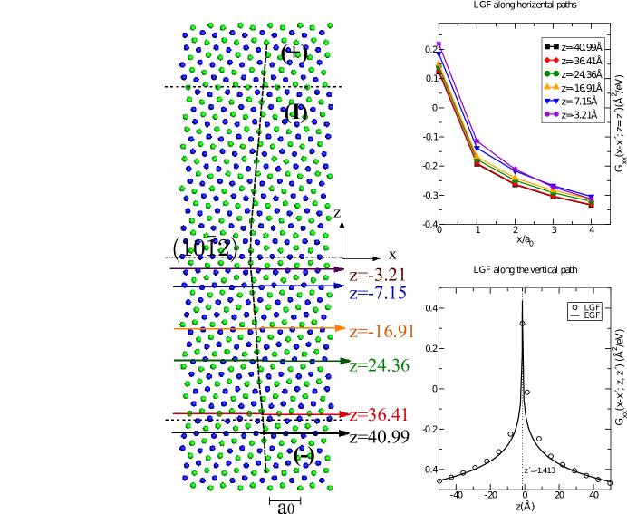
Figure 2: $\left[1\bar{2}10\right]$ projection of the Ti supercell containing a $\left(10\bar{1}2\right)$ twin boundary. The supercell is divided into bulk ($+/-$) and interface (I) regions. $y$ axis is pointing into the plane. Variation of the $G_{xx}$ component of the lattice Green’s function is plotted along six horizontal and one vertical paths. The reference atom $\left(x^{\prime},z^{\prime}\right)$ is the first atom in horizontal paths and the atom right below the interface in the vertical path. Bulk behavior along the $z=z^{\prime}$ paths is recovered away from the interface. The long range behavior of the LGF matches the EGF along the vertical path, while deviating for small $z-z^{\prime}$.

Figure 2 shows the supercell with bulk ($+/-$) and interface (I) divisions and the paths along which LGF is evaluated for testing purposes. $G_{xx}(x-x_{l^{\prime}};z_{l},z_{l^{\prime}})$ is plotted along a vertical and six horizontal paths in the supercell where the reference atom $l^{\prime}$ is the first atom ($x_{l^{\prime}}=0$) in the horizontal paths and the atom right below the interface in the vertical path. Bulk response along $z_{l}=z_{l^{\prime}}$ paths is gradually recovered as the paths get farther from the interface and closer to the ($-$) region. In addition, it is worth noting that paths 1 and 2 are located in bulk and interface regions respectively. Therefore, the LGF is obtained from the bulk lattice Green’s function along path 1 and from the ILGF method along path 2. The good agreement between the response of these two paths verifies the smooth transition between the bulk-interface divisions. $G_{xx}(x-x^{\prime};z,z^{\prime})$ as a function of $z$ is also plotted for atoms along the vertical line shown on the supercell in Figure 2. The reference atom is located on the vertical line at $x_{l^{\prime}}=x^{\prime},z_{l^{\prime}}=z^{\prime}=-1.413\text{\AA}$ which is right below the interface. The long range behavior of the ILGF matches the EGF.

We apply the computed ILGF to simulate the interaction of a $[\bar{1}2\bar{1}0]$ screw dislocation with the Ti$(10\bar{1}2)$ twin boundary by flexible boundary conditions ref:Sinclair ; ref:woodward with a Ti MEAM potentialref:meam . Periodic boundary conditions are applied along the dislocation line. Flexible boundary conditions relax atoms surrounding the dislocation core region with the lattice Green’s function as if they are embedded in an infinite medium. Conjugate-gradient method relaxes the atoms around the dislocation core (region 1). This process generates forces on atoms of the intermediate region (region 2). ILGF relaxes the forces on region 2 and updates the positions of the outermost atoms (region 3), originally obtained from the elastic displacement field of the screw dislocation. To verify the results, we also modeled the same dislocation/interface geometry with fixed boundary conditions using supercell radii of 12–50b; b is the magnitude of the Burgers vector equal to $\left|\vec{t}_{2}\right|$. Outer layers of atoms in a region of width 3b are frozen to elastic displacement field of the screw dislocation and the inner atoms are relaxed through the conjugate-gradient method using Ti MEAM. Large supercells are required to minimize the effect of free surfaces created by the fixed boundaries.

Figure 3 shows the differential displacement mapsref:DD of the screw dislocation core structure in the Ti $(10\bar{1}2)$ twin boundary obtained by fixed and flexible boundary. Fixed boundary conditions result in a finite size effect that is removed with flexible boundary conditions, or with significantly larger calculations. For supercell radii $R\leq 17\text{b}$ ($R$=17b corresponds to 1312 atoms relaxed), the dislocation center is trapped in the interface while for $R$ between 18 and 50b—corresponding to 1474 and 11364 atoms respectively—the dislocation center moves out of the interface towards the bottom lattice. This is possible due to the broken mirror symmetry at the twin boundary for this MEAM potential. The flexible boundary conditions supercell has $R$=12b and 652 ((1):73, (2):219, (3): 360) atoms.

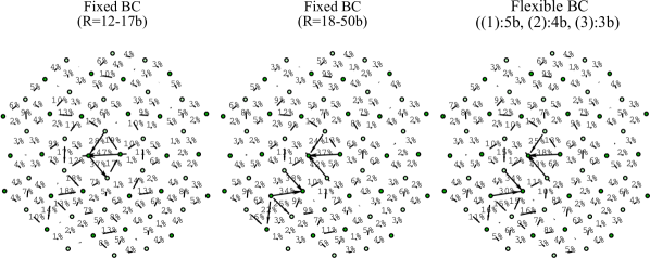
Figure 3: Differential displacement maps of a screw dislocation core in Ti $\left(10\bar{1}2\right)$ twin boundary computed by fixed and flexible boundary conditions. Fixed boundary conditions cause a supercell size effect which is evident from different core structures for radius $R$ smaller or larger than 17b (1312 atoms relaxed). Flexible boundary conditions give the same core structure as the large fixed boundary conditions supercell with significantly less atoms required to relax by energy minimization (i.e 73 atoms in region (1) and 652 atoms total).

The core structure from flexible boundary conditions is in good agreement with large fixed boundary conditions results– hence the correct structure can be obtained using flexible boundary conditions with significantly less atoms than with fixed boundary conditions.

V Conclusions

We developed an automated computational approach to calculate the lattice Green’s function of crystals containing planar interfaces for arbitrary force constants and interface orientations. This method is more general than the previous Dyson-equation approaches in the sense that it can consider long range atomic interactions and reconstructions near the interface. We computed the ILGF for a Ti $\left(10\bar{1}2\right)$ twin boundary with a Ti MEAM potential and studied the screw dislocation/twin boundary interaction using flexible boundary conditions. Our results show that the ILGF flexible boundary conditions method predicts the correct dislocation core structure. Moreover, the energy minimization stage of the flexible boundary conditions involves significantly less atoms than what is required by fixed boundary conditions methods. This highlights the applicability of flexible boundary conditions methods to modeling defect/interface interactions by DFT.

VI Acknowledgments

This work is supported by NSF/CMMI grant 0846624.

Appendix A Evaluation of $\mathbf{\check{\utilde{G}}_{\alpha l,\alpha^{\prime}l^{\prime}}^{\sigma\sigma^{\prime}}(k_{x}=0)}$

A.1 $\sigma=\sigma^{\prime}$

$\check{\utilde{G}}_{\alpha l,\alpha^{\prime}l^{\prime}}^{\sigma\sigma}(k_{x}=0)$ is obtained by taking the limit of Eqn. (III) and Eqn. (13) as $k_{x}\rightarrow 0$:

$$\check{\utilde{G}}_{\alpha l,\alpha^{\prime}l^{\prime}}^{\sigma\sigma}(k_{x}=0) = \int_{k_{i}(0)}^{k_{f}(0)}\utilde{G}^{\sigma\sigma}(k_{z}\hat{z})(e^{-ik_{z}(z_{l}-z_{l^{\prime}})}-1)dk_{z}$$ (27)

$$+ \int_{k_{i}(0)}^{k_{f}(0)}\utilde{G}^{\sigma\sigma}(k_{z}\hat{z})-\frac{\hat{\utilde{G}}^{\sigma\sigma}}{k_{z}^{2}}f_{c}(k_{z})dk_{z}$$ (28)

$$+ \int_{k_{i}(0)}^{k_{f}(0)}\frac{\hat{\utilde{G}}^{\sigma\sigma}}{k_{z}^{2}}(f_{c}(k_{z})-1)dk_{z}$$ (29)

$$+ \displaystyle\lim_{k_{x}\rightarrow 0}\hat{\utilde{G}}^{\sigma\sigma}\left(\frac{\arctan(k_{f}(k_{x})/k_{x})-\arctan(k_{i}(k_{x})/k_{x})}{k_{x}}-\frac{\pi}{|k_{x}|}\right).$$ (30)

Note that since $\vec{k}=k_{z}\hat{z}$, $\hat{\utilde{G}}^{\sigma\sigma}(\hat{k})$ is evaluated along a constant $\hat{k}$-direction and therefore is a constant. The cut off function is

$f_{c}(k_{z})=\Bigg{\{}$ 1 $0<\left|k_{z}\right|<0.5k_{z}^{\text{max}}$ $12(1-\left|k_{z}\right|)^{2}-16(1-\left|k_{z}\right|)^{3}$ $0.5k_{z}^{\text{max}}<\left|k_{z}\right|<k_{z}^{\text{max}}$

where $k_{z}^{\text{max}}\leq\text{Min}(\left|k_{i}(0)\right|,k_{f}(0))$ to insure that $f_{c}(k_{z})=0$ at the Brillouin zone boundary. We isolate the $k_{z}=0$ point by dividing the integration path in Eqn. (27), Eqn. (28) and Eqn. (29) into three intervals

$$\left[k_{i}(0),k_{f}(0)\right]=\left[k_{i}(0),-\epsilon/2\right)\cup\left[-\epsilon/2,\epsilon/2\right]\cup\left(\epsilon/2,k_{f}(0)\right]$$

where $\epsilon$ is sufficiently small. The first and third intervals do not contain the $\Gamma$-point and therefore their corresponding integrals are evaluated numerically without special treatments. To evaluate the integrals in Eqn. (27) and Eqn. (28) over $\left[-\epsilon/2,\epsilon/2\right]$, we use the small $k_{z}$ leading order terms of $\utilde{G}^{\sigma\sigma}(\vec{k})$ ref:lgf and the exponential term

$$\int_{-\epsilon/2}^{\epsilon/2}\utilde{G}^{\sigma\sigma}(k_{z}\hat{z})(e^{-ik_{z}(z_{l}-z_{l^{\prime}})}-1)dk_{z}=\\ \int_{-\epsilon/2}^{\epsilon/2}\left(\frac{\hat{\utilde{G}}_{\alpha\alpha^{\prime}}^{\sigma\sigma}}{k_{z}^{2}}+\frac{i}{\left|k_{z}\right|}{\utilde{G}}_{\alpha\alpha^{\prime}}^{\sigma\sigma,i}\frac{k_{z}}{\left|k_{z}\right|}+\utilde{G}_{\alpha\alpha^{\prime}}^{\text{D}}(k_{z})\right)\left(-ik_{z}(z_{l}-z_{l^{\prime}})-k_{z}^{2}\frac{(z_{l}-z_{l^{\prime}})^{2}}{2}\right)dk_{z}=\\ \left({\utilde{G}}_{\alpha\alpha^{\prime}}^{\sigma\sigma,i}(z_{l}-z_{l^{\prime}})-\hat{\utilde{G}}_{\alpha\alpha^{\prime}}^{\sigma\sigma}\frac{(z_{l}-z_{l^{\prime}})^{2}}{2}\right)\epsilon$$

and

$$\int_{-\epsilon/2}^{\epsilon/2}\utilde{G}^{\sigma\sigma}(k_{z}\hat{z})-\frac{\hat{\utilde{G}}^{\sigma\sigma}}{k_{z}^{2}}f_{c}(k_{z})dk_{z}=\int_{-\epsilon/2}^{\epsilon/2}\left(i\frac{{\utilde{G}}_{\alpha\alpha^{\prime}}^{\sigma\sigma,i}}{k_{z}}+\utilde{G}_{\alpha\alpha^{\prime}}^{\text{D}}(k_{z})\right)dk_{z}=\utilde{G}_{\alpha\alpha^{\prime}}^{\text{D}}(0)\epsilon.$$

$\hat{\utilde{G}}_{\alpha\alpha^{\prime}}^{\sigma\sigma}/k_{z}^{2}$ and $\utilde{G}_{\alpha\alpha^{\prime}}^{\text{D}}(k_{z})$ are the elastic and discontinuity corrections and $i{\utilde{G}}_{\alpha\alpha^{\prime}}^{\sigma\sigma,i}/k_{z}$ appears only in the case of a multiatom basis. $\hat{\utilde{G}}_{\alpha\alpha^{\prime}}^{\sigma\sigma}$ and $\utilde{G}_{\alpha\alpha^{\prime}}^{\sigma\sigma,i}$ are constants hereref:lgf ; ref:effic . Also note that $f_{c}(k_{z})=1$ over $\left[-\epsilon/2,\epsilon/2\right]$; hence the integral in Eqn. (29) equals zero over this interval.

Taking $\epsilon$ to be $\frac{k_{f}(0)-k_{i}(0)}{N_{\text{div}}}$ where $N_{\text{div}}$ is the number of divisions in the discrete $k_{z}$ mesh we have

$$\check{\utilde{G}}_{\alpha l,\alpha^{\prime}l^{\prime}}^{\sigma\sigma}(0) = \frac{k_{f}(0)-k_{i}(0)}{N_{\text{div}}}\Bigg{[}\sum_{k_{z}\neq 0}\left(\utilde{G}_{\alpha\alpha^{\prime}}^{\sigma\sigma}(k_{z}\hat{z})e^{-ik_{z}(z_{l}-z_{l^{\prime}})}-\frac{\hat{\utilde{G}}^{\sigma\sigma}}{k_{z}^{2}}\right)$$

$$+ \utilde{G}_{\alpha\alpha^{\prime}}^{\sigma\sigma,i}(z_{l}-z_{l^{\prime}})-\frac{\hat{\utilde{G}}_{\alpha\alpha^{\prime}}^{\sigma\sigma}(z_{l}-z_{l^{\prime}})^{2}}{2}+\utilde{G}_{\alpha\alpha^{\prime}}^{\text{D}}(0)\Bigg{]}$$

$$+ \hat{\utilde{G}}_{\alpha\alpha^{\prime}}^{\sigma\sigma}\left(\frac{1}{k_{i}(0)}-\frac{1}{k_{f}(0)}\right).$$

The first summation

$\displaystyle\frac{k_{f}(0)-k_{i}(0)}{N_{\text{div}}}\sum_{k_{z}\neq 0}\left(\utilde{G}_{\alpha\alpha^{\prime}}^{\sigma\sigma}(k_{z}\hat{z})e^{-ik_{z}(z_{l}-z_{l^{\prime}})}-\frac{\hat{\utilde{G}}^{\sigma\sigma}}{k_{z}^{2}}\right)=$

$\displaystyle\frac{k_{f}(0)-k_{i}(0)}{N_{\text{div}}}\sum_{k_{z}\neq 0}{\left(\utilde{G}_{\alpha\alpha^{\prime}}^{\sigma\sigma}(k_{z}\hat{z})(e^{-ik_{z}(z_{l}-z_{l^{\prime}})}-1)\right)+\left(\utilde{G}^{\sigma\sigma}(k_{z}\hat{z})-\frac{\hat{\utilde{G}}^{\sigma\sigma}}{k_{z}^{2}}f_{c}(k_{z})\right)+\left(\frac{\hat{\utilde{G}}^{\sigma\sigma}}{k_{z}^{2}}(f_{c}(k_{z})-1)\right)}$

is the numerical integration of all three integrals in Eqn. (27)-(29) over $\left[k_{i}(0),-\epsilon/2\right)\cup\left(\epsilon/2,k_{f}(0)\right]$. The last term $\hat{\utilde{G}}_{\alpha\alpha^{\prime}}^{\sigma\sigma}\left(\frac{1}{k_{i}(0)}-\frac{1}{k_{f}(0)}\right)$ is the evaluation of Eqn. (30).

A.2 $\sigma\neq\sigma^{\prime}$

$\check{\utilde{G}}_{\alpha\alpha^{\prime}}^{\sigma\sigma^{\prime}}(k_{x}=0)$ is obtained from the small $k_{x}$ expansion of Eqn. (9) and removing the $k_{x}^{-1}$ term

$$\check{\utilde{G}}_{\alpha\alpha^{\prime}}^{\sigma\sigma^{\prime}}(0)=\frac{\pi}{\left|\vec{t}_{2}\right|}\left(2a_{\alpha\alpha^{\prime}}^{qq^{\prime}}\left|\beta_{l,l^{\prime}}^{qq^{\prime}}\right|-b_{\alpha\alpha^{\prime}}^{qq^{\prime}}\gamma_{l,l^{\prime}}^{qq^{\prime}}\right).$$ (31)

References

(1)
J. E. Sinclair, P. C. Gehlen, R. G. Hoagland, and J. P. Hirth,
J. Appl. Phys. 49, 3890 (1978).
(2)
R. Thomson, S. J. Zhou, A. E. Carlsson, and V. K. Tewary,
Phys. Rev. B 46, 10613 (1992).
(3)
L. M. Canel, A. E. Carlsson, and R. Thomson,
Phys. Rev. B 52, 158 (1995).
(4)
S. Rao, C. Hernandez, J. P. Simmons, T. A. Parthasarathy, and C. Woodward,
Phil. Mag. A 77, 231 (1998).
(5)
S. I. Rao and C. Woodward,
Phil. Mag. A 81, 1317 (2001).
(6)
L. H. Yang, P. Soderlind, and J. Moriarty,
Phil. Mag. A 81, 1355 (2001).
(7)
S. Rao, T. A. Parthasarathy, and C. Woodward,
Phil. Mag. A 79, 1167 (1999).
(8)
C. Woodward and S. I. Rao,
Phil. Mag. A 81, 1305 (2001).
(9)
C. Woodward and S. I. Rao,
Phil. Mag. 84, 401 (2004).
(10)
C. Woodward, D. R. Trinkle, L. G. Hector, and D. L. Olmsted,
Phys. Rev. Lett. 100, 045507 (2008).
(11)
C. Woodward and S. I. Rao,
Phys. Rev. Lett. 88, 216402 (2002).
(12)
V. K. Tewary and R. Thomson,
J. Mater. Res. 7, 1018 (1992).
(13)
A. A. Maradudin, E. Montroll, G. Weiss, and I. Ipatova,
Theory of lattice dynamics in the harmonic approximation,
Solid State Physics, Supp. 3, Academic Press, 1971.
(14)
D. R. Trinkle,
Phys. Rev. B 78, 014110 (2008).
(15)
M. Ghazisaeidi and D. R. Trinkle,
Phys. Rev. E 79, 037701 (2009).
(16)
V. K. Tewary, R. H. Wagoner, and J. P. Hirth,
J. Mater. Res. 4, 113 (1989).