Magnetic structure and magnetoelectric coupling in bulk and thin film FeVO₄

Abstract

We have investigated the magnetoelectric and magnetodielectric response in FeVO₄, which exhibits a change in magnetic structure coincident with ferroelectric ordering at $T_{N2}$$\approx$15 K. Using symmetry considerations, we construct a model for the possible magnetoelectric coupling in this system, and present a discussion of the allowed spin structures in FeVO₄. Based on this model, in which the spontaneous polarization is caused by a trilinear spin-phonon interaction, we experimentally explore the magnetoelectric coupling in FeVO₄  thin films through measurements of the electric field induced shift of the multiferroic phase transition temperature, which exhibits an increase of 0.25 K in an applied field of 4 MV/m. The strong spin-charge coupling in FeVO₄  is also reflected in the significant magnetodielectric shift, which is present in the paramagnetic phase due to a quartic spin-phonon interaction and shows a marked enhancement with the onset of magnetic order which we attribute to the trilinear spin-phonon interaction. We observe a clear magnetic field induced dielectric anomaly at lower temperatures, distinct from the sharp peak associated with the multiferroic transition, which we tentatively assign to a spin reorientation cross-over. We also present a magnetoelectric phase diagram for FeVO₄.

I INTRODUCTION

Magnetoelectric multiferroics, insulating magnets exhibiting simultaneous magnetic and ferroelectric order, are widely investigated in large part due to their potential applications for developing novel devices, including magnetic sensors and multistate memory, among others [ABHGL, ; saf2006, ]. The cross-control of these distinct order parameters, such as adjusting the magnetization using an applied electric field or vice-versa, is expected to provide an extra degree of freedom in developing new types of spin-charge coupled devices, such as voltage switchable magnetic memories [Eeren2007, ]. Additionally, there are a number of fundamental materials questions surrounding the development of multiferroic order. Magnetic and ferroelectric order are generally contraindicated in the same phase, as ferromagnetism in transition metal systems typically requires partially filled d-orbitals while ferroelectric distortions are promoted in a d⁰ electronic configuration[Hill2000, ]. Despite this apparent restriction, a rather large number of single phase systems have been identified as magnetoelectric multiferroics [TK2005, ; Hur2004, ; Lawes2005, ]. A number of microscopic mechanisms have been proposed for the development of multiferroic order, including, a magnetic Jahn-Teller distortion[JT, ] for TbMn₂O₅,[LCC2004, ] bond and site ordering having distinct centers of inversion symmetry,[Efremov2004, ] a microscopic mechanism leading to a spin-current interaction[Katsura2005, ], the Dzyloshinskii-Moriya interaction,[SergienkoPRB, ] a general anisotropic exchange striction,[HYAE, ] a spin-phonon interaction,[Tackett, ] and a strain induced ferroelectricity.[RABE3, ]

Phenomenologically, magnetically-induced ferroelectric order developing in systems having multiple magnetic phases can be understood by considering a trilinear term in the magnetoelectric free energy, F_ME, coupling the electric polarization with two distinct order parameters $\sigma_{1}$ and $\sigma_{2}$ which together break inversion symmetry so that F${}_{ME}\propto$P$\sigma_{1}\sigma_{2}$[ABHGL, ; Lawes2005, ; MKPRL, ; ABHJAP, ; ABHPRB, ]. Since the free energy must transform as a scalar, there are strong symmetry restrictions on the allowed representations for $\sigma_{1}$ and $\sigma_{2}$; in particular, the product $\sigma_{1}({\bf q})\sigma_{2}({\bf q})^{*}$ must be antisymmetric under spatial inversion. This trilinear coupling also predicts electric field control of a magnetic order parameter[ABHGL, ; Kharel2009, ]. A general discussion of the symmetry of the magnetoelectric coupling in multiferroics is considered for the specific case of FeVO₄  in the following section. Investigations on multiferroic Ni₃V₂O₈  thin films, in which such a trilinear coupling is believed to be responsible for the multiferroic order[ABHGL, ; Lawes2005, ], have established that the multiferroic transition temperature can be varied through the application of either (or both) magnetic and electric fields [Kharel2009, ], confirming the strong coupling between magnetic and dielectric degrees of freedom. Higher order magnetoelectric coupling terms quadratic in both magnetic and ferroelectric terms will give rise to magnetization induced shift in the dielectric response[RABE1, ]. Such coupling has been investigated both theoretically and experimentally in a range of materials including Mn₃O₄[Tackett, ], CoCr₂O₄[LawesMelot, ], BaMnF₄[Samara1976, ; Fox1977, ; Fox1979, ; Scott1977, ], and SeCuO₃ and TeCuO₃[Lawes2003, ]. Because this magnetodielectric coupling is also expected to depend strongly on the symmetry of the magnetic phase, it has been suggested that changes in this coupling may be used to probe changes in the ordered spin structure[Tackett, ].

Triclinic iron vanadate, FeVO₄, has recently been identified as a multiferroic system having the P$\overline{1}$ space group [Dixit2009, ; Daoud2009, ; Kundys2009, ]. Magnetic, thermodynamic, and neutron diffraction studies on FeVO₄  single crystal and ceramic samples have shown that FeVO₄  transitions from a paramagnetic phase into a collinear incommensurate (CI) phase at $T_{N1}$=22 K and then into non-collinear incommensurate (NCI) phase at $T_{N2}$=15 K.[Dixit2009, ; Daoud2009, ; Kundys2009, ; He2008, ] Ferroelectric order in FeVO₄ develops in this non-collinear spiral magnetic phase. The onset of ferroelectric order with the development of a second magnetic phase suggests that a symmetry-based approach may be useful in exploring the multiferroic properties in this system. We present a full Landau theory for this system, specifically considering the allowed magnetoelectric coupling terms. Our result is that a nonzero induced spontaneous polarization ${\vec{P}}$ requires having a magnetic spiral[MOST, ] described by two order parameters which are out of phase with respect to one another.[Lawes2005, ; MKPRL, ; ABHGL, ; ABHPRB, ] In this low symmetry structure there are no restriction on the orientation of ${\vec{P}}$ based on symmetry arguments, unlike the majority of similar magnetically-induced multiferroics[ABHGL, ; Lawes2005, ; MKPRL, ; MOST, ].

This paper is organized as follows. In Sec. II we present a symmetry analysis of FeVO₄ based on Landau theory. Here we analyze the symmetry of the magnetoelectric interaction. In Sec. III we present the results of a number of experiments designed to probe the structure of these magnetoelectric interactions. In Sec. IV we briefly summarize our results.

II Landau Theory

Motivated by this general discussion of the possibility of magnetically driven ferroelectric order in FeVO₄, we now present a Landau theory for FeVO₄  with some details of the construction relegated to the the Appendix. As discussed in detail in Ref. [ABHPRB, ], the Fourier transform of the spin ordering is proportional to the critical eigenvector of the inverse susceptibility matrix at the ordering wave vector $\vec{q}$. In the Appendix we analyze the constraint of spatial inversion in the P$\overline{1}$ space group of the paramagnetic phase, with the following results. The FeVO₄  structure consists of six $S$=5/2 Fe³⁺ spins in the unit cell at locations ${\mbox{\boldmath{$\tau$}}}_{n}$. For $n=1,2,3$, $-{\mbox{\boldmath{$\tau$}}}_{n}=\overline{\mbox{\boldmath{$\tau$}}}_{n}=\tau_{n+3}$ and $-{\mbox{\boldmath{$\tau$}}}_{n+3}=\overline{\mbox{\boldmath{$\tau$}}}_{n+3}={\mbox{\boldmath{$\tau$}}}_{n}$. Then inversion symmetry (${\cal I}$) implies that spin Fourier transform obeys

$${\cal I}\vec{S}(\vec{q},\tau)=\vec{S}(\vec{q},\overline{\tau})^{*}\,$$ (1)

where, as defined in the Appendix, $\vec{S}(\vec{q},\tau)$ is the spatial Fourier transform of the thermally averaged spin operator. As explained in the Appendix, this relation implies that the spin distribution is inversion-symmetric about some origin. We find that inversion symmetry implies that

$$[S_{x}(1),S_{y}(1),S_{z}(1),S_{x}(2),S_{y}(2)\dots S_{z}(6)] = \sigma_{n}[x_{1}^{*},y_{1}^{*},z_{1}^{*},x_{2}^{*},y_{2}^{*},...z_{6}^{*}]\$$ (2)

where all the components are complex valued with $x_{\overline{n}}=x_{n}^{*}$, $y_{\overline{n}}=y_{n}^{*}$, $z_{\overline{n}}=z_{n}^{*}$, are normalized by $\sum_{n=1}^{6}[|x_{n}|^{2}+|y_{n}|^{2}+|z_{n}|^{2}]=1$, and the wave vector argument is implicit. The amplitude $\sigma_{n}(\vec{q})$ is the complex valued magnetic order parameter, which obeys

$${\cal I}\sigma_{n}(\vec{q})=\sigma_{n}(\vec{q})^{*}=\sigma_{n}(-\vec{q})\ .$$ (3)

As noted in the Appendix, this relation implies that each $\sigma_{n}$ is inversion invariant about a lattice point (which depends on $n$) where the order parameter wave has its origin. As the temperature is lowered one passes from the paramagnetic phase into a phase with an order parameter $\sigma_{1}(\vec{q})$ and then, at a lower temperature into a phase where two order parameters $\sigma_{1}(\vec{q})$ and $\sigma_{2}(\vec{q})$ are nonzero, both of which obey Eq. (3), but which have different centers of inversion symmetry.

The total magnetoelectric free energy, $F_{\rm ME}$ can be written as

$$F_{\rm ME} = F_{\rm M}+F_{\rm E}+V\ ,$$ (4)

where $F_{\rm M}$ is the purely magnetic free energy, $F_{\rm E}$ is the dielectric potential which we approximate as $F_{\rm E}=(1/2)\chi_{E}^{-1}{\bf P}^{2}$, where $\chi_{E}$ is the dielectric susceptibility (whose crystalline anisotropy is neglected), and to leading order in $\sigma_{n}$, the magnetoelectric coupling term is given by:

$$V = \sum_{n,m=1}^{2}\sum_{\gamma}[a_{n,m,\gamma}\sigma_{n}(\vec{q})\sigma_{m}(\vec{q})^{*}+a_{n,m,\gamma}^{*}\sigma_{n}(\vec{q})^{*}\sigma_{m}(\vec{q})]P_{\gamma}\ ,$$ (5)

where $n$ and $m$ label order parameter modes and $\gamma$ labels the Cartesian component of $\vec{P}$. Terms linear in $\sigma_{n}$ are prohibited because they are not time reversal invariant and also can not conserve wave vector. The magnetoelectric interaction $V$ has to be inversion invariant and the appendix shows that the $a$ coefficients are pure imaginary, so that

$$V = i\sum_{\gamma}r_{\gamma}[\sigma_{1}(\vec{q})\sigma_{2}(\vec{q})^{*}-\sigma_{1}(\vec{q})^{*}\sigma_{2}(\vec{q})]P_{\gamma}=2\sum_{\gamma}r_{\gamma}|\sigma_{1}(\vec{q})\sigma_{2}(\vec{q})|\sin(\phi_{2}-\phi_{1})P_{\gamma}\ ,$$ (6)

where $\sigma_{n}(\vec{q})=|\sigma_{n}(\vec{q})|\exp(i\phi_{n})$. There is no restriction on the direction of the spontaneous polarization, so that all components of $\vec{P}$ will be nonzero. However, if the magnetic structure is a spiral, then the arguments of Mostovoy[MOST, ] might be used to predict the approximate direction of $\vec{P}$. The result of Eq. (6) is quite analogous to that for Ni₃V₂O₈[Lawes2005, ] or for TbMnO₃[MKPRL, ], in that it requires the presence of two modes $\sigma_{1}(\vec{q})\equiv\exp(i\phi_{1})|\sigma_{1}(\vec{q})|$ and $\sigma_{2}(\vec{q})\equiv\exp(i\phi_{2})|\sigma_{2}(\vec{q})|$ which are out of phase with one another: $\phi_{1}\not=\phi_{2}$. Then the order parameter wavefunctions have different origins and will therefore break inversion symmetry.

If, as stated in Ref. Daoud2009, , the eigenvector is not inversion invariant as implied by Eq. (3), then one would conclude that the magnetic ordering transition is not continuous. However, the most likely scenario is that the ordering transitions are continuous and that the spin distribution for each $\sigma_{n}(\vec{q})$ is inversion symmetric as obtained in this derivation. The acentric distribution found in Ref. Daoud2009, differs only slightly from being inversion symmetric for reasons that are obscure.[PGRPC, ]

III Magnetoelectric Interactions (Experimental)

III.1 Sample Synthesis and Structural Characterization

Motivated by Eq. (6), which predicts that the magnetic structure defined by $\sigma_{1}(\vec{q})$ and $\sigma_{2}(\vec{q})$ is coupled to the electric polarization $P$, we experimentally investigated the nature of the higher order magnetoelectric coupling in FeVO₄. Bulk single phase polycrystalline iron vanadate (FeVO₄) ceramic samples were prepared using standard solid state reactions. Because Eq. 6 predicts that all components of the polarization vector are nonzero, and previous measurements on ceramic FeVO₄  have found clear evidence for multiferroic behaviour [Dixit2009, ] we focused our study on polycrytalline samples. A stoichiometric ratio of iron oxide (Fe₂O₃) and vanadium pentaoxide (V₂O₅) solid solutions were thoroughly mixed and ground to produce a homogeneous mixture. This mixture was slowly heated to 600^oC for 4 hours in air. Intermediate grindings followed by thermal annealing in air were repeated several times to complete the solid state reaction and ensure a fully reacted and uniform composition. This homogeneous solid solution was finally annealed in air at 800^oC for 4 hours, yielding a yellowish brown powder identified as a single phase iron vanadate by X-ray diffraction and Raman spectroscopy.

In order to apply large electric fields to FeVO₄  we also prepared thin film samples. These were fabricated from a phase pure stoichiometric iron vanadate target. The FeVO₄ powder used for the sputtering target was prepared by the method described above. Approximately 30 g of FeVO₄ powder was mixed with 15 mL of 2 mole percent polyvinyl alcohol as a binder. The dried powder was pressed into a circular disc having a diameter of approximately 50 mm with a thickness of roughly 3.5 mm followed by air annealing at 600^oC for 4 hours to burn off the residual organics. A final thermal annealing was done at 800^oC for 4 hours to produce the dense pellet used for the sputtering target. FeVO₄ films were deposited at room temperature using RF magnetron sputtering onto conducting silicon substrates. The working pressure was held at 1.5x10^-2 torr, with the atmosphere consisting of a mixture of approximately 1.5x10^-3 torr partial pressure of oxygen as the reactive gas and approximately 1.35x10^-2 torr partial pressure of argon as the sputtering gas. These as deposited films, prepared over a time of 4 hours, were amorphous. After air annealing at 700^oC for 4 hours the films were indexed as single phase polycrystalline FeVO₄.

We investigated the structural, magnetic, and electronic properties of these samples using a number of different techniques. We used a Rigaku RU200 powder X-ray diffractometer and Horiba Triax Raman spectrometer to study the crystalline structure of these samples. We used a Hitachi scanning electron microscope (SEM) to investigate the surface morphology of the thin film samples and an associated energy dispersive X-ray (EDX) assembly to probe the chemical composition of both samples. We measured the temperature dependent magnetization of the powder sample using a Quantum Design MPMS SQUID magnetometer, although the very small magnetic anomalies associated with the transitions could not be clearly distinguished from background in the thin films samples. We conducted temperature and field dependent dielectric and pyrocurrent measurements using the temperature and field control provided by a Quantum Design PPMS system used in conjunction with an Agilent 4284A LCR meter and a Keithley 6517 electrometer. These measurements were done on a cold pressed pellet of bulk FeVO₄ with the top and bottom electrodes fashioned using silver epoxy and on the FeVO₄ thin films with room sputtered gold (Au) used as the top electrode and the Si substrate serving as the bottom electrode.

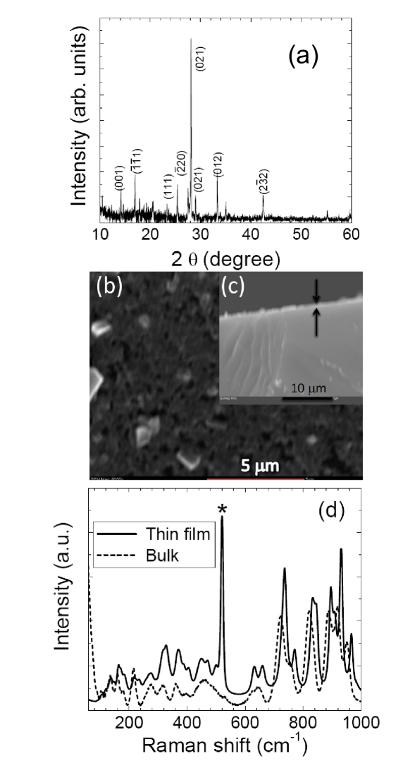
Figure 1: (a) $\theta$-2$\theta$ x-ray diffraction (XRD) pattern of FeVO₄  thin film, (b) Surface scanning electron micrograph of FeVO₄  thin film, (c) Cross-sectional SEM image of FeVO₄, thin film and (d) room temperature Raman spectrum on FeVO₄  bulk powder and thin film samples. The peak at 560 cm^-1 (indicated by an asterisk) arises from the silicon substrate

The structure of the ceramic FeVO₄ sample was practically identical to that previously presented for a bulk sample prepared using a different technique [Dixit2009, ]. The X-ray diffraction (XRD) pattern for the FeVO₄ thin film is shown in Fig 1(a). These diffraction peaks are consistent with the expected XRD pattern for FeVO₄ [JCPDS no. 38-1372]. The surface morphology the thin film sample is shown in Fig 1(b). This SEM micrograph indicates that the film consists of grains with various orientations, as well as a number of pinhole defects. We calculated the thickness of these thin films to be roughly 200 nm, using the cross-sectional SEM micrograph, Fig 1(c). This value is very consistent with estimates from well defined interference fringes observed in reflection spectra (not shown). EDX analysis of both the bulk and thin film samples show a 1:1 iron to vanadium ratio. We carried out room temperature Raman vibrational spectroscopy to further probe the microstructures of both bulk and thin films. The identification of Raman active modes and their detailed temperature dependent analysis on bulk FeVO₄ sample is discussed elsewhere [Dixit2009, ]. Here we plot the room temperature Raman spectrum of both bulk and thin film FeVO₄ in Fig1(d). We are able to identify all the Raman active modes for thin films, which are observed in bulk FeVO₄ [Dixit2009, ] with a small shift in the Raman peaks for the thin films. The Raman peak arising from the silicon substrate is indicated by an asterisk.

III.2 Temperature Dependent Dielectric Measurements on FeVO₄  Ceramic

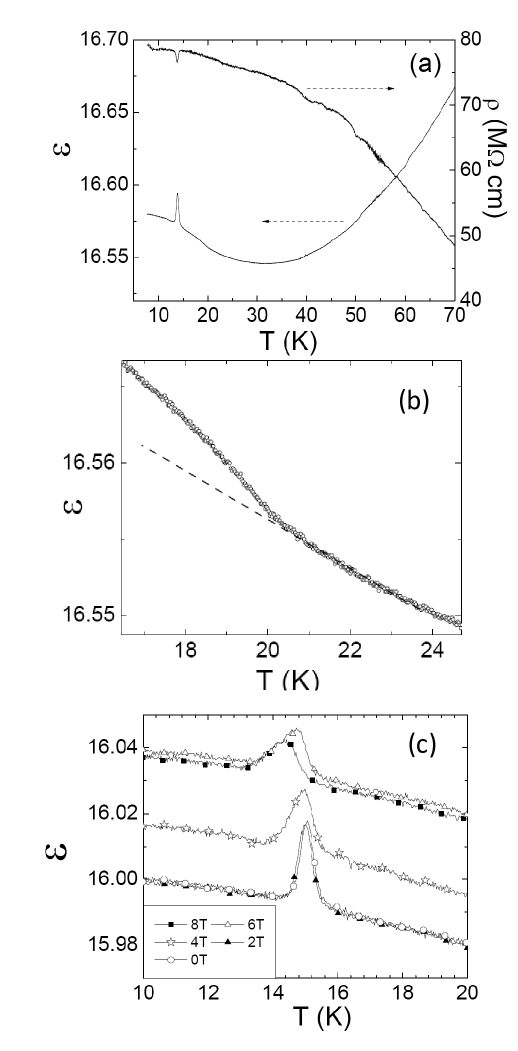
Figure 2: (a) Zero field temperature dependent dielectric constant (left axis) and resistivity (right axis) for ceramic FeVO₄  sample, (b) Temperature dependence of the dielectric constant near the magnetic ordering temperature, and (c) Temperature dependence of dielectric constant at $H$= 0, 20, 40, 60, and 80 kOe. The dashed line in (b) is a guide to the eye.

The temperature dependent magnetization for the bulk FeVO₄ sample (not shown) was practically identical to that measured previously on a different ceramic sample prepared using a different technique [Dixit2009, ]. In particular, the magnetization showed the usual two anomalies associated with the two incommensurate transitions in this system. We plot the zero-field dielectric constant and resistivity for bulk FeVO₄ over a broad range of temperatures in Fig. 2(a). The dielectric constant exhibits a sharp peak near $T_{N2}$, arising from the development of ferroelectric order in the incommensurate spiral magnetic phase. As shown in Fig. 2(a), above 35 K, the dielectric constant for FeVO₄ shows a gradual decrease on cooling, typical of many insulating materials [Ramirez2000, ]. Below roughly 30 K, the dielectric constant increases smoothly with further cooling. Since the resistivity of FeVO₄ increases monotonically with decreasing temperature (except for a small anomaly at $T_{N2}$), also shown in Fig. 2(a), we attribute this increase in the dielectric constant to a quartic magnetoelectric coupling, $V_{4}$. Although FeVO₄ does not order magnetically until cooled below $T_{N1}$=22 K, heat capacity measurements suggest the presence of short range spin correlations developing well above this temperature [Dixit2009, ]. It has been suggested in a number of other systems, including TeCuO₃ [Lawes2003, ] and Mn₃O₄ [Tackett, ], that short-range magnetic correlations can produce magnetodielectric corrections; we propose that the same mechanism is responsible for the non-monotonic temperature dependence of the dielectric constant of FeVO₄ in the paramagnetic phase.

The fourth order magnetoelectric coupling contains terms quadratic in $\vec{P}$ and $\sigma_{n}(\vec{q})$. If $\sigma_{1}(\vec{q})$ is the order parameter that develops at $T_{N1}$, then this coupling is probably dominated by $\lambda|\vec{P}|^{2}|\sigma_{1}(\vec{q})|^{2}$ at high temperatures. The finite spin correlations developing above $T_{N1}$ cause $\langle|\sigma_{1}(\vec{q})|^{2}\rangle$ to be nonzero so that the coupling term is in effect $a|\vec{P}|^{2}$, where $a=\lambda\langle|\sigma_{1}(\vec{q})|^{2}\rangle$. This term produces a shift in the dielectric constant in the paramagnetic phase, as seen in Fig. 2(a) below approximately 30 K. Below $T_{N1}$, approximately 22 K, when $\sigma_{1}(\vec{q})$ acquires a finite expectation value, a trilinear coupling term $a\vec{P}<\sigma_{1}(\vec{q})>\sigma_{2}(\vec{q})^{*}$ is allowed. This term will lead to mode mixing so that the critical mode approaching $T_{N2}$ is not $\sigma_{2}(\vec{q})$ but $(\sigma_{2}(\vec{q})+\rho\vec{P})$ where $\rho$ is of order $a\langle\sigma_{1}(\vec{q})\rangle$ [ABHPRB, ]. Then the divergence in this variable as $T_{N2}$ is approached will lead to a simultaneous divergence (with a very much reduced amplitude) in the observed dielectric constant. This mode mixing is therefore expected to lead to a slight increase in the magnetodielectric shift below $T_{N1}$ [ABHPRB, ]. This is seen clearly in Fig. 2b, where the dashed line shows the extrapolation of the magnetodielectric shift from $T>T_{N1}$ to $T<T_{N1}$, an extrapolation that does not include any corrections arising from the trilinear magnetoelectric term.

III.3 Magnetic Field Dependent Dielectric Measurements on FeVO₄  Ceramic

To further investigate spin-charge coupling in FeVO₄, we plot the temperature dependent dielectric constant measured at different magnetic fields in Fig 2(c). We find that the dielectric anomaly signaling the onset of ferroelectric order shifts to lower temperatures with increasing magnetic field, with the reduction in transition temperature reaching 0.7 K in a magnetic field of $H$=80 kOe. This result is expected, as the ferroelectric order producing the dielectric anomaly is associated with the incommensurate spiral transition, which typically show a reduction in transition temperature in applied magnetic fields.

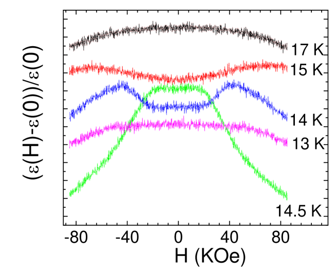
Figure 3: (color on-line)Magnetic field dependence of the relative change in the dielectric constant for ceramic FeVO₄  at different temperatures with vertical offset included for clarity.

We conducted additional measurements of the dielectric response of the bulk sample while sweeping the magnetic field at fixed temperature. These results are shown in Fig. 3, plotted as $\Delta\epsilon(H)/\epsilon(H=0)$ versus $H$ with data measured at different temperatures offset vertically for clarity. At $T$=17 K, which is intermediate between $T_{N1}$ and $T_{N2}$, there is a small negative magnetocapacitance, with the dielectric constant being reduced by approximately 0.03% in a field of $H$=80 kOe. As the temperature approaches the multiferroic transition at $T_{N2}$, the magnetodielectric coupling shows qualitative changes. By $T$=15 K the magnetocapacitive shift is positive for small fields, with a shift in dielectric constant on the order of 0.02% at high magnetic fields. The magnetocapacitive response is maximal near $T$=14.5 K, with the dielectric constant being reduced by approximately 0.1% in a field of $H$=80 kOe. At still lower temperatures the magnitude of the magnetocapacitive shift becomes smaller.

Perhaps the most dramatic feature in the isothermal magnetocapacitance curves presented in Fig. 3 is the presence of clear maxima, which vary as a function of temperature and magnetic field. These maxima appear first at small fields at $T$=14.5 K, then shift to larger fields as the temperature is reduced. We believe that these anomalies do not reflect the suppression of the multiferroic transition temperature in a magnetic field, as discussed in the context of Fig 2(b). These isothermal dielectric anomalies persist to temperatures 2 K or 3 K below $T_{N2}$, while the maximum suppression of $T_{N2}$ was only 0.7 K over the field range studied, as determined from the measurements in Fig. 3. We propose that this dielectric anomaly may indicate a spin-reorientation transition in FeVO₄. The magnetodielectric coupling is expected to depend on the symmetry of the magnetically ordered state [Lawes2003, ; ABHPRB, ], so a field induced spin reorientation crossover could potentially produce the low temperature dielectric anomalies observed in Fig. 3. Similar magnetic field-induced dielectric anomalies have been observed in other materials including Mn₃O₄ [Tackett, ], although the specific mechanisms responsible remain unclear. One possibility is that the external magnetic field serves to reduce the slight geometrical frustration present in FeVO₄ [Daoud2009, ], allowing a different spin structure to emerge. Alternatively, the spin orientation could be a spin-flop transition as seen in TbMnO₃.[Aliouane2006, ] We note, however, that FeVO₄ remains ferroelectric at high magnetic fields [Dixit2009, ], so the modified spin structures would still need to transform as defined by Eq. 3.

III.4 Magnetoelectric Coupling in FeVO₄  Thin Films

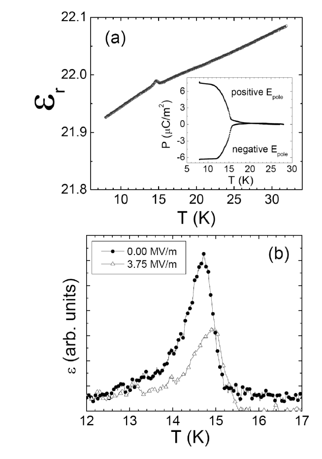
Figure 4: (a) Temperature dependence of dielectric constant for FeVO₄  thin films at zero field, Inset: Zero magnetic field polarization for FeVO₄  thin film measured at poling fields E_pole = $\pm$10 MV m^-1 and (b) Temperature dependent dielectric constant measured at E=0 and E=3.75 MV m^-1 (background was subtracted for clarity)

The trilinear magnetoelectric coupling that produces multiferroic order, given in Eq. 6, also results in an electric field ($\vec{E}$) dependence of the magnetic structure through the coupling term in the free energy $\Delta F=-\vec{P}\cdot\vec{E}$. We first confirmed that these thin film samples were also multiferroic, through measurements of the dielectric constant and pyrocurrent, illustrated in Fig. 4(a). The dielectric constant for the thin film FeVO₄ is slightly higher than that found for the ceramic sample. We attribute this discrepancy mainly to the uncertainty in accurately determining the geometrical factor for these thin films. The dielectric response for these thin film samples is approximately independent of measuring frequency and the loss for these films is tan $\delta\approx$ 0.01, which may be due to the presence of pinhole defects in the thin film sample as seen in the SEM micrograph in Fig. 1(b). The zero-field temperature dependent dielectric constant, measured at $f$=30 kHz, is plotted in Fig. 4(a). There is a sharp peak near $T_{N2}$=15 K, associated with the development of ferroelectric order in these thin film samples. We note that, unlike the measurements on bulk FeVO₄ shown in Fig. 2(a), the background dielectric constant for FeVO₄ decreases monotonically with decreasing temperature. This behaviour can be associated with the much larger conductivity of the thin film sample, arising from the presence of the pinhole defects, which obscures the low temperature increase in dielectric constant observed in bulk FeVO₄ (Fig. 2(a)).

We confirmed that the low temperature phase of the FeVO₄ thin film is ferroelectric by integrating the pyrocurrent after poling at positive and negative fields to yield the spontaneous polarization. These results are shown in the inset to Fig. 4(a) and indicate a spontaneous polarization of 6 $\mu$C/m², consistent with previous measurements on polycrystalline bulk FeVO₄ [Dixit2009, ] Measurements of the dielectric response for FeVO₄ thin films under applied magnetic fields (not shown) yield a suppression of the multiferroic transition temperature very similar to that observed in bulk FeVO₄ (see Fig. 2(b)).

To probe the electric field control of the multiferroic phase transition temperature, expected from the nature of the magnetoelectric coupling, we measured the temperature dependent dielectric response in the FeVO₄ thin film sample as a function of bias voltage. Focusing on thin film samples allows the application of relatively large electric fields (on the order of MV/m) with small applied bias voltages. We chose to probe the transition through dielectric measurements as the magnetic anomaly at $T_{N2}$ cannot be clearly discerned in these thin film samples. We plot the temperature dependent dielectric constant measured at E=0 and E=3.75 MV/m in Fig. 4(b). With the application of an electric field, the dielectric peak shifts upwards in temperature, by approximately 0.25 K in a field of E=3.75 MV/m. We note that any sample heating, which is expected to be negligible in any case because of the low dissipation, would raise the sample temperature relative to the thermometer temperature, leading to an apparent decrease in transition temperature, rather than the increase seen in Fig. 4(b). This increase in transition temperature is consistent with an external electric field promoting the development of ferroelectric order, and is similar to what has been observed previously in multiferroic Ni₃V₂O₈  films [Kharel2009, ]. The relatively small increase of the ferroelectric transition under such large applied electric fields can be directly attributed to the very small polarization in FeVO₄. We confirmed that the dielectric anomaly in Fig. 4(b) can still be associated with the multiferroic transition, even in the presence of an electric field, by measuring the response under the simultaneous application of magnetic and electric fields (not shown). Although the dielectric peak broadens considerably, the continuing presence of a single peak under such crossed fields is strong evidence that this anomaly reflects the multiferroic transition in FeVO₄.

III.5 Magnetoelectric phase diagram for FeVO₄

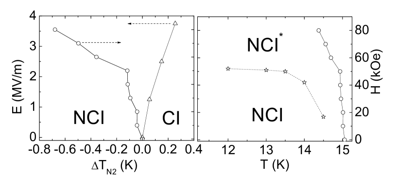
Figure 5: (a) Electric and magnetic field dependence of the multiferroic transition temperature $T_{N2}$ and (b) Magnetic field dependence of multiferroic transition temperature together with the proposed magnetic field induced spin reorientation cross over. Here, NCI^∗ indicates the proposed phase having a spin reoriented structure

We summarize the results of these magnetoelectric and magnetodielectric studies on FeVO₄ in Figs 5(a) and 5(b). We plot the E-field and H-field dependence of the multiferroic transition temperature in FeVO₄ ($T_{N2}$) in Fig. 5(a), where CI and NCI represent the incommensurate magnetic structures below $T_{N1}$ and $T_{N2}$ respectively. This transition temperature is monotonically suppressed in an applied magnetic field, decreasing by approximately 0.7 K in an applied field of $H$=80 kOe. The transition temperature, however, increases systematically with increasing bias voltage, shifting upwards by 0.25 K in an electric field of roughly 4 MV/m. As discussed in Ref. [Kharel2009, ], the magnetic field dependence of the CI-NCI phase boundary is expected to follow $\Delta T_{N}\propto H^{1/2}$, while the electric field dependence should be $\Delta T_{N}\propto E^{1/(\beta+\gamma)}$. This ability to control the transition temperature using either magnetic or electric fields is a key feature for a number of proposed applications for multiferroic materials. Although the size of the transition temperature shifts in FeVO₄ are likely too small to be of any practical use, these results, taken in conjunction with previous studies on Ni₃V₂O₈  thin films, provide important evidence that this behaviour is generic among multiferroic materials.

The magnetodielectric coupling in FeVO₄ allows us to tentatively identify the onset of short-range magnetic correlations, as indicated by the increase in dielectric constant below $T$=30 K in Fig. 2(a), and also to propose the onset of a spin reorientation crossover, based on the field dependent dielectric anomalies in Fig. 3. Using the data from Fig. 3, we plot this proposed spin reorientation cross-over boundary line in Fig. 5(b), together with the magnetic field dependence of $T_{N2}$ (similar to that shown in Fig. 5(a)). The high-field putative spin-reorientation structure is labeled as NCI^∗. As the two boundaries do not coincide, the dielectric anomalies in Fig. 3 are not likely to be associated with the $T_{N1}$ to $T_{N2}$ magnetic transition, but may potentially be attributed to a change in magnetic structure. Magnetic field dependent specific heat measurements (not shown) do not show any additional anomalies at this proposed cross-over, suggesting there is a negligible change in entropy between the two spin structures.

IV Conclusions

We have presented a model for the development of multiferroic order in FeVO₄  in the context of Landau theory, which we have used to develop constraints on the possible magnetic structures based on symmetry considerations alone. One of the noteworthy predictions of this model is that the electric polarization in the multiferroic phase is able to develop along any direction. To further investigate the higher order magnetoelectric coupling in this system, we have investigated the ferroelectric and dielectric response in FeVO₄ to applied magnetic and electric fields. The multiferroic phase transition temperature can be tuned by applying electric or magnetic fields, in line with the predicted trilinear magnetoelectric coupling. We find evidence for a shift in dielectric constant well above the magnetic transition temperature $T_{N1}$, which is expected to develop from a fourth order magnetoelectric coupling term when short range spin correlations develop in the paramagnetic phase. The dielectric constant shows a small, but distinct, increase below the first magnetic order transition, which is consistent with the contribution from a trilinear magnetoelectric coupling term. We find evidence for magnetic field induced dielectric anomalies in the non-collinear incommensurate magnetic phase of FeVO₄, which we attribute to a spin reorientation transition that does not suppress the ferroelectric structure. These studies on FeVO₄ demonstrate the rich spin-charge coupling present in many multiferroic materials, emphasize the importance to considering higher order expansions of the magnetoelectric coupling to adequately explain the properties of these materials, and illustrate how dielectric spectroscopy can be a valuable tool for probing the magnetic structures in such systems.

V Acknowledgments

This work was supported by the NSF through DMR-0644823.

Appendix A Landau Theory

As discussed in detail in Ref. ABHPRB, the Fourier transform of the distribution just below a continuous magnetic ordering transition is proportional to the critical eigenvector of the inverse susceptibility matrix. (The critical eigenvector is the one whose eigenvalue first approaches zero, i. e. which first becomes unstable, as the temperature is lowered through the ordering transition.) We introduce the inverse susceptibility as follows. The thermally averaged spin at the site at position $\tau$ in the unit cell at $\vec{R}$, $\langle\vec{S}(\vec{R},{\mbox{\boldmath{$\tau$}}})\rangle$ is defined as

$$\langle\vec{S}(\vec{R},{\mbox{\boldmath{$\tau$}}})\rangle \equiv {\rm Tr}[{\mbox{\boldmath{$\rho$}}}\vec{S}_{\rm op}(\vec{R},{\mbox{\boldmath{$\tau$}}})]\ ,$$ (7)

where $\vec{S}_{\rm op}(\vec{R},{\mbox{\boldmath{$\tau$}}})$ is the quantum spin operator at site $\vec{R}+{\mbox{\boldmath{$\tau$}}}$ and $\rho$ is the density matrix:

$$\rho = \exp(-\beta{\cal H})/[{\rm Tr}(\exp(-\beta{\cal H})]\ ,$$ (8)

where ${\cal H}$ is the Hamiltonian of the system. The Fourier transform of the spin distribution is given by

$$\vec{S}(\vec{q},\tau) = N^{-1}\sum_{\vec{R}}\langle\vec{S}(\vec{R},\tau)\rangle e^{i\vec{q}\cdot\vec{r}}\ ,$$ (9)

where $\vec{r}$ is the actual position $\vec{R}+\vec{\tau}$ of the spin and $N$ is the total number of unit cells in the system. Following Landau, we write the free energy, $F$ as an expansion in powers of $\vec{S}({\vec{q}},\tau)$ as

$$F = \frac{1}{2}\sum_{\vec{q},\alpha,\beta,\tau,\tau^{\prime}}F_{\alpha,\tau;\beta,\tau^{\prime}}(\vec{q})S_{\alpha}({\vec{q}},\tau)^{*}S_{\beta}({\vec{q}},\tau^{\prime})+{\cal O}[S({\vec{q}})^{4}]\ ,$$ (10)

where the matrix ${\bf F}$ is the Hermitian inverse susceptibility matrix. Of course, we do not know or wish to consider the exact form of ${\cal H}$ and we do not attempt to construct the inverse susceptibility from first principles. But we can analyze how symmetry influences the structure of the inverse susceptibility. In what follows we assume that the wave vector $\vec{q}$ at which ordering occurs has been established experimentally and therefore we focus only on that wave vector.

We now consider the case of FeVO₄ which hase six spin sites within the unit cell of the space group P$\overline{1}$. The only point group symmetry element is spatial inversion about the origin ${\cal I}$, so that the six sites consist of three pairs of sites $\vec{r}_{n}$ and $\vec{r}_{n+3}=-\vec{r}_{n}$, with $n=1,2,3$. Since the group of the wave vector contains only the identity element, the standard analyses based on this group would indicate that an allowed spin distribution function is a basis function of the identity irrep and therefore that symmetry places no restriction on the form of the spin distribution function. However, since ${\cal I}$ is a symmetry of the system when all the spins are zero, the free energy of the system for a configuration with an arbitrary distribution of $\vec{S}_{\alpha}(\vec{q},\tau)$ is the same as that for a configuration obtained by inversion applied to the distribution $\vec{S}_{\alpha}(\vec{q},\tau)$. So we consider the effect of inversion on $\vec{S}_{\alpha}(\vec{q},\tau)$. The effect of ${\cal I}$ is to move a spin, without changing its orientation (because spin is a pseudo vector), from an initial location $\vec{r}$, to a final location $-\vec{r}$. This means that

$${\cal I}\langle\vec{S}({\vec{R}},{\mbox{\boldmath{$\tau$}}})\rangle=\langle\vec{S}(-{\vec{R}},\overline{\mbox{\boldmath{$\tau$}}})\rangle\ ,$$ (11)

where, for $n=1,2,3$,

$$\overline{\mbox{\boldmath{$\tau$}}}_{n}=-{\mbox{\boldmath{$\tau$}}}_{n}={\mbox{\boldmath{$\tau$}}}_{n+3}\equiv{\mbox{\boldmath{$\tau$}}}_{\overline{n}}\ ,\hskip 36.135pt\overline{\mbox{\boldmath{$\tau$}}}_{n+3}=-{\mbox{\boldmath{$\tau$}}}_{n+3}={\mbox{\boldmath{$\tau$}}}_{n}\equiv\tau_{\overline{n+3}}\ .$$ (12)

It then follows that

$${\cal I}\vec{S}(\vec{q},\tau) = \vec{S}(\vec{q},\overline{\tau})^{*}\ .$$ (13)

Because we have 6 spins in the unit cell each having three Cartesian spin components the matrix ${\bf F}$ is an 18 $\times$ 18 matrix which we write in terms of 9 $\times$ 9 submatrices (for $n=1,2,3$ and $n=4,5,6$, respectively) as

$${\bf F} = \left[\begin{array}[]{c c}{\bf A}&{\bf B}\\ {\bf B}^{\dagger}&{\bf C}\\ \end{array}\right]\ .$$ (16)

Now we consider the invariance of the free energy under spatial inversion:

$$F = \frac{1}{2}\sum_{\vec{q},\alpha,\beta,\tau,\tau^{\prime}}F_{\alpha,\tau;\beta,\tau^{\prime}}(\vec{q})S_{\alpha}({\vec{q}},\tau)^{*}S_{\beta}({\vec{q}},\tau^{\prime})+{\cal O}[S({\vec{q}})^{4}]$$ (17)

$$= \frac{1}{2}\sum_{\vec{q},\alpha,\tau,\beta,\tau^{\prime}}F_{\alpha,\tau;\beta,\tau^{\prime}}(\vec{q})[{\cal I}S_{\alpha}({\vec{q}},\tau)^{*}][{\cal I}S_{\beta}({\vec{q}},\tau^{\prime})]+{\cal O}[S({\vec{q}})^{4}]$$

$$= \frac{1}{2}\sum_{\vec{q},\alpha,\tau,\beta,\tau^{\prime}}F_{\alpha,\tau;\beta,\tau^{\prime}}(\vec{q})S_{\alpha}({\vec{q}},\overline{\tau})S_{\beta}({\vec{q}},\overline{\tau}^{\prime})^{*}+{\cal O}[S({\vec{q}})^{4}]$$

$$= \frac{1}{2}\sum_{\vec{q},\alpha,\tau,\beta,\tau^{\prime}}F_{\alpha,\tau;\beta,\tau^{\prime}}(\vec{q})^{*}S_{\alpha}({\vec{q}},\overline{\tau})^{*}S_{\beta}({\vec{q}},\overline{\tau}^{\prime})+{\cal O}[S({\vec{q}})^{4}]$$

$$= \frac{1}{2}\sum_{\vec{q},\alpha,\tau,\beta,\tau^{\prime}}F_{\alpha,\overline{\tau};\beta,\overline{\tau}^{\prime}}(\vec{q})^{*}S_{\alpha}({\vec{q}},\tau)^{*}S_{\beta}({\vec{q}},\tau^{\prime})+{\cal O}[S({\vec{q}})^{4}]\ .$$

The next-to-last equality follows because the free energy is real. The last equality is obtained by interchanging the roles of the dummy variables $\tau$ and $\overline{\tau}$ and the roles of $\tau^{\prime}$ and $\overline{\tau}^{\prime}$.

We now compare Eq. (10) and the last line of Eq. (17). Since these forms have to be equal irrespective of the values of the $S$’s, we must have that

$$F_{\alpha,\tau;\beta,\tau^{\prime}}(\vec{q}) = F_{\alpha,\overline{\tau};\beta,\overline{\tau}^{\prime}}(\vec{q})^{*}\ .$$ (18)

This equality relates (for $1\leq\tau,\tau^{\prime}\leq 3$) the submatrices ${\bf A}$ and ${\bf C}$ and (for $1\leq\tau\leq 3$ and $4\leq\tau^{\prime}\leq 6$) ${\bf B}$ and ${\bf B}^{\dagger}$. As a result we see that ${\bf B}^{\dagger}={\bf B}^{*}$, so that ${\bf B}$ is symmetric and ${\bf C}={\bf A}^{*}$. Thus

$${\bf F} = \left[\begin{array}[]{c c}{\bf A}&{\bf B}\\ {\bf B}^{*}&{\bf A}^{*}\\ \end{array}\right]\ .$$ (21)

Then the eigenvectors $[{\mbox{\boldmath{$\Psi$}}},{\mbox{\boldmath{$\Phi$}}}]$, written in terms of the nine component vectors $\Psi$ and $\Phi$ satisfy

$${\bf A}{\mbox{\boldmath{$\Psi$}}}+{\bf B}{\mbox{\boldmath{$\Phi$}}} = \lambda{\mbox{\boldmath{$\Psi$}}}\ ,\hskip 36.135pt{\bf B}^{*}{\mbox{\boldmath{$\Psi$}}}+{\bf A}^{*}{\mbox{\boldmath{$\Phi$}}}=\lambda{\mbox{\boldmath{$\Phi$}}}\ .$$ (22)

For instance

$$\Psi = [S_{x}(\vec{q},1),\ S_{y}(\vec{q},1),\ S_{z}(\vec{q},1),\ S_{x}(\vec{q},2),\ S_{y}(\vec{q},2),\ S_{z}(\vec{q},2),\ S_{x}(\vec{q},3),\ S_{y}(\vec{q},3),\ S_{z}(\vec{q},3)]$$

$$\Phi = [S_{x}(\vec{q},4),\ S_{y}(\vec{q},4),\ S_{z}(\vec{q},4),\ S_{x}(\vec{q},5),\ S_{y}(\vec{q},5),\ S_{z}(\vec{q},5),\ S_{x}(\vec{q},6),\ S_{y}(\vec{q},6),\ S_{z}(\vec{q},6)]\ .$$ (23)

The second equation of Eq. (22) can be written as

$${\bf B}{\mbox{\boldmath{$\Psi$}}}^{*}+{\bf A}{\mbox{\boldmath{$\Phi$}}}^{*} = \lambda{\mbox{\boldmath{$\Phi$}}}^{*}\ .$$ (24)

So if $[{\mbox{\boldmath{$\Psi$}}},{\mbox{\boldmath{$\Phi$}}}]$ is an eigenvector with eigenvalue $\lambda$, then so is $\exp(i\rho)[{\mbox{\boldmath{$\Phi$}}}^{*},{\mbox{\boldmath{$\Psi$}}}^{*}]$. In principle, these could be two independent degenerate eigenvectors. But if one considers the simple case when ${\bf A}=a{\bf E}$ and $B=b{\bf E}$, where $a$, and $b$ are scalars and ${\bf E}$ is the unit matrix, one sees that these two solutions are, apart from a phase factor, the same. Only for special values of the matrices are these two eigenvectors distinct degenerate solutions. This is an example of an accidental degeneracy whose existence we exclude. Therefore the condition that these two solutions only differ by a phase factor leads to the result that

$${\mbox{\boldmath{$\Psi$}}}=e^{i\rho}{\mbox{\boldmath{$\Phi$}}}^{*}\ .$$ (25)

Thus the $n$th eigenvector is

$${\mbox{\boldmath{$\Lambda$}}}_{n}\equiv[e^{i\rho_{n}}{\mbox{\boldmath{$\Phi$}}}_{n}^{*},{\mbox{\boldmath{$\Phi$}}}_{n}]=e^{i\rho_{n}/2}[e^{i\rho_{n}/2}{\mbox{\boldmath{$\Phi$}}}^{*},e^{-i\rho_{n}/2}{\mbox{\boldmath{$\Phi$}}}]\ ,$$ (26)

which we write in canonical form as

$$\Lambda_{n} \equiv \sigma_{n}(\vec{q})[{\mbox{\boldmath{$\Theta$}}}_{n}^{*},{\mbox{\boldmath{$\Theta$}}}_{n}]\$$ (27)

where $\sigma_{n}(\vec{q})\equiv|\sigma_{n}(\vec{q})|\exp(i\phi_{n})$ is a complex-valued amplitude and ${\mbox{\boldmath{$\Theta$}}}_{n}$ is normalized:

$$1 = \sum_{j=1}^{9}|[{\mbox{\boldmath{$\Theta$}}}_{n}]_{j}|^{2}\ .$$ (28)

Since the inverse susceptibility matrix is 18 dimensional, there are 18 eigenvectors, each of this canonical form. We identify $\sigma_{n}(\vec{q})$ as the order parameter which characterizes order of the $n$th eigenvector. As the temperature is lowered one such solution (which we label $n=1$) becomes critical and at a lower temperature a second solution (which we label $n=2$) becomes critical. As we shall see in a moment, the magnitudes of the associated order parameters $\sigma_{n}({\bf q})$ and their relative phase are fixed by the fourth order terms in the free energy which we have so far not considered. Using Eq. (13) we see that

$${\cal I}{\mbox{\boldmath{$\Lambda$}}}_{n} = {\cal I}[\sigma_{n}(\vec{q}){\mbox{\boldmath{$\Theta$}}}_{n}^{*},\sigma_{n}(\vec{q}){\mbox{\boldmath{$\Theta$}}}_{n}]=[\sigma_{n}(\vec{q})^{*}{\mbox{\boldmath{$\Theta$}}}_{n}^{*},\sigma_{n}(\vec{q})^{*}{\mbox{\boldmath{$\Theta$}}}_{n}]=\sigma_{n}(\vec{q})^{*}\Lambda_{n}\ ,$$ (29)

which indicates that the order parameter transforms under inversion as

$${\cal I}\sigma_{n}(\vec{q}) = \sigma_{n}(\vec{q})^{*}\ .$$ (30)

Also, under spatial translation, $T_{\vec{R}}$, we have that

$$T_{\vec{R}}\sigma_{n}(\vec{q}) = e^{i\vec{q}\cdot\vec{R}}\sigma_{n}(\vec{q})\ .$$ (31)

Note that Eq. (30) does not imply that the $n$th eigenvector is invariant under inversion about the origin. However, as we now show, it does imply that the $n$th eigenvector is invariant about an origin which depends on the choice of phase of the $n$th eigenvector. (It is obvious that a cosine wave is only inversion invariant about one of its nodes which need not occur at the origin.) If ${\cal I}_{\vec{R}}$ denotes inversion about the lattice vector ${\vec{R}}$, then we have

$${\cal I}_{\vec{R}}\sigma_{n}({\vec{q}}) = T_{\vec{R}}{\cal I}T_{-\vec{R}}\sigma_{n}(\vec{q})=T_{\vec{R}}{\cal I}e^{-i\vec{q}\cdot\vec{R}}\sigma_{n}(\vec{q})$$ (32)

$$= T_{\vec{R}}e^{i\vec{q}\cdot\vec{R}}\sigma_{n}(\vec{q})^{*}=e^{2i\vec{q}\cdot\vec{R}\sigma_{n}(\vec{q})}\ .$$

Let $\sigma_{n}(\vec{q})=\sigma_{n}(\vec{q})|e^{i\chi}$. Then if we choose $\vec{R}$ so that $\vec{q}\cdot\vec{R}=\chi$, then

$${\cal I}_{\bf R}\sigma_{n}({\vec{q}}) = \sigma_{n}(\vec{q})\ .$$ (33)

So, Eq. (30) implies inversion symmetry about a point which can be chosen to be arbitrarily close to a lattice point for an infinite system.

Thus the contribution to the free energy from these order parameters $\sigma_{n}(\vec{q})$ at wave vector $\vec{q}$ can be written as

$$F = \sum_{n}\Biggl{[}a_{n}(T-T_{n})|\sigma_{n}(\vec{q})|^{2}+b_{n}|\sigma_{n}(\vec{q})|^{4}+\dots\Biggr{]}$$ (34)

$$\ +\sum_{n<m}c_{nm}|\sigma_{n}(\vec{q})\sigma_{m}(\vec{q})|^{2}+\sum_{n<m}\Biggl{(}d_{nm}[\sigma_{n}(\vec{q})\sigma_{m}(\vec{q})^{*}]^{2}+d_{nm}^{*}[\sigma_{n}(\vec{q})^{*}\sigma_{m}(\vec{q})]^{2}\Biggr{)}\ ,$$

where translational invariance indicates that for an incommensurate wave vector the free energy is a function of $|\sigma_{m}|^{2}$, $|\sigma_{n}|^{2}$, $\sigma_{n}\sigma_{m}^{*}$, and $\sigma_{n}^{*}\sigma_{m}$. In writing this free energy we have assumed that the wave vectors of $\sigma_{1}$ and $\sigma_{2}$ are locked to be the same, as discussed in Ref. MKPRB, .

The generic situation in multiferroics is that as one lowers the temperature an order parameter $\sigma_{1}$ first becomes nonzero and then, at a lower temperature, a second order parameter $\sigma_{2}$ becomes nonzero. In many cases, such as Ni₃V₂O₈[Lawes2005, ] or TbMnO₃[MKPRL, ] $\sigma_{1}$ and $\sigma_{2}$ have different nontrivial symmetry. Here all the order parameters have the symmetry expressed by Eqs. (30) and (31). (The phase $\phi_{2}$ of the second order parameter is fixed relative to that, $\phi_{1}$, of the first order parameter by the term in $d_{12}$ in Eq. (34).)

Finally, we consider the magnetoelectric coupling, $V$, in the free energy which is responsible for the appearance of ferroelectricity (for which $\vec{P}\not=0$, where $\vec{P}$ is the electric polarization). We write

$$F = F_{\rm M}+F_{\rm E}+V\ ,$$ (35)

where $F_{\rm M}$ is the purely magnetic free energy of Eq. (34), $F_{\rm E}$ is the dielectric potential which we approximate as $F_{\rm E}=(1/2)\chi_{E}^{-1}{\bf P}^{2}$, where $\chi_{E}$ is the dielectric susceptibility (whose crystalline anisotropy is neglected), and to leading order in $\sigma_{n}$

$$V = \sum_{n,m=1}^{2}\sum_{\gamma}[a_{n,m,\gamma}\sigma_{n}(\vec{q})\sigma_{m}(\vec{q})^{*}+a_{n,m,\gamma}^{*}\sigma_{n}(\vec{q})^{*}\sigma_{m}(\vec{q})]P_{\gamma}\ ,$$ (36)

where $n$ and $m$ label order parameter modes and $\gamma$ labels the Cartesian component of $\vec{P}$. Terms linear in $\sigma_{n}$ are prohibited because they can not conserve wave vector. Terms of order $\sigma^{4}$ or higher can exist.[ELBIO, ; BET, ; HKAE, ] The interaction $V$ has to be inversion invariant. Since ${\cal I}\vec{P}=-\vec{P}$ and ${\cal I}|\sigma_{n}|^{2}=|\sigma_{n}|^{2}$, we see that the terms with $n=m$ are not inversion invariant and hence are not allowed. Thus

$$V = \sum_{\gamma}[a_{\gamma}\sigma_{1}(\vec{q})\sigma_{2}(\vec{q})^{*}+a_{\gamma}^{*}\sigma_{1}(\vec{q})^{*}\sigma_{2}(\vec{q})]P_{\gamma}\ .$$ (37)

Using ${\cal I}P_{\gamma}=-P_{\gamma}$ and Eq. (30) we see that inversion invariance implies that $a_{\gamma}=ir_{\gamma}$, where $r_{\gamma}$ is real. Then

$$V = i\sum_{\gamma}r_{\gamma}[\sigma_{1}(\vec{q})\sigma_{2}(\vec{q})^{*}-\sigma_{1}(\vec{q})^{*}\sigma_{2}(\vec{q})]P_{\gamma}=2\sum_{\gamma}r_{\gamma}|\sigma_{1}(\vec{q})\sigma_{2}(\vec{q})|\sin(\phi_{2}-\phi_{1})P_{\gamma}\ .$$ (38)

Note that there is no restriction on the direction of the spontaneous polarization, so that all components of $\vec{P}$ will be nonzero. However, if the magnetic structure is a spiral, then the arguments of Mostovoy[MOST, ] can be used to predict the approximate direction of $\vec{P}$. The result of Eq. (38) is quite analogous to that for Ni₃V₂O₈[Lawes2005, ] or for TbMnO₃[MKPRL, ], in that it requires the two modes $\sigma_{1}(\vec{q})\equiv\exp(i\phi_{1})|\sigma_{1}(\vec{q})|$ and $\sigma_{2}(\vec{q})\equiv\exp(i\phi_{2})|\sigma_{2}(\vec{q})|$ to be out of phase with one another, in other words that $\phi_{1}\not=\phi_{2}$.

If, as stated in Ref. Daoud2009, , the eigenvector is not inversion invariant as implied by Eq. (29), then one would conclude that the magnetic ordering transition is not continuous. However, the differences between the diffraction patters of the structure of Ref. Daoud2009, and that suggested here are subtle enough[PGRPC, ] that our suggested structure seems probably the correct one.

References

- (1) A. B. Harris and G. Lawes, in The Handbook of Magnetism and Advanced Magnetic Materials, edited by H. Kronmuller and S, Parkin, (Wiley, New York, 2006).
- (2) D. J. Safarik, R.B. Schwarz, M.F. Hundley, Phys. Rev. Lett. 96, 105902 (2006).
- (3) W. Eerenstein, N. D. Mathur and J. F. Scott, Nature, 442, 759 (2006); R. Ramesh, N. A. Spaldin, Nat. Mater. 6, 21 (2007)
- (4) N. A. Hill, J. Phys. Chem. B 104, 6694, (2000)
- (5) T. Kimura, G. Lawes, T. Goto, Y. Tokura, and A. P. Ramirez, Phys. Rev. B 71, 224425 (2005)
- (6) N. Hur, S. Park, P. A. Sharma, J. S. Ahn, S. Guha, and S. W. Cheong, Nature 429, 392 (2004)
- (7) G. Lawes, A. B. Harris, T. Kimura, N. Rogado, R. J. Cava, A. Aharony, O. Entin-Wohlman, T. Yildrium, M. Kenzelmann, C. Broholm and A. P. Ramirez, Phys. Rev. Lett. 95, 087205 (2005)
- (8) O. Tchernyshyov, O. A. Starykh, R. Moessner, and A. G. Abanov, Phys. Rev. B 68, 144422 (2003).
- (9) L. C. Chapon, G. R. Blake, M. J. Gutmann, S. Park, N. Hur, P. G. Radaelli and S. W. Cheong, Phys. Rev. Lett. 93, 177402 (2004)
- (10) D. V. Efremov, J. V. D. Brink and S. I. Khomskii, Nat. Mater. 3, 853 (2004)
- (11) H. Katsura, N. Nagaosa and A. V. Balatsky, Phys. Rev. Lett. 95, 057205, (2005)
- (12) I. A. Sergienko and E. Dagotto, Phys. Rev. B 73, 094434 (2006).
- (13) A. B. Harris, T. Yildirim, A. Aharony, O. Entin-Wohlman Phys. Rev. B 73, 184433 (2006)
- (14) R. Tackett, G. Lawes, B. C. Melot, M. Grossman, E. S. Toberer and R. Seshadri, Phys. Rev. B 76, 024409 (2007)
- (15) C.-J. Eklund, C. J. Fennie, and K. M. Rabe, Phys. Rev. 79, 220101 (2009).
- (16) M. Kenzelmann, A. B. Harris, S. Jonas, C. Broholm, J. Schefer, S. B. Kim, C. L. Zhang, S.-W. Cheong, O. Vajk, and J. W. Lynn, Phys. Rev. Lett. 95, 087206 )2005).
- (17) A. B. Harris, J. Appl. Phys. 99, 08E303 (2006).
- (18) A. B. Harris, Phys. Rev. B, 76, 054447 (2007)
- (19) P. Kharel, C. Sudakar, A. Dixit, A. B. Harris, R. Naik and G. Lawes, Europhys. Lett. 86, 17007 (2009)
- (20) C. J. Fennie and K. M. Rabe, Phys. Rev. Lett. 96, 205505 (2006).
- (21) G. Lawes, B. Melot, K. Page, C. Ederer, M. A. Hayward, T. Proffen and R. Sheshadri, Phys. Rev. B 74, 024413 (2006)
- (22) G. A. Samara and P. M. Richards, Phys. Rev. B 14, 5073 (1976)
- (23) D. L. Fox and J. F. Scott, J. Phys. C 10, C11 (1977)
- (24) D. L. Fox, D. R. Tilley, J. F. Scott, and H. J. Guggenheim, Phys. Rev. B 21, 2926, (1979)
- (25) J. F. Scott, Phys. Rev. B 16, 2329 (1977)
- (26) G. Lawes, A. P. Ramirez, C. M. Varma and M. A. Subramanian, Phys. Rev. Lett. 91, 257208 (2003)
- (27) A. Dixit and G. Lawes, J. Phys.: Condens. Matter 21, 456003 (2009)
- (28) A. Daoud-Aladine, B. Kundys, C. Martin, P. G. Radaelli, P. J. Brown, C. Simon and L. C. Chapon, Phys. Rev. B 80, 220402(R), (2009)
- (29) B. Kundys, C. Martin and C. Simon, Phys. Rev. B 80, 172103 (2009)
- (30) Z. He, J. Yamaura and Y. Ueda, J. Solid State Chem. 181, 2346 (2008)
- (31) M. Mostovoy, Phys. Rev. Lett. 96, 247201 (2006).
- (32) P. G. Radaelli, private communication.
- (33) A. P. Ramirez, M. A. Subramanian, M. Gardel, G. Blumberg, D. Li, T. Vogt, and S. M. Shapiro, Solid State Comm. 115, 217 (2000).
- (34) N. Aliouane, D. N. Argyriou, J. Strempfer, I. Zegkinoglou, S. Landsgesell, and M. v. Zimmermann, Phys. Rev. B 73, 020102 (2006).
- (35) I. A. Sergienko, C. Sen, and E. Dagotto, Phys. Rev. Lett. 97, 227204 (2006).
- (36) J. J. Betouras, G. Giovannetti, and J. van den Brink, Phys. Rev. Lett. 97, 170407 (2006).
- (37) A. B. Harris, M. Kenzelmann, A. Aharony, and O. Entin-Wohlman, Phys. Rev. B 78, 014407 (2008).
- (38) M. Kenzelmann, A. B. Harris, A. Aharony, O. Entin-Wohlman, T. Yildirim, Q. Huang, S. Park, G. Lawes, C. Broholm, N. Rogado, R. J. Cava, K. H. Kim, G. Jorge, and A. P. Ramirez, Phys. Rev. B 74, 014429 (2006). See Sec. VC.