MOIRCS Deep Survey. VI. Near-Infrared Spectroscopy of $K$-Selected Star-Forming Galaxies at $z\sim 2$

Abstract

We present the results of near-infrared multi-object spectroscopic observations for 37 $BzK$-color-selected star-forming galaxies conducted with MOIRCS on the Subaru Telescope. The sample is drawn from the $K_{s}$-band selected catalog of the MOIRCS Deep Survey (MODS) in the GOODS-N region. About half of our samples are selected from the publicly available 24 $\mu$m-source catalog of the Multiband Imaging Photometer for Spitzer on board the Spitzer Space Telescope. H$\alpha$ emission lines are detected from 23 galaxies, of which the median redshift is 2.12. We derived the star formation rates (SFRs) from extinction-corrected H$\alpha$ luminosities. The extinction correction is estimated from the SED fitting of multi-band photometric data covering UV to near-infrared wavelengths. The Balmer decrement of the stacked emission lines shows that the amount of extinction for the ionized gas is larger than that for the stellar continuum. From a comparison of the extinction corrected H$\alpha$ luminosity and other SFR indicators we found that the relation between the dust properties of stellar continuum and ionized gas is different depending on the intrinsic SFR (differential extinction). We compared SFRs estimated from extinction corrected H$\alpha$ luminosities with stellar masses estimated from SED fitting. The comparison shows no correlation between SFR and stellar mass. Some galaxies with stellar mass smaller than $\sim 10^{10}\,{\rm M}_{\odot}$ show SFRs higher than $\sim 100\,{\rm M}_{\odot}\,{\rm yr}^{-1}$. The specific SFRs (SSFRs) of these galaxies are remarkably high; galaxies which have SSFR higher than $\sim 10^{-8}\,{\rm yr}^{-1}$ are found in 8 of the present sample. From the best-fit parameters of SED fitting for these high SSFR galaxies, we find that the average age of the stellar population is younger than 100 Myr, which is consistent with the implied high SSFR. The large SFR implies the possibility that the high SSFR galaxies significantly contribute to the cosmic SFR density of the universe at $z\sim 2$. When we apply the larger extinction correction for the ionized gas or the differential extinction correction, the total SFR density estimated from the H$\alpha$ emission line galaxies is $0.089-0.136\,{\rm M}_{\odot}{\rm yr}^{-1}{\rm Mpc}^{-3}$, which is consistent with the total SFR densities in the literature. The metallicity of the high-SSFR galaxies, which is estimated from the N2 index, is larger than that expected from the mass-metallicity relation of UV-selected galaxies at $z\sim 2$ by Erb et al. (2006a).

1. Introduction

Recent studies revealed that a significant fraction of stars in the present-day galaxies were formed between redshifts 1 and 3 (e.g., Hopkins, 2004; Pérez-González et al., 2005; Hopkins & Beacom, 2006; Wang et al., 2006; Dahlen et al., 2007; Caputi et al., 2007). For example, results of deep near-infrared observations show the average stellar mass density at $0.5<z<1$ is $\sim 53-72\%$ of that in the present universe, while at $2.5<z<3.5$ it is just $\sim 4-9\%$ of the present value (Kajisawa et al., 2009). Although such studies demonstrate the total star formation rate (SFR) density in the universe as a function of cosmic time, it is still uncertain which populations of galaxies contribute to the active star formation between redshift 1 and 3. The evolution of the stellar mass-SFR relation constrains theoretical views of how galaxies accumulate the stellar mass (Davé, 2008). Therefore, as a next step, in order to understand the build up of stellar mass in galaxies at this redshift range, it is crucial to examine the relationship of SFR to stellar mass.

SFRs are often estimated from photometric indicators that are closely related to the emission from massive stars (Kennicutt, 1998). Massive stars have short lifetimes, so they represent stars which were born recently. The UV continuum (1500–2800 Å) directly reflects the number of massive stars, and therefore can be used as an indicator of SFR for galaxies in this redshift range. Additionally, far-infrared emission is another indicator of SFR; the UV emission of young massive stars is absorbed by interstellar dust and reradiated in the far-infrared at $\sim$8–1000 $\mu$m. Fluxes at 24 $\mu$m wavelength taken with the Multiband Imaging Photometer for Spitzer (MIPS) are commonly used to estimate far-infrared emission of galaxies at high redshifts, because observations in longer wavelengths are too shallow to detect such galaxies. Daddi et al. (2007a) showed that $K$-selected galaxies at $z\sim 2$ have a tight correlation ($\sim 0.2$ dex) between stellar mass and SFR estimated from UV and IR luminosities. The SFRs of these galaxies are roughly proportional to their stellar masses. However, the relation is not still conclusive. Other studies show different relationships between SFRs and stellar masses. For example, rest-UV selected BM/BX galaxies also have a correlation between these values but the correlation is not proportional (Reddy et al., 2006a). Furthermore, the SFRs of 24 $\mu$m-selected galaxies do not depend on their stellar masses (Caputi et al., 2006a). We need to note that SFRs estimated from UV and IR luminosities have large uncertainties. UV light is affected by dust extinction and stars with long lifetimes of $\sim 1$ Gyr. On the other hand, 24 $\mu$m radiation corresponds to the rest-frame 8 $\mu$m wavelength for galaxies at $z\sim 2$. It is known that the far-infrared luminosity estimated from rest-8 $\mu$m luminosity has a large uncertainty due to the complex SED at those wavelengths (Peeters et al., 2004; Chary & Elbaz, 2001; Daddi et al., 2007a; Papovich et al., 2007).

H$\alpha$ luminosity is one of the most reliable indicators of SFR. First, the emission line is reemitted from hydrogen gas ionized by UV photons shorter than 912 Å, which are radiated by only the most massive stars. These stars have shorter lifetimes than stars emitting the UV continuum above 1500 Å. Second, the emission line is less affected by dust extinction than UV emission. The amount of dust extinction is larger at shorter wavelengths. Third, the H$\alpha$ luminosity can be measured without the uncertainty inherent in SED estimates for the far-infrared luminosity. However, it is difficult to measure H$\alpha$ luminosities of galaxies at high redshift, because the H$\alpha$ emission line at $z\gtrsim 0.4$ is out of the wavelength range of optical spectrographs.

Recently, near-infrared spectroscopic studies of SFRs based on the H$\alpha$ luminosity for large samples of star-forming galaxies at $z\sim 2$ have been conducted (Erb et al., 2006b, 2003; Hayashi et al., 2009; Förster Schreiber et al., 2009). Erb et al. (2006b) demonstrate a weak correlation between SFR estimated from H$\alpha$ luminosity and stellar mass. Their sample galaxies are selected by $U_{n}G\cal{R}$ color and have redshifts confirmed using a blue-sensitive optical spectrograph. The observed galaxies are biased toward less attenuated galaxies. Since red galaxies account for the significant fraction of stellar mass density at $z\sim 2$ (Pérez-González et al., 2008), the galaxies at $z\sim 2$ should be re-examined with a technique more sensitive to red galaxies (e.g., $K$-selected galaxies). The $K$-selected star-forming galaxies observed by Hayashi et al. (2009) showed a flatter SFR-stellar mass correlation than that of Daddi et al. (2007a), but the number of $K$-selected galaxies with H$\alpha$ detection is still rather limited and observations for a larger sample are necessary.

In this work, we study the SFR and stellar mass of a large number of $K$-selected star-forming galaxies at $z\sim 2$ based on near-infrared observations with the Multi-Object InfraRed Camera and Spectrograph (MOIRCS; Suzuki et al., 2008). MOIRCS has the capability for multi-object near-infrared spectroscopy. We also utilize the deep near-infrared imaging of the MOIRCS Deep Survey (MODS; Kajisawa et al., 2009), which covers $\sim 103.3\,{\rm arcmin}^{2}$ in the Great Observatories Origins Deep Survey North (GOODS-N) region. The sample for the present work is selected from $K$-selected galaxies in the MODS catalog and their properties are studied using MODS and publicly available multi-wavelength data of GOODS-N. Throughout the paper, we use the AB magnitude system and adopt cosmological parameters of $h\equiv H_{0}/100=0.7$, $\Omega_{M}=0.3$, $\Omega_{\Lambda}=0.7$.

2. Observation

2.1. Sample Selection

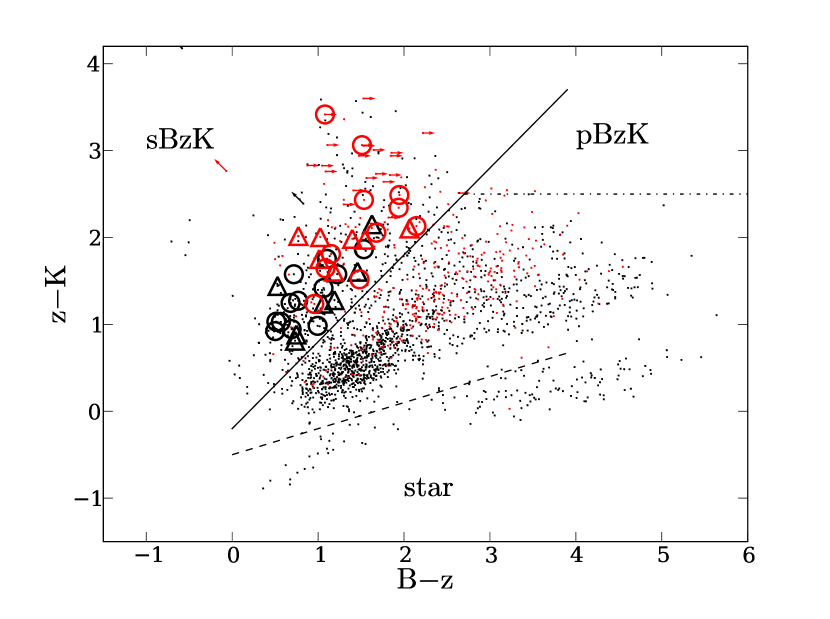
Figure 1.— BzK color-color diagram of the $K_{s}<23$ objects from the $K_{s}$-band selected catalog of the MOIRCS Deep Survey (MODS; Kajisawa et al., 2009). Red symbols show the MIPS sources listed in the public catalog (Chary et al. in preparation). The sample for the present work is denoted by circles and triangles for the objects with emission lines detected and not detected, respectively. Arrows show upper/lower limits for sBzK galaxies.

In order to select star-forming galaxies at $z\sim 2$, we apply the BzK color criterion for star-forming galaxies (sBzK; $BzK\equiv(z-K)-(B-z)>-0.2$; Daddi et al., 2004) to the $K$-selected galaxies with $K_{s}<23$ from the MODS catalog, whose limiting magnitude is $K_{s}=24.9$ ($5\sigma$, $\phi 1.2\,{\rm arcsec}$). The BzK diagram of the extracted galaxies is shown in Figure 1. $B$ and $z$ band magnitudes are measured on the F435W and F850LP images of the Advanced Camera for Surveys (ACS) on board the Hubble Space Telescope (HST) in the course of the GOODS Treasury Program (Version 1.0; Giavalisco et al., 2004). In total, 508 galaxies are identified as candidates.

We chose 37 sBzK galaxies from the candidates for the spectroscopic observation. The coordinates and photometry of the target galaxies are listed in Table 1. Although two of the sample galaxies (MODS12-0125 and MODS41-0194) are not detected in the $B$-band, we include these galaxies because their $z-K$ colors suggest that they are sBzK or passive BzK (pBzK; $BzK>-0.2\bigcap z-K>2.5$), and their photometric redshifts are consistent with the redshift range of BzK galaxies. We did not select on the basis of spectroscopic redshift, although spectroscopic redshifts were previously known for some galaxies in the present sample (Table 1).

To preferentially select actively star-forming galaxies, we put higher priority on the galaxies identified in the publicly available Spitzer MIPS source catalog (the first delivery of the Spitzer data catalog from the GOODS Legacy Project; Chary et al. in preparation). The flux limit of the catalog ($S_{24}>80\,\mu{\rm Jy}$) corresponds to $L_{TIR}\sim 4.1\times 10^{11}-3.6\times 10^{12}{\rm L}_{\odot}$ at $z=1.4-2.5$ using the infrared SED templates by Chary & Elbaz (2001); thus the galaxies in the MIPS source catalog are as luminous as (ultra-)luminous infrared galaxies. MIPS sources in the public catalog are identified with 127 of the sample galaxies (we call them sBzK-MIPS galaxies, hereafter). We selected 18 sBzK-MIPS galaxies. Furthermore, we added 19 sBzK galaxies not listed in the MIPS public catalog to the list of targets (sBzK-non-MIPS galaxies, hereafter).

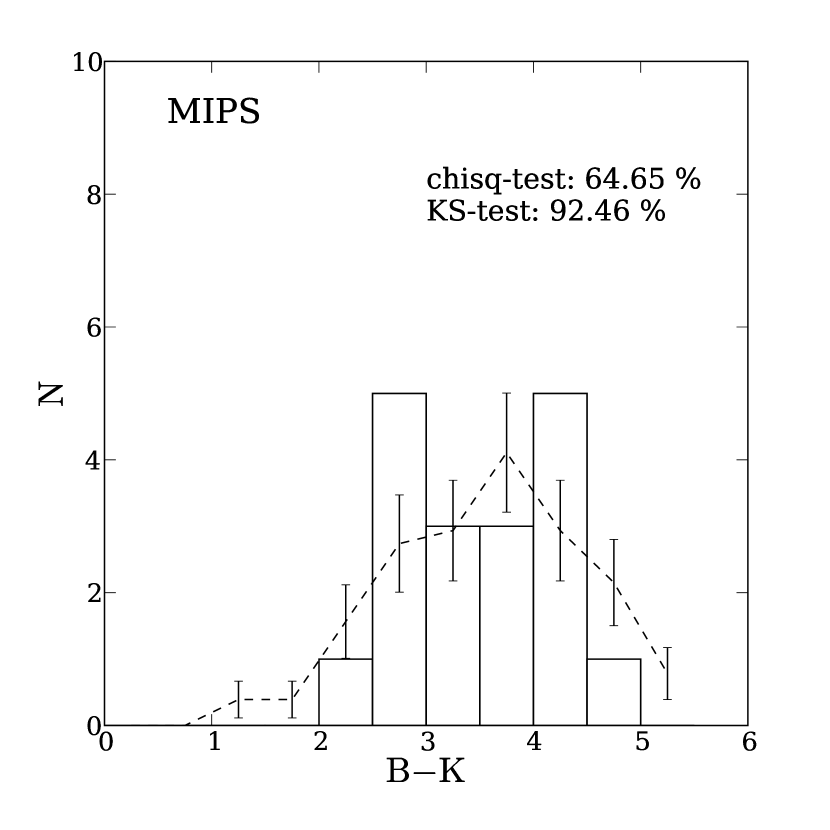
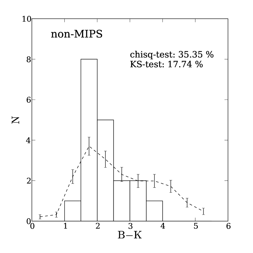
Figure 2.— $B-K$ color distribution of sBzK-MIPS (left) and sBzK-non-MIPS (right) galaxies (see text). The bar plots show our observed sample. The dashed line with error bars shows the scaled color distribution of all of the $K_{s}<23$ sBzK-MIPS and sBzK-non-MIPS galaxies, respectively. The error bars show the Poisson errors at each bins.

It is known that sBzK criterion picks out various types of star-forming galaxies and passively evolving galaxies at $1.4\leq z\leq 2.5$ (Grazian et al., 2007). In order to check that our sample represents the sBzK population, we compare the $B-K$ color distribution of our target galaxies to that of sBzK-non-MIPS and sBzK-MIPS galaxies with $K_{s}<23$ in the MODS field (Figure 2). The $B-K$ color reflects both the age and the amount of dust of a galaxy at this redshift range. Our sBzK-MIPS sample is reasonable representative of those in the field, according to both $\chi^{2}$-test (64.65 %) and Kolmorov-Smirnov (KS) test (92.46 %). On the other hand, the sBzK-non-MIPS sample is possibly biased toward blue galaxies ($\chi^{2}$-test : 35.35 %, KS-test: 17.74 %). Red sBzK-non-MIPS galaxies are relatively rare, so that the scaled number in the redder bin is too small ($\lesssim 1$) to provide robust statistics given the present sample size.

We utilize publicly available multi-wavelength data of GOODS-N to exclude possible AGN which may contaminate the optical star-formation emission. The hard X-ray luminosity at the detection limit of the Chandra Deep Field-North 2 Ms Point-Source Catalogs (Alexander et al., 2003) at $z\sim 2$ ($1\times 10^{42}\,{\rm erg\,s}^{-1}$), suggests that the emission lines of the hard X-ray detected sBzK galaxies are powered by an AGN rather than massive stars (Alexander et al., 2002). X-ray sources are identified with 62 of the 508 sBzK galaxies. We exclude these sources from the present sample. Rest-frame infrared colors are often used to identify AGN candidates using Spitzer IRAC bands (3.6 $\mu$m, 4.5 $\mu$m, 5.8 $\mu$m, and 8.0 $\mu$m) (e.g., Caputi et al., 2006b; Hayashi et al., 2009). A galaxy with emission dominated by the stellar population has a strong bump in the SED at 1.6 $\mu$m (Sawicki, 2002). We confirmed that all of the present non-X-ray galaxies have strong 1.6 $\mu$m bumps in the SED of the IRAC bands.

Table 1Properties of Galaxies Observed

ID	RA	Dec	$K_{s}$	$B-z$	$z-K$	$S_{24}$	MASK ID	$z_{\rm literature}$	$z_{\rm phot}$	$z_{\rm H\alpha}$	emission line
	(J2000.0)	(J2000.0)	(mag)	(mag)	(mag)	($\mu$Jy)
MODS11-0076	12 36 18.50	62 09 03.5	20.5	1.9	2.5	130.1	CDFN2	-	$1.48_{-0.02}^{+0.02}$	1.6731	H$\alpha$
MODS11-0094	12 36 24.29	62 08 27.9	22.2	1.0	1.2	106.8	CDFN2	-	$2.11_{-0.18}^{+0.08}$	1.9976	H$\alpha$, [OIII]
MODS11-0274	12 36 25.29	62 10 35.6	21.4	1.5	2.4	106.4	CDFN2	-	$2.10_{-0.20}^{+0.10}$	2.0808	H$\alpha$
MODS11-0299	12 36 35.64	62 09 41.4	22.9	1.2	1.3	38.6	CDFN2	-	$1.31_{-0.06}^{+0.06}$	-	-
MODS11-0390	12 36 39.37	62 10 06.6	21.8	1.5	1.5	127.2	CDFN2	-	$2.22_{-0.06}^{+0.06}$	2.3516	H$\alpha$, H$\beta$, [OIII]
MODS12-0125	12 36 11.50	62 10 33.7	21.7	$>1.5$	3.1	282.1	CDFN2	-	$2.12_{-0.12}^{+0.06}$	2.2461	H$\alpha$, [NII]
MODS12-0255	12 36 18.38	62 11 39.1	22.8	1.1	1.4	9.7	CDFN2	2.390	$2.31_{-0.06}^{+0.09}$	2.3979	H$\alpha$, H$\beta$, [OIII]
MODS21-2005	12 37 01.04	62 10 16.8	22.5	1.0	2.0	210.7	CDFN3	-	$1.98_{-0.11}^{+0.17}$	-	-
MODS21-2022	12 36 51.80	62 11 14.8	22.6	0.7	0.8	0.0	CDFN3	-	$1.47_{-0.06}^{+0.04}$	-	-
MODS21-2047	12 36 54.95	62 10 56.4	22.0	1.4	2.0	204.2	CDFN3	0.999	$2.17_{-0.06}^{+0.05}$	-	-
MODS21-2321	12 36 44.65	62 12 27.5	22.3	0.8	1.3	26.6	CDFN3	1.879	$1.56_{-0.05}^{+0.06}$	1.7341	H$\alpha$
MODS21-2612	12 37 01.07	62 10 54.3	22.1	1.9	2.3	99.0	CDFN3	-	$1.55_{-0.14}^{+0.07}$	1.5256	H$\alpha$
MODS21-4647	12 37 11.85	62 11 15.6	22.4	0.7	0.9	7.2	CDFN3	-	$1.41_{-0.04}^{+0.06}$	-	-
MODS21-5277	12 37 02.91	62 14 04.6	21.9	1.1	1.2	97.6	CDFN3	1.244	$1.24_{-0.05}^{+0.05}$	-	-
MODS21-6131	12 37 08.77	62 12 57.9	22.6	0.5	1.0	12.6	CDFN3	2.269	$2.21_{-0.52}^{+0.15}$	2.2678	H$\alpha$
MODS22-1411	12 36 26.97	62 13 17.3	22.0	1.7	2.1	148.3	CDFN2	-	$2.19_{-0.04}^{+0.08}$	2.3983	H$\alpha$, [NII], H$\beta$
MODS22-2282	12 36 21.74	62 14 52.9	22.6	0.7	1.2	12.7	CDFN1	2.200	$2.13_{-0.14}^{+0.08}$	2.2087	H$\alpha$
MODS22-2658	12 36 30.08	62 14 27.9	20.6	2.1	2.1	181.1	CDFN1	1.525	$1.37_{-0.02}^{+0.06}$	1.5246	H$\alpha$
MODS22-4194	12 36 33.67	62 15 33.0	22.8	1.0	1.0	13.4	CDFN1	2.488	$2.39_{-0.04}^{+0.04}$	2.4862	H$\alpha$
MODS22-4806	12 36 57.22	62 14 29.9	22.2	1.0	1.8	114.2	CDFN1	1.873	$1.73_{-0.10}^{+0.20}$	-	-
MODS22-5133	12 36 45.84	62 14 47.0	22.5	1.5	1.9	48.7	CDFN1	-	$1.61_{-0.06}^{+0.07}$	1.5255	H$\alpha$
MODS22-5375	12 36 50.11	62 14 01.1	22.8	0.5	1.4	69.3	CDFN1	2.231	$2.23_{-0.29}^{+0.04}$	-	-
MODS31-0033	12 37 20.05	62 12 22.8	21.9	1.2	1.8	113.3	CDFN3	2.458	$2.36_{-0.03}^{+0.08}$	2.4605	H$\alpha$, [NII], H$\beta$, [OIII]
MODS31-0129	12 37 26.43	62 13 30.3	21.1	2.1	2.1	89.2	CDFN3	-	$1.45_{-0.03}^{+0.02}$	-	-
MODS31-0199	12 37 19.39	62 16 21.1	22.5	0.7	0.9	13.8	CDFN4	1.567	$1.46_{-0.04}^{+0.04}$	1.5681	H$\alpha$
MODS32-0035	12 36 37.88	62 16 45.3	21.7	1.5	2.0	117.8	CDFN1	-	$1.45_{-0.06}^{+0.05}$	-	-
MODS32-0116	12 36 50.26	62 16 55.7	21.9	1.2	1.6	54.0	CDFN1	1.315	$1.44_{-0.10}^{+0.04}$	1.4878	H$\alpha$
MODS32-0153	12 36 53.65	62 17 24.3	21.9	0.7	1.6	71.6	CDFN1	2.186	$2.02_{-0.10}^{+0.15}$	2.1865	H$\alpha$, [OIII]
MODS32-0162	12 36 51.33	62 17 50.9	22.4	0.8	2.0	158.5	CDFN1	-	$1.83_{-0.07}^{+0.12}$	-	-
MODS41-0194	12 37 34.42	62 18 12.1	21.9	$>1.1$	3.4	118.9	CDFN4	2.241	$2.34_{-0.06}^{+0.08}$	2.2425	H$\alpha$, [OIII]
MODS41-0297	12 37 24.15	62 16 11.7	21.9	1.1	1.6	123.6	CDFN4	1.689	$1.46_{-0.04}^{+0.03}$	1.6855	H$\alpha$
MODS42-0112	12 37 16.34	62 19 20.5	22.8	0.6	1.0	19.8	CDFN4	-	$2.18_{-0.45}^{+0.05}$	2.1231	H$\alpha$, [OIII]
MODS42-0135	12 37 20.04	62 19 23.2	22.1	1.1	1.8	78.1	CDFN4	2.295	$2.36_{-0.03}^{+0.05}$	2.3049	H$\alpha$, [OIII]
MODS42-0145	12 37 24.11	62 19 04.9	22.1	0.5	0.9	32.0	CDFN4	2.094	$2.05_{-0.10}^{+0.08}$	2.0952	H$\alpha$
MODS42-0162	12 37 25.80	62 19 14.2	20.8	1.6	2.2	61.4	CDFN4	-	$1.45_{-0.11}^{+0.02}$	-	-
MODS42-0194	12 37 33.50	62 20 01.2	22.0	1.5	1.6	51.6	CDFN4	-	$1.36_{-0.05}^{+0.07}$	-	-
MODS42-0228	12 37 22.28	62 20 39.1	21.9	1.2	1.6	244.3	CDFN4	-	$1.99_{-0.17}^{+0.15}$	-	-

2.2. Observations

Table 2Summary of the observation

mask ID	R.A.	Dec.	P.A.	UT date	grism	target	exposure	seeing
	(J2000.0)	(J2000.0)	(degree)			(number)	(min)	(arcsec)
CDFN1	12 36 38.7	62 15 58	0	2007 Mar 25	HK500	10	316	0.52
CDFN2	12 36 22.3	62 10 38	249	2007 Mar 24	HK500	8	160	0.64
CDFN3	12 37 03.2	62 12 20	338	2007 Mar 26	HK500	10	310	0.68
CDFN4	12 37 21.3	62 18 28	228	2007 Mar 27	HK500	9	274	0.69

The spectroscopic observations for the selected galaxies were performed with MOIRCS (Suzuki et al., 2008) attached to the Subaru Telescope (Iye et al., 2004) during 2007 March 24–27 in the course of the near-infrared spectroscopic observation of X-ray sources (S07A-083, PI M. Akiyama). We used MOIRCS in MOS mode with the low-resolution grism (HK500), which covers 1.3–2.3 $\mu$m wavelengths. The spectral resolution is $R\sim 500$ ($\Delta v\sim 600~{}{\rm km}~{}{\rm s}^{-1}$) with 0$\farcs$8 slit width. The 37 galaxies were observed with four slit masks as shown in Table 2. One slit mask was used for each night. The total exposure time was 2.5–5 hour for each mask. The slit width was fixed to 0$\farcs$8 for targets. Most of the slit lengths were 10$\farcs$0 or longer, depending on target positions. To monitor the flux variation due to the atmospheric absorption and photon loss at the slit mask, a bright point source was observed simultaneously on each mask, except for mask CDFN3.

The FWHMs of seeing size in the $K_{s}$ band during the observations were typically $\sim 0\farcs 6$. According to the atmospheric attenuation archived in the Canada France Hawaii Telescope Web site, the conditions were photometric for the first three nights. For the forth night, thin cirrus covered the sky. The observation log is summarized in Table 2.

The observation followed the standard procedure for MOS observation with MOIRCS described in Tokoku (2007). The target acquisition was done using 6 to 7 alignment stars distributed over each slit mask. The telescope was dithered along the slit (we call it an “AB pattern”) by 3$\farcs$0, to achieve sufficient sky subtraction. The detector was read eight times in non-destructive readout mode to reduce the read out noise down to 16 $e^{-}$. The exposure time was set so that most of sky emission lines, which were used later for the wavelength calibration, were not saturated. The typical exposure times were 300–900 sec. The relative position of the alignment star against the slit mask was checked, and then the telescope pointing was adjusted every hour or two without removing the slit masks from the focal plane. The systematic guide error in one hour was measured to be $\lesssim$0$\farcs$4. At the beginning of each observing night, an A0V type star (HIP53735; $K_{s}=8.856$; Two Micron All Sky Survey point source catalog; Skrutskie et al., 2006) was observed for flux calibration with the same instrument configuration as the targets.

3. Data Reduction and Data Analysis

3.1. Data Reduction

The data reduction was made, using a semi-automatic reduction script (MOIRCS MOS Data Pipelines; MCSMDP), which follows the standard procedure of IRAF:ONEDSPEC. At first, we make a map of bad pixels; bad pixels are identified as those that show non-linearity. This includes dead (always zero count) and hot (always high count) pixels. Cosmic rays are detected by a moving block average filter using IRAF:CRAVERAGE. Each input frame for IRAF:CRAVERAGE is first divided by its dithered pair so that cosmic rays stand out behind the sky background. The cosmic-ray mask was combined with the bad pixel mask. The values of bad pixels and cosmic-ray pixels are replaced with values interpolated linearly from the pixels along the slit. Sky emission lines were subtracted using the dithered pair frames (we call the procedure “A-B subtraction”). The dome-flat frames for flat fielding were taken with the same slit mask and grism configuration as used for the observation. For the first-order distortion correction, the database for the imaging mode of MOIRCS was applied to the spectral frames. The tilt of the spectrum against the detector rows was corrected in the cases when it was measurable in the continuum of bright objects.

Next, each spectrum was cut out based on a mask design file. For wavelength calibration, OH sky emission lines were identified in each frame using a night-sky spectral atlas (Rousselot et al., 2000). Using the pixel coordinates of the sky emission lines, the sky-subtracted frames were transformed such that the sky lines aligned along the column of the frames and that the wavelength was a linear function of pixel coordinates. Background emission still remained after A-B subtraction due to time variation of OH emission during dithering observations. The residuals were subtracted by fitting with a quadratic equation along the column. Finally, all frames were weighted with the flux of the bright point source and stacked using the weighted average to obtain the final two-dimensional spectra.

The response spectra, including atmospheric transmission and the instrument efficiency, are calculated using the flux standard star to convert the observed count to an absolute flux. The data of the flux standard star is reduced to a two-dimensional spectrum in the same way for galaxy targets and then the continuum is traced with a polynomial to extract a one-dimensional spectrum with IRAF:APALL. We calculate a model spectrum of the A0V flux standard star using SPECTRUM (SPECTRUM uses Castelli & Kurucz, 2004 model). The model was scaled to $K_{s}=8.856$ and the spectral resolution of the model was degraded to $R\sim 500$ with a Gaussian kernel, so as to give the same hydrogen line width as the observed spectra. Finally, the one-dimensional spectrum of the standard star was divided by the model spectrum to obtain the response spectrum.

Emission lines are detected by visual inspection on the flux-calibrated two-dimensional spectra. The signal-to-noise ratio evaluation described later shows that visual inspection corresponds to a larger than $\sim 3\sigma$ detection. The detected emission lines were integrated along slit direction within an appropriate aperture giving the largest S/N to obtain one dimensional spectra.

3.2. Measurement of Emission Lines

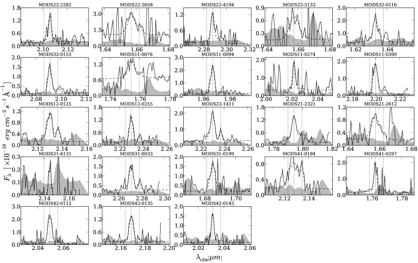
Figure 3.— [N ii]-H$\alpha$ spectra of the emission-line galaxies. Shaded region shows the size of the error as a function of wavelength. The dashed line shows the spectrum of the best-fit model. The vertical dotted lines in each panel show, from left to right, the locations of [N ii]$\lambda$6548, H$\alpha$, [N ii]$\lambda$6583.

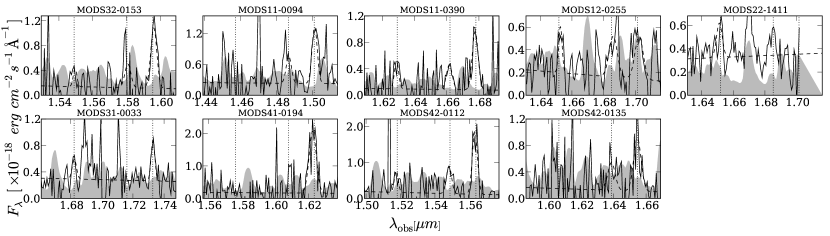
Figure 4.— Same as Figure 3, but for [O iii]-H$\beta$ spectra of the emission line galaxies with S/N$>$3. The vertical dotted lines in each panel show, from left to right, the locations of H$\beta$, [O iii]$\lambda$4959, [O iii]$\lambda$5007.

Table 3Star Formation Rates

ID	$z_{\rm H\alpha}$	$F_{\rm H\alpha}$	$L_{\rm H\alpha}$	Corrected $L_{\rm H\alpha}$	${\rm SFR}_{\rm H\alpha}$	$F_{\rm 24\,\mu m}$	$\nu L_{\rm\nu,8\,\mu m}$	${\rm SFR}_{\rm IR}$
MODS11-0076	$1.6731\pm 0.0009$	$7.1\pm 2.7$	$1.3\pm 0.5$	$29.4_{-23.4}^{+16.4}$	$144.1_{-114.8}^{+80.6}$	$130.1\pm 5.5$	$2.5\pm 0.1$	$114.6\pm 4.9$
MODS11-0094	$1.9976\pm 0.0002$	$13.9\pm 1.3$	$4.0\pm 0.4$	$31.6_{-16.0}^{+6.7}$	$155.1_{-78.5}^{+32.7}$	$106.8\pm 3.9$	$3.3\pm 0.1$	$165.6\pm 6.1$
MODS11-0274	$2.0808\pm 0.0004$	$8.0\pm 2.0$	$2.6\pm 0.6$	$47.5_{-22.4}^{+11.7}$	$232.7_{-109.8}^{+57.2}$	$106.4\pm 3.9$	$4.0\pm 0.1$	$219.8\pm 8.1$
MODS11-0390	$2.3516\pm 0.0005$	$15.1\pm 1.9$	$6.5\pm 0.8$	$202.0_{-63.8}^{+24.9}$	$989.7_{-312.7}^{+122.0}$	$127.2\pm 3.9$	$6.4\pm 0.2$	$599.4\pm 18.5$
MODS12-0125	$2.2461\pm 0.0003$	$10.0\pm 0.9$	$3.9\pm 0.3$	$42.8_{-17.7}^{+58.5}$	$209.9_{-86.6}^{+286.5}$	$282.1\pm 3.9$	$12.7\pm 0.2$	$1581.8\pm 22.0$
MODS12-0255	$2.3979\pm 0.0003$	$8.7\pm 1.1$	$3.9\pm 0.5$	$15.5_{-7.9}^{+36.1}$	$75.8_{-38.8}^{+176.9}$	$9.7\pm 9.1$	$0.5\pm 0.5$	$10.2\pm 9.6$
MODS21-2321	$1.7341\pm 0.0002$	$8.1\pm 0.9$	$1.7\pm 0.2$	$7.8_{-3.2}^{+0.8}$	$38.2_{-15.9}^{+4.0}$	$26.6\pm 3.9$	$0.6\pm 0.1$	$14.6\pm 2.2$
MODS21-2612	$1.5256\pm 0.0011$	$7.7\pm 2.2$	$1.1\pm 0.3$	$100.1_{-64.2}^{+33.8}$	$490.6_{-314.7}^{+165.8}$	$99.0\pm 3.9$	$1.7\pm 0.1$	$77.7\pm 3.1$
MODS21-6131	$2.2678\pm 0.0005$	$1.2\pm 0.3$	$0.5\pm 0.1$	$0.8_{-0.2}^{+0.2}$	$3.8_{-1.2}^{+1.0}$	$12.6\pm 3.9$	$0.6\pm 0.2$	$11.5\pm 3.6$
MODS22-1411	$2.3983\pm 0.0002$	$15.2\pm 0.9$	$6.8\pm 0.4$	$424.0_{-273.9}^{+83.3}$	$2077.4_{-1342.3}^{+408.2}$	$148.3\pm 3.9$	$7.2\pm 0.2$	$822.1\pm 21.7$
MODS22-2282	$2.2087\pm 0.0004$	$7.9\pm 1.5$	$2.9\pm 0.6$	$4.9_{-1.2}^{+2.2}$	$23.9_{-5.9}^{+10.8}$	$12.7\pm 3.9$	$0.5\pm 0.2$	$10.2\pm 3.2$
MODS22-2658	$1.5246\pm 0.0035$	$17.4\pm 4.8$	$2.6\pm 0.7$	$48.1_{-19.3}^{+35.1}$	$235.6_{-94.5}^{+171.8}$	$181.1\pm 3.9$	$2.9\pm 0.1$	$165.6\pm 3.6$
MODS22-4194	$2.4862\pm 0.0007$	$8.0\pm 2.0$	$3.9\pm 1.0$	$43.7_{-11.0}^{+21.0}$	$214.2_{-53.7}^{+103.0}$	$13.4\pm 3.9$	$0.7\pm 0.2$	$20.1\pm 5.9$
MODS22-5133	$1.5255\pm 0.0016$	$7.2\pm 4.5$	$1.1\pm 0.7$	$78.2_{-62.8}^{+51.4}$	$383.1_{-307.6}^{+251.9}$	$48.7\pm 3.9$	$0.8\pm 0.1$	$33.1\pm 2.7$
MODS31-0033	$2.4605\pm 0.0003$	$11.5\pm 1.1$	$5.5\pm 0.5$	$30.7_{-15.6}^{+3.0}$	$150.6_{-76.3}^{+14.8}$	$113.3\pm 3.9$	$6.1\pm 0.2$	$717.0\pm 24.8$
MODS31-0199	$1.5681\pm 0.0020$	$10.1\pm 2.3$	$1.6\pm 0.4$	$1.9_{-0.4}^{+1.9}$	$9.4_{-2.1}^{+9.5}$	$13.8\pm 3.9$	$0.2\pm 0.1$	$6.6\pm 1.9$
MODS32-0116	$1.4878\pm 0.0005$	$12.4\pm 2.8$	$1.7\pm 0.4$	$11.5_{-5.3}^{+5.4}$	$56.3_{-26.0}^{+26.3}$	$54.0\pm 3.9$	$0.8\pm 0.1$	$35.9\pm 2.6$
MODS32-0153	$2.1865\pm 0.0003$	$9.6\pm 0.9$	$3.4\pm 0.3$	$6.9_{-0.6}^{+4.7}$	$33.6_{-3.2}^{+22.9}$	$71.6\pm 3.9$	$2.8\pm 0.2$	$129.9\pm 7.1$
MODS41-0194	$2.2425\pm 0.0007$	$11.8\pm 5.3$	$4.5\pm 2.0$	$9.0_{-4.3}^{+9.7}$	$43.9_{-21.0}^{+47.7}$	$118.9\pm 3.9$	$4.9\pm 0.2$	$378.8\pm 12.5$
MODS41-0297	$1.6855\pm 0.0003$	$8.2\pm 1.6$	$1.6\pm 0.3$	$12.3_{-4.3}^{+5.6}$	$60.3_{-21.1}^{+27.4}$	$123.6\pm 3.9$	$2.5\pm 0.1$	$114.6\pm 3.6$
MODS42-0112	$2.1231\pm 0.0002$	$16.7\pm 1.3$	$5.6\pm 0.4$	$44.1_{-13.3}^{+9.0}$	$215.9_{-65.1}^{+43.9}$	$19.8\pm 7.3$	$0.7\pm 0.3$	$17.4\pm 6.4$
MODS42-0135	$2.3049\pm 0.0003$	$9.7\pm 1.0$	$4.0\pm 0.4$	$11.2_{-1.1}^{+11.1}$	$54.6_{-5.4}^{+54.3}$	$78.1\pm 3.9$	$3.7\pm 0.2$	$236.5\pm 11.9$
MODS42-0145	$2.0952\pm 0.0002$	$7.8\pm 1.5$	$2.5\pm 0.5$	$20.0_{-14.5}^{+3.7}$	$98.1_{-71.0}^{+18.3}$	$32.0\pm 5.2$	$1.2\pm 0.2$	$33.1\pm 5.4$

We first consider the strongest emission line as H$\alpha$. Taking account of the wavelength range where we observed and the expected redshift range of sBzK galaxies, it is the most plausible candidate for a strong emission line. The identification of H$\alpha$ is confirmed in all cases when other emission lines, such as [N ii]$\lambda\lambda$6548,6583, [O iii]$\lambda\lambda$4959,5007, and H$\beta$ are also detected at the expected wavelength. Otherwise, we check the consistency of the redshift of the H$\alpha$ emission line with that of the SED model fitting using broad-band data (see §3.4).

Although one of the conventional methods to estimate random error is to obtain the rms of the scattering of background counts at both sides of the object, the slit length for each object is not long enough. The readout noise is suppressed down to 16 $e^{-}$ by non-destructive readout mode, so that the readout noise is about 1/5 of the background noise. Because the readout noise and the photon noise of objects are negligible, we estimated the background noise by assuming that the random error is dominated by sky-background noise, which follows Poisson statistics. In parallel to the reduction of the object spectra, sky-background spectra were reduced without the background subtraction, and the Poisson error of each pixel is estimated from them. We found that the Poisson error is systematically lager than the rms error by a factor of $\sim 1.5$, though the scatter is large. The rms errors can be underestimated, because counts in the two-dimensional spectra correlate with the neighboring pixels due to the sub-pixel shift in distortion correction and wavelength calibration.

To measure the flux and central wavelength of the emission lines, we used SPECFIT (Kriss, 1994), which fits multiple emission lines and continuum simultaneously. Gaussian profiles were used for emission lines. The continuum was assumed to be a linear function of wavelength. The flux of [N ii]$\lambda 6548$ was fixed to be 1/3 of [N ii]$\lambda 6583$ flux. If H$\beta$ and/or [O iii]$\lambda\lambda$4959,5007 emission lines were detected on the two-dimensional spectra, we measured the flux in the same way. The random errors of the fluxes were estimated from the best-fit parameters of the model fitting based on the sky-background error described above. The emission lines detected with S/N$>$3 are listed in Table 1, and the spectra are shown in Figures 3 and 4. The measured flux and the redshift derived from the central wavelength of H$\alpha$ emission line are shown in Table 3.

It is difficult to accurately evaluate systematic flux error since part of the flux from the object will be lost by a slit mask; the systematic error due to the flux loss is not negligible if we measure the total flux of emission lines from slit spectroscopy. The flux loss can be caused by a variety of things, for example, a larger size of the object than the slit width, imperfect alignment of the slit mask to the target, and misalignment of the dithering direction along the slit.

First we estimated the flux loss for a point source. When a Gaussian profile with FWHM = 0$\farcs$6, which is the typical seeing during the observations, and a slit width = 0$\farcs$8 are assumed, fluxes passing through the slit are 88.4% of the integrated flux; the aperture correction factor is $\sim 1.13$. We applied this factor to the point sources observed. We found that, however, the fluxes of the point sources were still underestimated by up to $\sim 20$ %, even if we also correct the effect of the seeing size variation and pointing error, which are measured from alignment stars. This fact indicates that imperfect alignment of dithering and/or short-time variation of the seeing size during the observations can also add to the systematic error.

On the other hand, it is expected that the flux loss for extended sources varies with the size of the sources. We calculated aperture correction factors from the ratio of total flux to that expected to come in through slits, assuming that the regions emitting stellar continuum and H$\alpha$ had the same spatial distribution. The flux through a slit was measured on the $K_{s}$-band image with a rectangle of the same aperture size as for extracting one-dimensional spectrum and the same position angle of the slit, while the total flux was obtained from MAG_AUTO of SEXTRACTOR. The alignment error of the slit was estimated from the alignment stars on the slit mask. We found the median of the aperture correction factors to be $\sim 1.9$ with little dependence on the size of the objects. The rms scatter of the factor among the objects is $\pm 0.5$. We apply the median value to all objects to correct the flux loss. We checked the above aperture correction method by comparing the continuum flux derived from the corrected spectrum with total magnitude, which was measured from $K_{s}$ or $H$-band imaging data according to the redshift of each galaxy. We used 7 galaxies in the sample whose stellar continuum around the H$\alpha$ emission line was detected with sufficient S/N. We applied the aperture correction to the continuum flux, then contrasted the corrected flux with the total magnitude. The comparison shows that both results are consistent and the uncertainty in the aperture correction is within $\sim 20\,\%$.

We need to note that the assumptions on the light distribution of H$\alpha$ emission line would also cause systematic errors. The H$\alpha$ and continuum emitting regions would not always be similar for star-forming galaxies at $z\sim 2$. Studies with the integral-field spectrograph show that H$\alpha$ emission does not trace the stellar continuum in some galaxies (Swinbank et al., 2005, 2006; Kriek et al., 2007). However, this kind of check on our slit-spectroscopy sample is difficult, because both the continuum and emission lines are so faint that the light distribution along the slit is not able to be measured. As a lower limit of the aperture correction, when the H$\alpha$ emitting region is point like, the flux becomes smaller by $\sim 40\%$.

3.3. Stacking Analysis

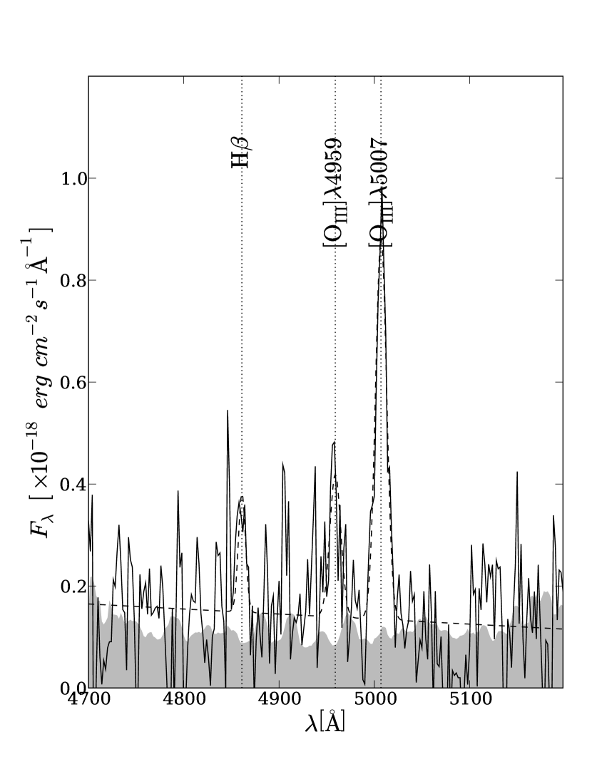
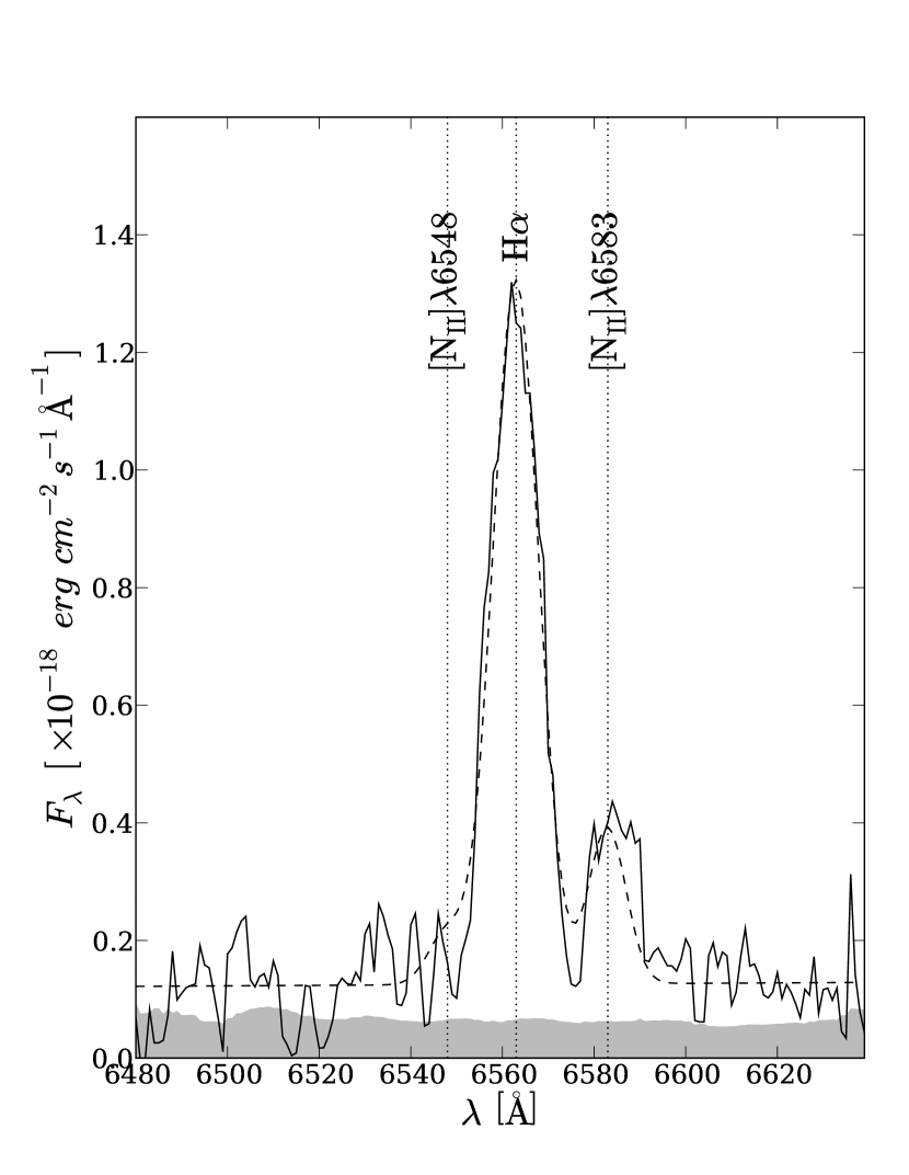
Figure 5.— Same as Figure 3, but for the stacked [O iii]-H$\beta$ (left) and the stacked [N ii]-H$\alpha$ (right) spectra. The objects which have [O iii]  and/or H$\beta$ emission are stacked for both spectra.

The flux ratios of rest-optical emission lines such as [N ii]$\lambda$6583/H$\alpha$, [O iii]$\lambda$5007/H$\beta$, and H$\alpha$/H$\beta$ provide us information on physical properties of ionized regions such as the energy sources for ionization ([N ii]/H$\alpha$ and [O iii]/H$\beta$; Baldwin et al., 1981; Veilleux & Osterbrock, 1987; Kewley et al., 2001; Kauffmann et al., 2003), the amount of dust extinction (Balmer decrement, e.g., H$\alpha$/H$\beta$; Osterbrock, 1989), and gas-phase metallicity ([N ii]/H$\alpha$; Storchi-Bergmann et al., 1994; Raimann et al., 2000; Denicoló et al., 2002; Pettini & Pagel, 2004). However, except for H$\alpha$, the emission lines of the present sample are so faint that we can not evaluate the line ratios of an individual galaxy. Therefore, we stacked the calibrated spectra in the [N ii]-H$\alpha$, and [O iii]-H$\beta$ wavelength ranges to obtain high S/N spectra, and discuss the averaged physical properties.

The stacked spectrum $\bar{F_{\lambda_{e}}}$ was calculated with

$$\bar{F_{\lambda_{e}}}=\sum\limits_{n}\frac{F_{H\alpha,0}}{F_{H\alpha,n}}F_{\lambda_{e},n}(\lambda_{e}),$$ (1)

where $F_{\lambda_{e},n}(\lambda_{e})$ and $F_{H\alpha,n}$ are the spectrum and the total H$\alpha$ flux of $\rm n_{th}$ object, respectively. The spectra were re-sampled in the rest-frame wavelength scale ($\lambda_{e}$). The fluxes were scaled with total H$\alpha$ flux, though the variety of fluxes among the samples are not large. Because our main purpose of stacking is to examine the average physical properties of galaxies from their line ratio, weighted mean (by either inverse square of noise or luminosity) is not applied; the line ratios of weighted mean flux could be biased toward strong emission line galaxies.

We selected the objects whose spectra covered the wavelengths of redshifted H$\alpha$, [N ii], H$\beta$ and [O iii]. The emission lines of the objects which had at least H$\beta$ or [O iii]  with $S/N>3$ were stacked for the measurements of the line ratios of [N ii]/H$\alpha$ and [O iii]/H$\beta$. As a result, 9 galaxies were used for the stacking. The stacked H$\alpha$-[N ii]  and H$\beta$-[O iii]  spectra are shown in Figure 5. The emission lines of the stacked spectra were fitted with a combination of the same Gaussian profiles and linear continuum measurements used in §3.2. The best-fit spectra are also shown in Figure 5. We also made stacked spectra including the objects with neither H$\beta$ nor [O iii]  detection, but the resultant line ratio was not changed.

To evaluate the effect of galaxies which would happen to have a significantly different line ratio from the others, we used a bootstrap method. We built 1000 bootstrap sets, whose galaxies were randomly selected, allowing duplicate sampling from all galaxies used in the stacking, and stacked the spectra of the galaxies in each set to derive the line ratios. We regard the 16 % and 84 % quantile of the distribution as 1$\sigma$ uncertainty in line ratio.

3.4. SED fitting

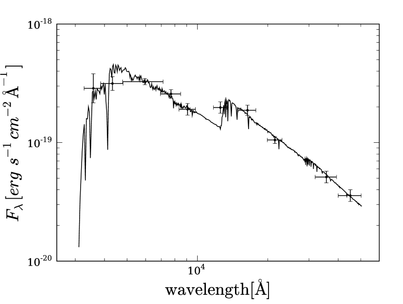
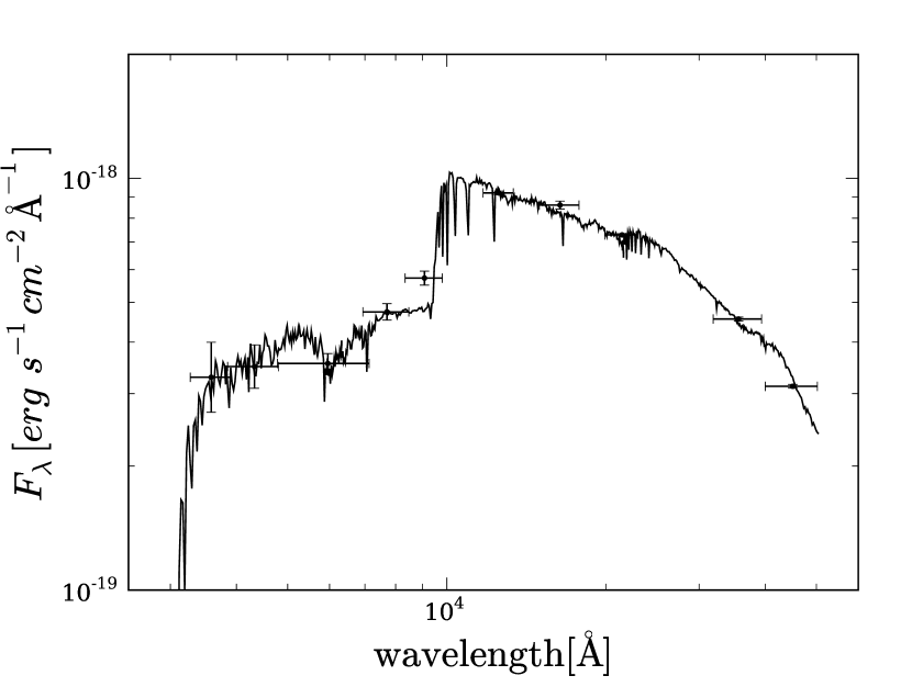
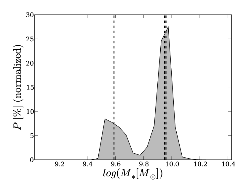
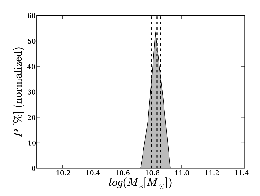
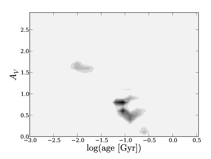
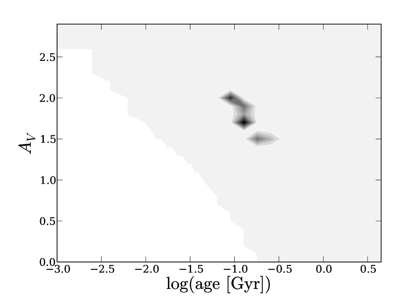
Figure 6.— Examples of best fit SEDs (top) and probability distribution against stellar mass (middle) and age versus the amount of extinction (bottom). Left and Right panels show MODS12-1025 (non-MIPS) and MODS22-2658 (MIPS), respectively. In the middle diagrams, the dashed lines show the range of 68% confidence intervals (1$\sigma$ error), and the thick dashed line shows the best-fit stellar mass.

To evaluate the properties of stellar population such as stellar mass, amount of dust extinction ($A_{V}$), and age, we use multiband photometric data from the MODS $JHK_{s}$ images and publicly available images. The publicly available images we use are: $U$(KPNO/MOSAIC; Capak et al., 2004), $BViz$ (ACS/HST; GOODS Treasury Program Version 1.0; Giavalisco et al., 2004), 3.6 $\mu$m, and 4.5 $\mu$m (IRAC/SST; DR2 of the Spitzer Legacy Science program for GOODS; Dickinson et al. in preparation). These images are deep enough to detect our galaxies with sufficient S/N and to obtain the properties of stellar population. The flux of the galaxies were obtained with ${\rm S/N}=8$ for $>80\%$ of the objects in all bands, except for $B$ (60 %) and $U$ (24 %) bands. The aperture size for photometry is set to 1$\farcs$5, which is approximately $2\times{\rm FWHM}$ of the PSF size in $K_{s}$ band. Aperture corrections were applied to each band properly (see Kajisawa et al., 2009). The contribution of H$\alpha$ emission to the flux in $K_{s}$ or $H$ band, which depends on redshift, was subtracted. The corrections are 0.01 - 0.34 mag with a median of $\sim 0.08$ mag.

We fitted the photometry data with stellar population SED models. The SED libraries of GALAXEV (Bruzual & Charlot, 2003) are used for the fitting. We adopted the libraries with metallicities of 1.0 ${\rm Z}_{\odot}$, 0.4 ${\rm Z}_{\odot}$, 0.2 ${\rm Z}_{\odot}$ and a Chabrier (2003) IMF. Exponentially declining star formation histories ($\tau$-model) are assumed: SFR $\propto e^{-t/\tau}$ with $\tau=$ 0.01, 0.02, 0.05, 0.10, 0.20, 0.50, 1.0, 2.0, and 5.0 Gyr. The starburst attenuation law of Calzetti et al. (2000) was applied to the model with 0.1 steps from $A_{V}$ = 0.0 to 3.0.

Estimations of the stellar mass are affected by the adopted IMF. Many authors employ a Salpeter (1955) IMF, which is known to overestimate stellar mass due to the steep faint-end slope of the IMF. In addition to the Chabrier (2003) IMF, we fitted the SEDs to the model with the Salpeter (1955) IMF and measured stellar mass for comparison. For our sample, the stellar mass with the Salpeter (1955) IMF is larger by a factor of $\sim 1.7$ than that with the Chabrier (2003) IMF.

Recent evolutionary population synthesis models, for example Maraston (2005), which take account of contributions of thermal-pulsating asymptotic giant branch stars to SEDs, result in changes in the inferred SED properties. We also fitted the SEDs with Maraston (2005) model and found that the model made the stellar masses smaller by a factor of $\sim 1.6$.

HYPERZ (Bolzonella et al., 2000) was used to determine best-fit SED models. The redshift for the fitting was fixed to that derived from the H$\alpha$ emission line. We derived total stellar masses of galaxies, scaling the stellar masses and SEDs with the total magnitude (MAG_AUTO) of the $K_{s}$ band. The parameter matrix, which gives a $\chi^{2}$ value for each grid of SED models, was used to evaluate the uncertainty in the model parameters. The uncertainty is obtained from the probability distributions of the parameters. For example, the probability distribution as a function of stellar mass ($P(M_{\star})$) was calculated from a minimum $\chi^{2}$ value for each stellar mass ($\chi^{2}(M_{\star})$). We determined a 68% confidence level of the distribution as 1$\sigma$ error of the parameter. The stellar population parameters and the 1$\sigma$ errors derived from the SED fitting are listed in Table 4. Some examples of the best fit SEDs and the probability distributions of stellar mass, $A_{V}$, and age are shown in Figure 6.

Table 4Stellar Population Parameters

ID	Z	$\tau$	age	mass weighted age	$A_{V}$	$M_{\star}$
	$Z_{\odot}$	Gyr	Myr	Myr		$10^{9}M_{\odot}$
MODS11-0076	0.2	0.10	$360.2_{-179.7}^{+1339.8}$	$270.4_{-152.9}^{+904.5}$	$1.8_{-0.7}^{+0.2}$	$99.9_{-2.2}^{+41.4}$
MODS11-0094	0.4	0.10	$127.8_{-63.7}^{+232.4}$	$77.2_{-11.1}^{+113.3}$	$1.2_{-0.4}^{+0.1}$	$11.9_{-0.7}^{+3.9}$
MODS11-0274	0.2	0.10	$255.0_{-127.2}^{+463.7}$	$176.7_{-61.9}^{+412.1}$	$1.7_{-0.3}^{+0.0}$	$60.4_{-2.9}^{+24.7}$
MODS11-0390	0.2	5.00	$11.5_{-0.0}^{+8.5}$	$6.0_{-0.1}^{+4.5}$	$2.0_{-0.2}^{+0.0}$	$12.3_{-0.9}^{+2.1}$
MODS12-0125	0.2	2.00	$3500.0_{-2991.2}^{+0.0}$	$2430.2_{-2050.1}^{+0.0}$	$1.4_{-0.3}^{+0.5}$	$181.1_{-81.1}^{+0.0}$
MODS12-0255	0.4	0.02	$90.5_{-77.3}^{+37.3}$	$82.1_{-75.5}^{+25.0}$	$0.8_{-0.4}^{+0.7}$	$9.1_{-5.2}^{+0.0}$
MODS21-2321	0.4	0.02	$90.5_{-0.0}^{+90.0}$	$82.1_{-0.9}^{+52.7}$	$0.9_{-0.3}^{+0.0}$	$9.0_{-0.8}^{+0.6}$
MODS21-2612	0.4	0.01	$36.0_{-6.0}^{+472.8}$	$27.0_{-6.6}^{+155.0}$	$2.6_{-0.5}^{+0.1}$	$10.7_{-0.5}^{+13.3}$
MODS21-6131	0.2	0.01	$90.5_{-0.0}^{+37.3}$	$91.5_{-0.3}^{+15.6}$	$0.3_{-0.1}^{+0.0}$	$8.3_{-0.3}^{+0.2}$
MODS22-1411	0.2	5.00	$20.0_{-6.8}^{+19.0}$	$10.5_{-3.7}^{+8.6}$	$2.4_{-0.6}^{+0.1}$	$19.8_{-2.8}^{+11.8}$
MODS22-2282	0.2	0.01	$127.8_{-0.0}^{+127.2}$	$117.8_{-10.6}^{+86.4}$	$0.3_{-0.1}^{+0.2}$	$7.5_{-0.1}^{+1.8}$
MODS22-2658	1.0	0.01	$127.8_{-37.3}^{+52.7}$	$117.8_{-26.6}^{+52.0}$	$1.7_{-0.2}^{+0.3}$	$68.4_{-5.3}^{+4.1}$
MODS22-4194	1.0	5.00	$10.0_{-0.0}^{+1.5}$	$5.2_{-0.1}^{+0.8}$	$1.4_{-0.0}^{+0.2}$	$3.4_{-0.0}^{+1.4}$
MODS22-5133	1.0	0.50	$22.9_{-7.8}^{+29.6}$	$11.5_{-2.4}^{+23.9}$	$2.5_{-0.4}^{+0.1}$	$3.7_{-0.3}^{+2.5}$
MODS31-0033	0.4	0.05	$180.5_{-0.0}^{+328.3}$	$135.6_{-18.1}^{+211.1}$	$1.0_{-0.4}^{+0.0}$	$35.0_{-2.6}^{+8.7}$
MODS31-0199	1.0	0.10	$360.2_{-232.4}^{+0.0}$	$270.4_{-163.3}^{+0.0}$	$0.1_{-0.0}^{+0.4}$	$7.0_{-2.3}^{+0.0}$
MODS32-0116	0.2	1.00	$1015.2_{-655.0}^{+1284.8}$	$676.0_{-400.5}^{+554.3}$	$1.1_{-0.3}^{+0.2}$	$19.9_{-5.5}^{+2.5}$
MODS32-0153	0.2	0.10	$360.2_{-179.7}^{+148.6}$	$270.4_{-135.5}^{+76.3}$	$0.4_{-0.0}^{+0.3}$	$20.5_{-0.1}^{+3.5}$
MODS41-0194	0.2	0.50	$2600.0_{-1584.8}^{+0.0}$	$2261.9_{-1328.7}^{+0.0}$	$0.4_{-0.1}^{+0.4}$	$80.9_{-13.3}^{+6.2}$
MODS41-0297	0.4	2.00	$1015.2_{-887.4}^{+418.8}$	$623.7_{-494.9}^{+37.0}$	$1.2_{-0.2}^{+0.2}$	$28.5_{-11.5}^{+0.0}$
MODS42-0112	0.2	0.05	$17.4_{-5.9}^{+12.6}$	$9.7_{-3.0}^{+6.2}$	$1.2_{-0.2}^{+0.1}$	$2.2_{-0.3}^{+0.4}$
MODS42-0135	0.2	0.02	$180.5_{-90.0}^{+74.5}$	$160.5_{-154.9}^{+43.6}$	$0.6_{-0.0}^{+0.4}$	$19.5_{-2.1}^{+3.5}$
MODS42-0145	0.2	0.02	$11.5_{-0.0}^{+116.3}$	$6.6_{-0.0}^{+80.5}$	$1.2_{-0.7}^{+0.0}$	$4.3_{-0.1}^{+6.9}$

4. Results

4.1. Properties of H$\alpha$ Emission Lines

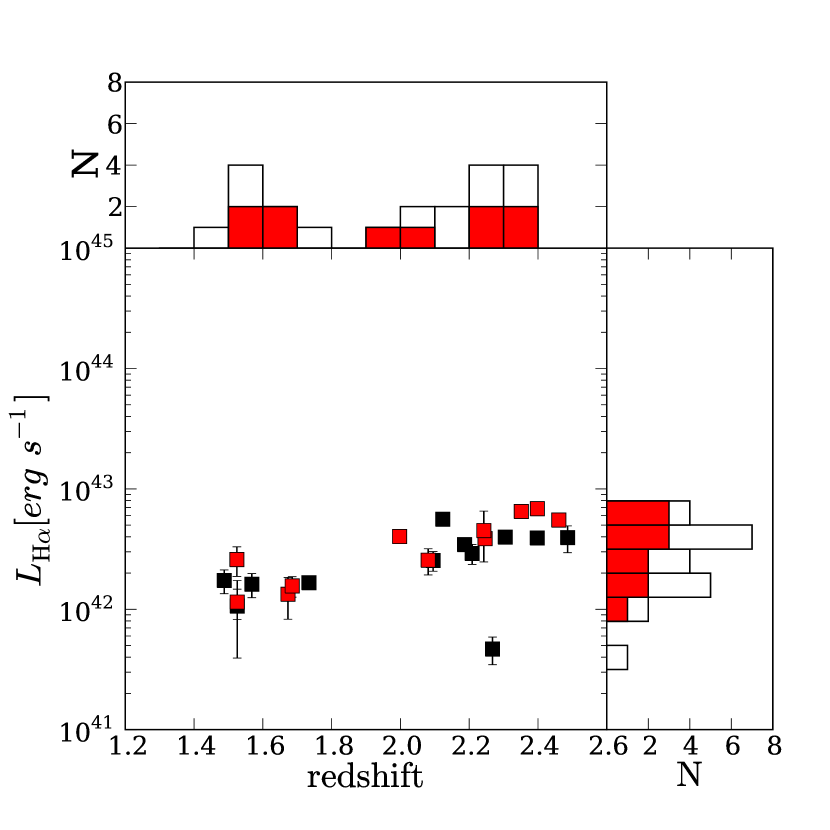
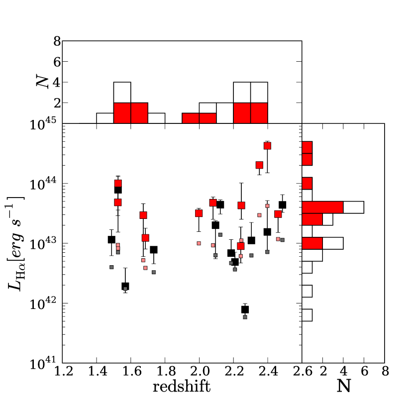
Figure 7.— Luminosity of H$\alpha$ emission lines and redshift distribution of the H$\alpha$-detected sBzK galaxies before (left) and after (right) extinction correction. Red and black symbols show sBzK-MIPS and sBzK-non-MIPS galaxies, respectively. In the right figure, small symbols show the results of the equal-extinction case correction to the stellar continuum.

H$\alpha$ emission lines are detected from 23 out of the 37 galaxies (62 %). The detection rate does not depend on the mid-IR flux. The rate for sBzK-MIPS and sBzK-non-MIPS galaxies are 11/18 (61 %) and 12/19 (63 %), respectively.

The spectroscopic redshifts are consistent with their photometric redshifts in the MODS catalog (Kajisawa et al., 2009); the median value of the relative errors is $\left<dz\right>\sim-0.026$ with a scatter of 0.035, where $dz\equiv(z_{\rm phot}-z_{\rm H\alpha})/(1+z_{\rm H\alpha})$. The spectroscopic redshifts are newly determined for 10 galaxies. Out of the remaining 13 galaxies with spectroscopic redshifts in the literature (Cohen, 2001; Cohen et al., 2000; Dawson et al., 2001; Wirth et al., 2004; Cowie et al., 2004; Treu et al., 2005; Chapman et al., 2005; Reddy et al., 2006b; Barger et al., 2008), two galaxies have slightly different spectroscopic redshift. MODS32-0116 has $z_{\rm H\alpha}=1.488$ ($z_{\rm literature}=1.315$) and MODS21-2321 has $z_{\rm H\alpha}=1.734$ ($z_{\rm literature}=1.879$).

The left panel of Figure 7 shows the apparent H$\alpha$ luminosity and the redshift distribution of the H$\alpha$-detected sBzK galaxies. The galaxies lie at redshifts between 1.49 and 2.49 with a median of 2.12. The redshift distribution is consistent with that expected for BzK galaxies ($1.4\lesssim z\lesssim 2.5$; Daddi et al., 2004). The lack of galaxies at $1.8<z<2.0$ is due to an atmospheric absorption band between $H$ and $K$ bands.

The luminosity distances of these objects are calculated with their redshifts measured using the H$\alpha$ emission lines. The fluxes of H$\alpha$ emission lines ($F_{H\alpha}$) range between 1 and 17 $\times 10^{-17}\,{\rm ergs\,s}^{-1}\,{\rm cm}^{-2}$, which corresponds to an H$\alpha$ luminosity ($L_{H\alpha}$) of 0.5 to 7.0 $\times 10^{42}\,{\rm ergs\,s}^{-1}$. $F_{H\alpha}$ and $L_{H\alpha}$ are listed in Table 3.

Possible reasons for non-detections of emission lines from the remaining 14 galaxies are; (1) their H$\alpha$ emission lines are too faint for the present observations; (2) the redshift of those galaxies are out of the $1.2\lesssim z\lesssim 2.5$ range, where the grism (HK500) we used covers the H$\alpha$ wavelength; (3) the galaxies lie at the redshift where H$\alpha$ emission line falls on strong sky emission lines or atmospheric absorption bands. Because the photometric redshifts and the errors of the galaxies with emission lines undetected are at $1.2<z<2.5$, the second possibility is unlikely except for MODS21-2047, whose $z_{\rm literature}$ is 0.999. In order to check the third possibility, we calculate the detection limit of H$\alpha$ emission as a function of redshift using the sky background noise and the response spectrum. A Gaussian profile is assumed for H$\alpha$ with $\rm FWHM=540\,km\,s^{-1}$, which corresponds to the wavelength resolution of the HK500 grism with a 0$\farcs$8 slit width. Provided that H$\alpha$ emitters have a uniform redshift distribution at $1.4\leq z\leq 2.5$ and an apparent H$\alpha$ luminosity of $1.8\times 10^{42}\,{\rm ergs}\,{\rm s}^{-1}$, which corresponds to the 84 % quantiles of the distribution of apparent H$\alpha$ luminosity, the expected detection rate of the H$\alpha$ emission line with ${\rm S/N}>4$ is 87.7 %, which corresponds to $\sim 32$ objects: objects at $1.8\lesssim z\lesssim 2.0$ are rarely detected. Therefore, for 5 of the observed samples, H$\alpha$ emission lines are undetected due to the strong sky emission lines or atmospheric absorption bands, while the remaining 9 galaxies have smaller SFR and/or larger attenuation than the galaxies with emission line detection.

4.2. [O iii]$\lambda$5007/H$\beta$ and [N ii]$\lambda$6583/H$\alpha$ Line Ratios

Diagnostic diagrams based on optical emission-line ratios are commonly used to determine the energy source of ionization. Possible sources are massive stars, AGNs and energetic shocks (Baldwin et al., 1981; Veilleux & Osterbrock, 1987). In this paper, we use H$\alpha$ luminosity as an indicator of SFR, assuming that its energy source is massive stars. We excluded AGN candidates from the sample using multi-wavelength data (see §2.1). In addition to these diagnostics, we use optical emission-line ratios to determine the energy sources of the present emission line objects.

In Figure 8, we plotted [O iii]$\lambda$5007/H$\beta$ and [N ii]$\lambda$6583/H$\alpha$ line ratios of the stacked spectra and the galaxy with the four emission lines detected (MODS31-0033). Results for $\sim 347000$ galaxies from SDSS DR6 (Adelman-McCarthy et al., 2008) and local emission line galaxies (Moustakas & Kennicutt, 2006) are also shown. A classification line empirically determined from the SDSS objects (Kauffmann et al., 2003) and a theoretically determined classification line (Kewley et al., 2001) are also shown. Emission-line galaxies located below and to the left of the lines are expected to have massive stars for their energy sources. The distribution of local SDSS galaxies exhibits the two expected sequences: the populations below (star-forming galaxies) and above (AGNs) the solid line.

The emission line of the stacked sample place it on the theoretical line, while MODS31-0033 is located to the lower left of the empirical line. Our results are located above the sequence of local star-forming galaxies, closer to the AGN sequence. In fact, a similar offset is seen in star-forming galaxies at $z\sim 2$ (Erb et al., 2006a; Kriek et al., 2007). One possible reason for the offset is a higher electron density and a harder ionizing spectrum than for local star-forming galaxies (Erb et al., 2006a).

We note that AGNs can be also identified based on [O iii]-H$\alpha$ line ratios for objects without an H$\beta$ detection. AGNs typically have [O iii]/H$\beta$ $\gtrsim 3$ on Figure 8. On the other hand since the H$\alpha$/H$\beta$ line ratio must be $\sim 3$ (the Balmer decrement) or larger (if there is a significant dust extinction) the [O iii]-H$\alpha$ line ratio of an AGN candidate will be larger than 1. Only one object (MODS41-0194) has [O iii]-H$\alpha$ $>1$ (1.67). When we exclude MODS41-0194 from the stacking, the stacked line ratios slightly move below the empirical line (Figure 8). We regard this object as a possible candidate of AGN in the later discussion.

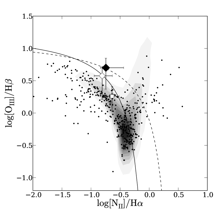
Figure 8.— [N ii]-H$\alpha$ and [O iii]-H$\beta$ line ratios. The black diamond shows the line ratios of the stacked spectra, while the white diamond is the stacked spectra with MODS41-0194 (a possible AGN candidate; see text) excluded. The open square is MODS31-0033, in which the four emission lines are detected. The contours in gray scale show the distribution of $\sim 347000$ objects from SDSS DR6, while the black dots show local starburst galaxies analyzed by Moustakas & Kennicutt (2006). The solid line is the empirically determined classification line derived for the SDSS objects by Kauffmann et al. (2003). Objects below and to the left of this line are normal starburst galaxies. The dashed line is the classification boundary theoretically determined by Kewley et al. (2001).

4.3. Extinction

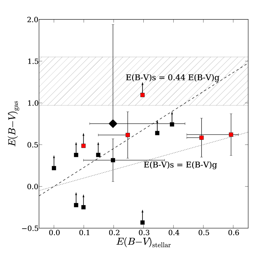
Figure 9.— Comparison of dust extinction derived from an SED fit to that derived from the Balmer decrement. The black diamond shows the stacked spectrum. Red and black squares show sBzK-MIPS and sBzK-non-MIPS galaxies, respectively. Squares with error bars are the galaxies with an H$\beta$ emission line detected (MODS11-0390, MODS12-0255, MODS22-1411, MODS31-0033), while those with upper arrows are the galaxies with an H$\beta$ upper limit (3$\sigma$). The hatched region shows the 3$\sigma$ detection limit of H$\beta$ estimated from H$\alpha$ flux. The height of the region is calculated from the 68% distribution of the H$\alpha$ fluxes. The dotted and dashed lines illustrate the equal-extinction case and the relation given by Calzetti (2001) (Equation 3), respectively.

In order to evaluate SFR from intrinsic H$\alpha$ luminosity, the extinction due to interstellar dust needs to be corrected. Moreover, the samples are expected to have large amounts of dust, because about half of the present galaxies are luminous infrared galaxies, in which strong infrared emission is thought to originate from dust thermal emission.

The extinction of emission lines in star-forming regions can be estimated with the reddening of the Balmer decrement through an extinction curve. The intrinsic line ratios of the Balmer emission lines are nearly constant with respect to electron temperature of ionized gas. The amount of reddening is estimated from the ratio of the attenuated-to-intrinsic Balmer line ratio,

$$E(B-V)_{\rm gas}=\frac{2.5}{k(\lambda_{H\alpha})-k(\lambda_{H\beta})}\log\frac{F_{i}^{\lambda_{H\alpha}}/F_{i}^{\lambda_{H\beta}}}{F_{o}^{\lambda_{H\alpha}}/F_{o}^{\lambda_{H\beta}}},$$ (2)

where “i” and “o” denote intrinsic and observed flux, respectively, and $k(\lambda)$ is an extinction curve. We assume Calzetti et al. (2000) law for $k(\lambda)$.

The Balmer decrement method can only be applied to the 14 galaxies at $z\gtrsim 1.9$ in the present sample, because the H$\beta$ wavelength is not covered by the HK500 grism for galaxies at lower redshift. Both H$\alpha$ and H$\beta$ are detected in four galaxies (MODS11-0390, MODS12-0255, MODS22-1411, MODS31-0033), so that $E(B-V)_{\rm gas}$ is estimated using the above equation. For the rest of the sample, lower limits on the $E(B-V)_{\rm gas}$ are evaluated using H$\beta$ emission-line upper limits. The resultant $E(B-V)_{\rm gas}$ values are $\gtrsim 0.5$. We also used the stacked spectrum to measure the average amount of reddening and found it to be $E(B-V)_{\rm gas}=0.75^{+1.19}_{-0.02}$.

We estimate the amount of reddening for the ionized gas from the SED fitting and apply these extinction corrections to the H$\alpha$ luminosities for all of the galaxies. Figure 9 shows the comparison between the amounts of reddening derived from the Balmer decrement and SED fitting. Our result shows that the gas is more attenuated than the stars. From SED fitting, the amount of reddening for stars in the samples used for stacking are found to be $E(B-V)_{{\rm stellar}}=0.20^{+0.24}_{-0.08}$, thus $E(B-V)_{{\rm stellar}}/E(B-V)_{{\rm gas}}\sim 0.26^{+0.42}_{-0.10}$. It should be noted that the galaxies which we used to determine the relation suffer relatively less attenuation since we would not be able to detect H$\beta$ emission in the more highly attenuated galaxies. The hatched region in the figure also shows the lower limit of $E(B-V)_{\rm gas}$ corresponding to the 3$\sigma$ detection limit of H$\beta$. The height of the region calculated from the 68% distribution of the observed H$\alpha$ fluxes.

From studies of local starburst galaxies, it is known that ionized gas is more attenuated than stars (Calzetti et al., 2000; Calzetti, 2001). The difference is thought to be caused by changes in the geometry of the ionized gas and stars in a typical galaxy. Calzetti (2001) give the relation between the color excess observed for gas and stars:

$$E(B-V)_{{\rm stellar}}=0.44E(B-V)_{{\rm gas}}.$$ (3)

This relation is shown with the dashed line in Figure 9. Our stacked result is consistent with the equation within errors. On the other hand, H$\beta$ detected galaxies are also consistent with the case that extinction for gas and stars is equal (defined as “equal extinction”, hereafter), though these galaxies would lie at the lower end of reddening as noted above. We, therefore, employ Equation 3 as an averaged nature of dust extinction to correct for the effect of dust extinction on the emission lines and compare these with that calculated assuming equal extinction. We discuss the reliability of the application of these extinction correction further in the §5.1.

The right panel of Figure 7 shows the luminosity of the H$\alpha$ emission lines of the galaxies after the extinction is corrected. The extinction correction factor of our samples ranges from 1.2 to 87, resulting in a wider spread in extinction corrected H$\alpha$ luminosities ($\sim 0.6$ dex for the Calzetti (2001) relation and $\sim 0.4$ dex for equal extinction) than in the apparent H$\alpha$ luminosities ($\sim 0.3$ dex). This result indicates that proper extinction correction is important to reliably calculate the intrinsic H$\alpha$ luminosity.

4.4. Star Formation Rate and Stellar Mass

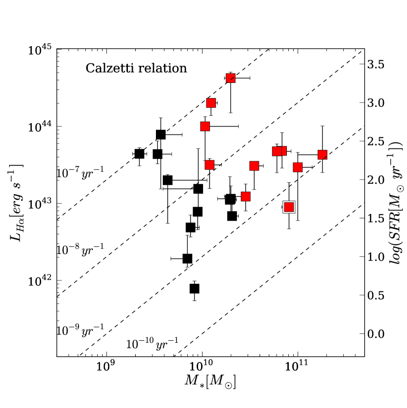
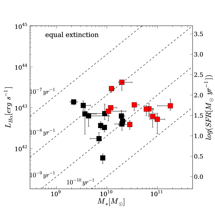
Figure 10.— H$\alpha$ luminosity with extinction corrected using the Calzetti relation (left) and the equal-extinction case (right) as a function of stellar mass derived from SED fitting. Red and black squares show sBzK-MIPS and sBzK-non-MIPS galaxies, respectively. MODS41-0194, which is the possible AGN candidate discussed in §4.2, is denoted by an open square. ${\rm SFR}_{H\alpha}$ (the right axis) is calculated by Equation. 4. The dashed lines indicate SSFRs.

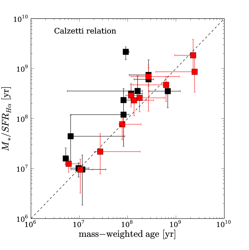
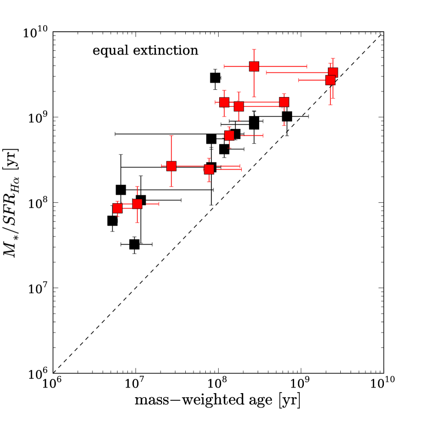
Figure 11.— SSFR age (${\rm SSFR}^{-1}$) with extinction corrected using the Calzetti relation (left) and the equal-extinction case (right) as a function of mass weighted age. The dashed line shows the equal age. Symbols are same as Figure 10.

To convert the extinction-corrected H$\alpha$ luminosity to SFR, we derive a relation between them using stellar population synthesis models, following Kennicutt (1998). We employ GALAXEV models (Bruzual & Charlot, 2003) with the Chabrier (2003) IMF and the same parameters as used in §3 to calculate ionizing photons ($N_{{\rm Ly}}$). $N_{{\rm Ly}}$ is converted to $L(H\alpha)$ based on a case-B recombination model (Osterbrock, 1989). If a constant SFR model and solar metallicity are assumed, the $L(H\alpha)$-SFR relation with an age older than 20 Myr is given by,

$${\rm SFR}(H\alpha)({\rm M}_{\odot}~{}{\rm yr}^{-1})=4.9\times 10^{-42}L(H\alpha)({\rm erg}~{}{\rm s}^{-1}).$$ (4)

Using this equation, we derived the SFR with extinction-corrected H$\alpha$ luminosity. The result is listed in Table 3. The SFR estimate is larger by a factor of $\sim 1.5$, if the Salpeter (1955) IMF is adopted.

The stellar masses derived from the SED fitting are compared with the SFRs calculated using both extinction correction approaches in Figure 10. For the extinction correction using the Calzetti (2001) relation, the SFRs range from 10 to several hundreds ${\rm M}_{\odot}\,{\rm yr}^{-1}$. Some massive galaxies ($\sim 10^{11}\,{\rm M}_{\odot}$) and a significant fraction of low mass galaxies show SFR larger than $100\,{\rm M}_{\odot}\,{\rm yr}^{-1}$. As a result, there is no clear correlation between SFR and stellar mass. The present sample contains many sBzK-MIPS galaxies, whose SFRs are expected to be high. Although sBzK-MIPS galaxies lie at the massive and high SFR end of the distribution, there still exist low-mass and high-SFR galaxies among sBzK-non-MIPS galaxies.

The specific SFR (SSFR), which is the SFR divided by stellar mass, is one of the indicators showing the level of star formation; higher SSFR indicates that a galaxy is accumulating large stellar mass compared to its own stellar mass on a short timescale. In Figure 10, SSFR is depicted by dashed lines. SSFR does not depend on MIPS detection but on stellar mass. There exist actively star-forming galaxies (${\rm SSFR}>10^{-8}\,{\rm yr}^{-1}$) among the less-massive galaxies, while the SSFR of massive galaxies ($\gtrsim 10^{10}\,{\rm M}_{\odot}$) is nearly constant ($\sim 2\times 10^{-9}\,{\rm yr}^{-1}$). It can imply that some low mass galaxies at $z\sim 2$ are actively forming stars.

On the other hand, for the SFRs corrected assuming the equal-extinction case, the SFRs and SSFRs of the high-SSFR galaxies become lower, but they still have higher SSFR when compared to other galaxies. The SSFR of the original high-SSFR galaxies become ${\rm SSFR}>3.5\times 10^{-9}\,{\rm yr}^{-1}$. Consequently, there is still no correlation between them. The distribution of SFRs is nearly constant ($\sim 30\,{\rm M}_{\odot}\,{\rm yr}^{-1}$).

The possible AGN candidate (MODS41-0194; denoted by a open square) shows lower SFR than other galaxies with similar stellar masses. We note that this object does not change our findings of no correlation between SFR and stellar mass and low mass galaxies with active star formation.

The inverse of SSFR (SSFR age) gives the estimated age for a galaxy to build up all of its stellar mass with the current SFR. On the contrary, mass-weighted age, which is calculated by integrating the ages of stars weighted by SFR at that time, is an indicator of the average age of the stars in a galaxy. The mass-weighted age is given from integration of the star formation history of galaxy as

$$\tilde{T}(t)=\frac{\int^{t}_{0}\phi(t^{\prime})\times(t-t^{\prime})dt^{\prime}}{\int^{t}_{0}\phi(t^{\prime})dt^{\prime}},$$ (5)

where $\phi(t)$ is the SFR at age t. Comparing the two ages, we can roughly check consistency between the SED fitting result and the SFR estimated from extinction corrected H$\alpha$ luminosity. The comparison between the SSFR age for the both cases of extinction correction and mass-weighted age of our sample is shown in Figure 11. For extinction correction with the Calzetti (2001) relation, the SSFR ages agree with the mass-weighted ages to within 1 $\sigma$ error; a galaxy with a higher SSFR has a younger stellar population. This fact suggests that the majority of the stellar mass for the galaxies in our emission line samples were formed in a recent starburst. On the other hand, for the extinction correction assuming the equal extinction case, the ages of stars are young compared to the SFR especially for high-SSFR galaxies. In this case the galaxies must have experienced much more active star formation in the recent past and terminated the star formation in a very short timescale ($\lesssim 10\,$Myr).

5. Discussion

5.1. Extinction Correction and Star Formation Rate

The median value of the reddening derived from the SED fitting is $E(B-V)_{\rm stellar}=0.42,\,0.21$ ($A_{V}=1.7,\,0.85$) for sBzK-MIPS and sBzK-non-MIPS galaxies, respectively. Both values are relatively larger than those for local galaxies (e.g., $\left<A_{V}\right>_{\rm median}\sim 0.43$ for $r$-band selected SDSS galaxies; Kauffmann et al., 2003). The extinction corrections are key to the discussion on the luminosities of H$\alpha$ emission line, and thus the SFRs and SSFRs; larger extinction correction makes extinction-corrected SFR and SSFR larger. In this section, we discuss the reliability of our extinction correction through comparisons of the H$\alpha$ SFRs with other SFR indicators, and the reason why the higher SSFR galaxies are found by our observation.

5.1.1 UV Luminosity

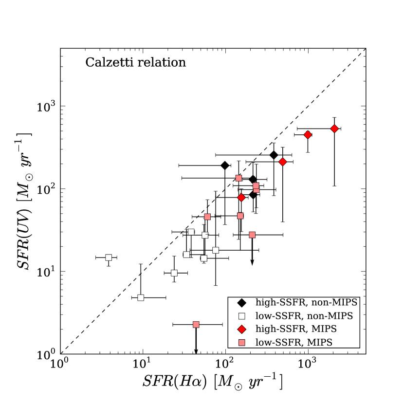
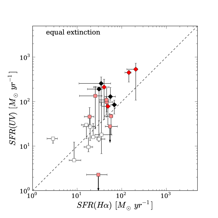
Figure 12.— (left) Comparison of SFRs inferred from H$\alpha$ luminosity (SFR(H$\alpha$)) and UV luminosity (SFR(UV)). Diamonds and squares are high-SSFR (${\rm SSFR}>10^{-8}\,{\rm yr}^{-1}$) and low-SSFR (${\rm SSFR}<10^{-8}\,{\rm yr}^{-1}$ galaxies, respectively. Red symbols are MIPS-selected samples. The SFR(UV) is calculated by Equation 6, with UV luminosity, which is measured with $\phi$1$\farcs$5 in $B$-band with an aperture correction obtained by $K_{s}$-band total magnitude. The dust extinction is corrected with that derived from SED fit. (right) Same as left, but Calzetti (2001) relation is not used for extinction correction for H$\alpha$ luminosity.

The UV continuum is used as a SFR indicator, because the stellar continuum at 1500-2800 Å is sensitive to emission from massive stars. We compare the SFRs with those estimated from the UV continuum. We calculate a relation between UV continuum at $\lambda=1500$ Å, $L_{\nu,1500\AA}$, and SFR as for Equation 4. $L_{\nu,1500\AA}$ is measured from the SED templates of GALAXEV with the same parameters as in §4.4 with the $B$-band filter of ACS/HST redshifted to $z=2$. The relation is given by,

$${\rm SFR(UV)}(M_{\odot}~{}{\rm yr}^{-1})=7.50\times 10^{-29}L_{\nu,1500\AA}({\rm erg}~{}{\rm s}^{-1}~{}{\rm Hz}^{-1}).$$ (6)

For our samples, $L_{\nu,1500\AA}$ is measured with $\phi$1$\farcs$5 in $B$-band with an aperture correction obtained from the $K_{s}$-band total magnitude. The dust extinction is corrected with that derived from the SED fit.

The comparison between SFR(H$\alpha$) and SFR(UV) is shown in Figure 12. For the equal-extinction case, the SFR(H$\alpha$) is underestimated for the galaxies with higher SFR(UV). On the other hand, using the Calzetti (2001) relation the SFR(H$\alpha$) and SFR(UV) are roughly consistent for a broad range of SFR, but are systematically larger by 0.3 dex for both sBzK-MIPS and sBzK-non-MIPS galaxies.

We note that the luminosity ratio of the UV continuum to H$\alpha$ varies with the population of a galaxy. For example, because the UV continuum is contaminated by less massive stars than stars emitting ionizing photon, galaxies populated by younger massive stars are more luminous in H$\alpha$. For our template, the ratio is larger by factor $\sim 3$ for age $\lesssim 10\,$Myr and becomes constant for age $\gtrsim 100\,$Myr. In fact, high-SSFR galaxies have a mass-weighted age $\lesssim 100\,$Myr. If a top-heavy IMF is assumed, moreover, the ratio gets larger, so that more ionizing photons are emitted than UV continuum.

5.1.2 MIPS Flux

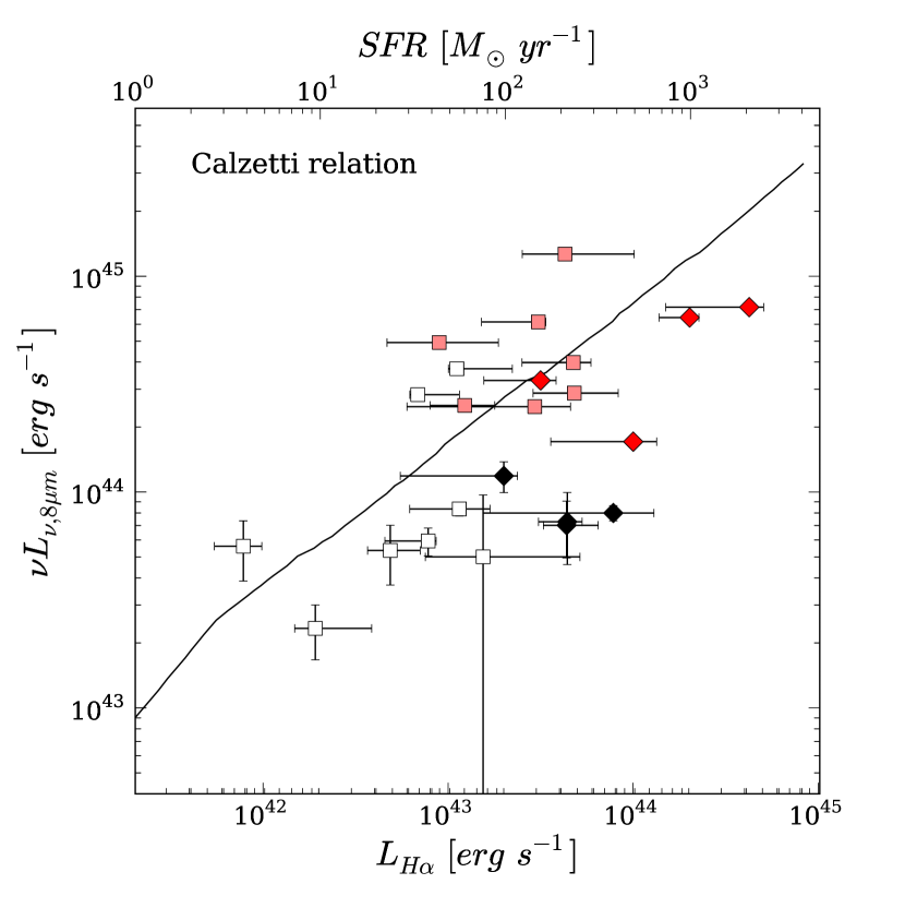
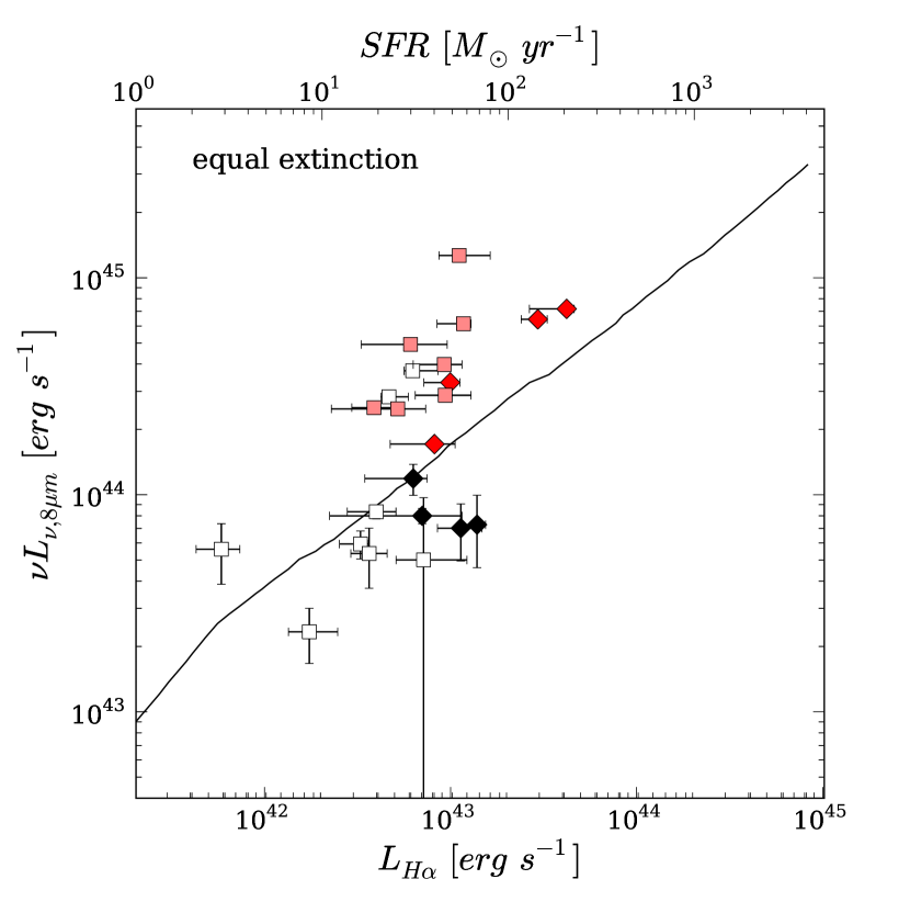
Figure 13.— (left) Comparison of H$\alpha$ emissions with rest-8 $\mu$m luminosity. Symbols are same as in Figure 12. The 24 $\mu$m fluxes are measured from a Spitzer MIPS image (Dickinson et al. in preparation) with IRAF/DAOPHOT package (Stetson, 1992) (see text). The solid line shows the expected relation between $\nu L_{\nu,8\mu m}$ and H$\alpha$ luminosity (see text). The error bars of $\nu L_{\nu,8\mu m}$ are estimated from photometric error of 24 $\mu$m flux and the residual of fitting. (right) Same as left, but Calzetti (2001) relation is not used for extinction correction for H$\alpha$ luminosity.

In order to examine the reliability of the extinction corrections further, we compare the SFR(H$\alpha$) estimates with those derived from the thermal infrared luminosities (SFR(IR)), because the infrared luminosity is an SFR indicator almost unaffected by dust extinction. We use the rest-8 $\mu$m luminosity ($\nu L_{\nu,8\mu m}$) derived from the MIPS 24 $\mu$m flux as representative of the thermal infrared luminosity. Independently from the public catalog, the 24 $\mu$m fluxes of the present galaxies are measured using the $Spitzer$ MIPS image (Dickinson et al. in preparation) with the IRAF/DAOPHOT package (Stetson, 1992) for both sBzK-MIPS and sBzK-non-MIPS samples. Some galaxies have 24$\mu$m fluxes severely contaminated by nearby bright 24$\mu$m sources because of the large PSF of MIPS (${\rm FWHM}\sim 5\farcs 4$). In order to reduce the effect of the contamination, the fluxes are measured by fitting crowded objects simultaneously with the PSF measured from isolated point sources. The objects are centered using the $K_{s}$-band light distribution. The photometric error is estimated on a blank-sky region on the image. In order to take into account the residuals of the fitting, the image from which the fitted models are subtracted is measured and the residual is added to the error. Then, $\nu L_{\nu,8\mu m}$ is estimated from the spectroscopic redshift of H$\alpha$ emission line and the observed 24 $\mu$m flux densities with $k$-corrections derived from the luminosity dependent SED models of Chary & Elbaz (2001). The measured MIPS-24 $\mu$m flux and estimated rest-8 $\mu$m luminosity are also listed in Table 3.

The derived $\nu L_{\nu,8\mu m}$ and H$\alpha$ luminosities are plotted in Figure 13. The H$\alpha$ luminosities are corrected using both the Calzetti (2001) relation (left) and the equal extinction case (right) for comparison. The expected relation between $\nu L_{\nu,8\mu m}$ and H$\alpha$ luminosity is also shown using a solid line in the figure. The relation is derived based on that expected between $\nu L_{\nu,8\mu m}$ and SFR. The $\nu L_{\nu,8\mu m}$ is converted to total infrared luminosity ($L_{\rm IR}$) in the wavelength range between 8 and 1000 $\mu$m with the luminosity dependent SED models (Chary & Elbaz, 2001), and the relation between the total infrared luminosity and SFR,

$${\rm SFR}(IR)\,({\rm M}_{\odot}~{}{\rm yr}^{-1}) = 3.0\times 10^{-44}L_{\rm IR}~{}({\rm erg\,s}^{-1})$$

$$= 1.2\times 10^{-10}L_{\rm IR}~{}(L_{\odot})$$

is used. The relation is derived by dividing that in Kennicutt (1998) by 1.5 to convert the Salpeter (1955) IMF to the Chabrier (2003) IMF. As we see in Figure 12, it is suggested that the extinction correction between the stellar continuum and ionized gas depends on the SFR of a galaxy. For higher (lower) SFR, the H$\alpha$ luminosity corrected with the Calzetti (2001) relation (equal-extinction case) is consistent with $\nu L_{\nu,8\mu m}$. We divide the present sample into two groups, LIRGs and ULIRGs, at $\nu L_{\nu,8\mu m}=2.8\times 10^{44}\,{\rm erg}\,{\rm s}^{-1}$, which corresponds to $L_{\rm IR}=10^{12}\,{\rm L}_{\odot}$. For ULIRGs, the systematic offset between SFR(IR) and SFR(H$\alpha$) (SFR(IR)/SFR(H$\alpha$)) is 0.31 (0.72) dex, with a scatter of 0.47 (0.29) dex for the Calzetti (2001) relation (equal-extinction case); although the Calzetti (2001) relation results better consistency, SFR(H$\alpha$) is still underestimated. For LIRGs, the systematic offset is -0.42 (0.02) dex with a scatter of 0.29 (0.43) dex for the Calzetti (2001) relation (equal-extinction case); using the equal-extinction case results in a good agreement between the two SFR indicators.

We need to note that SFR estimated from the rest-8 $\mu$m luminosity has a large uncertainty. Rest-frame luminosity at $\sim 8\,\mu$m contains a very small fraction of thermal infrared emission, so that the $L_{\rm IR}$ is estimated by extrapolating the SED to longer wavelengths. The rest-8 $\mu$m luminosity could also be affected by Polycyclic Aromatic Hydrocarbons (PAHs) emission lines, whose energy source is dominated by late short-lived B-type stars rather than O-type stars (Peeters et al., 2004). These factors can produce large random error in the estimation of SFR from the rest-8 $\mu$m luminosity. For local galaxies, Chary & Elbaz (2001) demonstrated that the 1$\sigma$ error for the $L_{\rm IR}$ estimated from rest-6.7 $\mu$m was a factor of two. The uncertainty is consistent with the observed scatter around the solid line in Figure 13.

5.1.3 Radio and Far-Infrared

A correlation between FIR luminosity and radio continuum is known for local galaxies (Condon, 1992; Yun et al., 2001). Non-thermal radio continuum is mainly emitted by synchrotron emission from the remnants of supernovae, whose frequency is proportional to the number of massive stars, and thus the SFR. The relation between these luminosities for local galaxies is given by

$$L_{\rm IR}\,(L_{\odot})=3.5\times 10^{-12}\,L_{\rm 1.4\,GHz}\,({\rm W\,Hz^{-1}})$$ (8)

with about 40% of uncertainty (Yun et al., 2001).

We use a publicly available 1.4 GHz radio catalog and images (Biggs & Ivison, 2006), whose 1$\sigma$ rms noise in the GOODS-N region is 5.8 $\mu$Jy ${\rm beam}^{-1}$ (the beam size $=1.52\times 1.51\,{\rm arcsec}^{2}$). The catalog contains sources with a $>5\sigma$ detection. Although our H$\alpha$-emission-line galaxies are not matched with the sources in the catalog, some galaxies are marginally detected ($\lesssim 3\sigma$), according to our eye-ball check on the 1.4 GHz radio images. Therefore, their 1.4 GHz fluxes are lower than 29 $\mu$Jy (5 $\sigma$), and some galaxies possibly have $\sim$ a few 10 $\mu$Jy.

If we assume the local radio-IR correlation, we can calculate an expected $L_{\rm 1.4\,GHz}$ from SFR using Equation 5.1.2 and 8. We assume a spectral index of ($\alpha$; $f_{\nu}\propto\nu^{-\alpha}$) of the non-thermal radio continuum $\alpha=0.8$ when we calculate the expected 1.4 GHz flux density. The expected 1.4 GHz flux estimated from the MIPS-24 $\mu$m flux exceeds the detection limit only for one emission line galaxy (MODS12-0125), even if the uncertainty in the estimation of $L_{\rm IR}$ from rest-8 $\mu$m luminosity is considered. This object is a sBzK-MIPS galaxy and has a low SSFR. For this object the SFR(H$\alpha$) is also smaller than SFR(IR), so that only the rest-8 $\mu$m luminosity exceeds that at other wavelengths. This infrared excess when compare to the radio luminosity can be explained by a warm dust component, which is thought to be caused by a compact nuclear starburst or dust-enshrouded AGN (Yun et al., 2001).

On the other hand, when we calculate the radio flux from the extinction-corrected H$\alpha$ luminosity using the Calzetti (2001) relation, the radio emission of 5 emission line galaxies (MODS22-1411, MODS21-2612, MODS22-5133, MODS11-0390, and MODS22-2658) exceed the detection limit. The first four galaxies are high-SSFR galaxies. Although most of these galaxies have marginal detection of 1.4 GHz flux, the expected radio fluxes ( $L_{\rm 1.4\,GHz}\sim 50-150\,\mu{\rm Jy}$) are higher than the observed radio flux, even if the uncertainty in the radio-IR correlation is taken into account. On the other hand, for the H$\alpha$ luminosity calculated assuming the equal-extinction case, none of the galaxies exceed the detection limit. This would suggest that the amounts of extinctions in the ionized gases are overestimated by using the Calzetti (2001) relation, though the uncertainties in their extinctions are large. We also note that, equal extinction in turn underestimates the extinction for ULIRGs (see Figure 13). These H$\alpha$-excess galaxies consist of three ULIRGs (MODS11-0390, MODS22-1411, and MODS22-2658).

Thermal emission from dust heated by massive stars ($\sim 30\,$K) is observed at sub-millimeter wavelengths. The GOODS-N region is also observed with SCUBA/JCMT (850 $\mu$m; Holland et al., 1999), AzTEC/JCMT (1.1 mm; Wilson et al., 2008), and MAMBO/IRAM (1.2 mm; Kreysa et al., 1998) down to $\sim 2$ mJy (e.g., Pope et al., 2005, 2006), $\sim 1$ mJy (Perera et al., 2008; Chapin et al., 2009), and $\sim 0.7$ mJy (Greve et al., 2008), respectively. One of our sample, MODS31-0033, is identified with an AzTEC source, AzGN27, whose 1.4 GHz and 24 $\mu$m counterparts are also identified by Chapin et al. (2009), although this object is not detected at both 850 $\mu$m and 1.2 mm wavelengths.

Interestingly, the 1.1 mm flux (2.31${}^{+1.16}_{-1.30}$ mJy) of MODS31-0033 is consistent with that expected from the 24 $\mu$m flux (1.6 mJy), when the Chary & Elbaz (2001) SED templates are assumed, as though the SFR(H$\alpha$) is lower than the SFR(IR). None of our samples including MODS31-0033 are detected at 850 $\mu$m, in spite that some of them have SFR(H$\alpha$) and/or SFR(IR) exceeding several hundred ${\rm M}_{\odot}\,{\rm yr}^{-1}$. It is known that 850 $\mu$m selected galaxies seem to have cooler thermal emission than local ULIRGs, which results from the fact that the 850 $\mu$m flux is lower than that expected from total IR luminosity (Pope et al., 2006). Therefore, it is possible that 850 $\mu$m emission is not detected from all ultra-luminous starburst galaxies at $z\sim 2$.

5.1.4 X-ray

The linear relation between X-ray luminosity and SFR is calibrated with local galaxies (e.g., Grimm et al., 2003; Ranalli et al., 2003). X-ray emission of star-forming galaxies is dominated by high mass X-ray binaries (HMXB), whose progenitor masses are $\gtrsim 8\,{\rm M}_{\odot}$ and thus they are short-lived. The correlation of X-ray luminosity with UV (Daddi et al., 2004) and H$\alpha$ (Erb et al., 2006b) luminosity have also been investigated for high-z galaxies.

Due to the sample selection, the present samples are not detected in the Chandra 2 Ms catalog, whose limiting flux is $2.5\times 10^{-17}\,{\rm erg\,cm}^{-2}\,{\rm s}^{-1}$ in soft X-ray band (0.5–2.0 keV), which detects the redshifted hard X-ray fluxes of objects at $z\sim 2$. According to the calibration by Grimm et al. (2003), the flux corresponds to SFR(X-ray)$=74-186\,{\rm M}_{\odot}\,{\rm yr}^{-1}$ for our galaxies (the IMF is converted to the Chabrier (2003) IMF). Even if the errors of the SFRs are taken into account, five of our samples (MODS11-0390, MODS21-2612, MODS22-1411, MODS42-0112, MODS22-2658) have the extinction corrected SFR(H$\alpha$)s with the Calzetti (2001) relation larger than the upper limit of the SFR(X-ray). The first four galaxies are high-SSFR galaxies, and the galaxies except MODS42-0112 are also H$\alpha$ excess galaxies against radio flux. This would also suggest that the amounts of extinctions are overestimated by using the Calzetti (2001) relation. We note that Erb et al. (2006b) reported the higher H$\alpha$ luminosities of their BM/BX galaxies than the X-ray luminosities. The evolution of the first massive stars to HMXB takes $\sim 10-100$ Myr, which is comparable to the age of our high-SSFR galaxies.

5.1.5 Extinction and Age

Extinction and age could be degenerate in SED fitting, because both parameters make the SED redder. For example, degeneracy in extinction and age is found in the probability distribution for some galaxies; see the bottom panels of Figure 6. However, if we limit the age to be larger than 50 Myr in the SED fit, for example, then the estimated value of extinction is almost the same as that of the original fit, showing that the degeneracy has only a marginal effect on the estimate of extinction. The choice of star-formation history applied to the SED model also affects the estimate. We use $\tau$-models in the fitting, but the constant star-formation (CSF) model tends to result in larger attenuation. In fact, if we apply the CSF model to our galaxies, the $E(B-V)$s for about half of the galaxies with ${\rm age}\gtrsim 1$ Gyr become larger by $\Delta E(B-V)>0.1$ than that with the $\tau$-model, while the $E(B-V)$s are unchanged for younger galaxies. In short, the CSF model gives similar or larger best-fit extinction than the $\tau$-model in general. Although a detailed analysis of the rest-optical continuum would reduce further the possible range of solutions for best-fit parameters (Kriek et al., 2006), it is difficult to measure the continuum from the present spectrum data.

5.1.6 Comparison with Other Studies

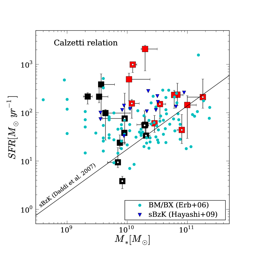
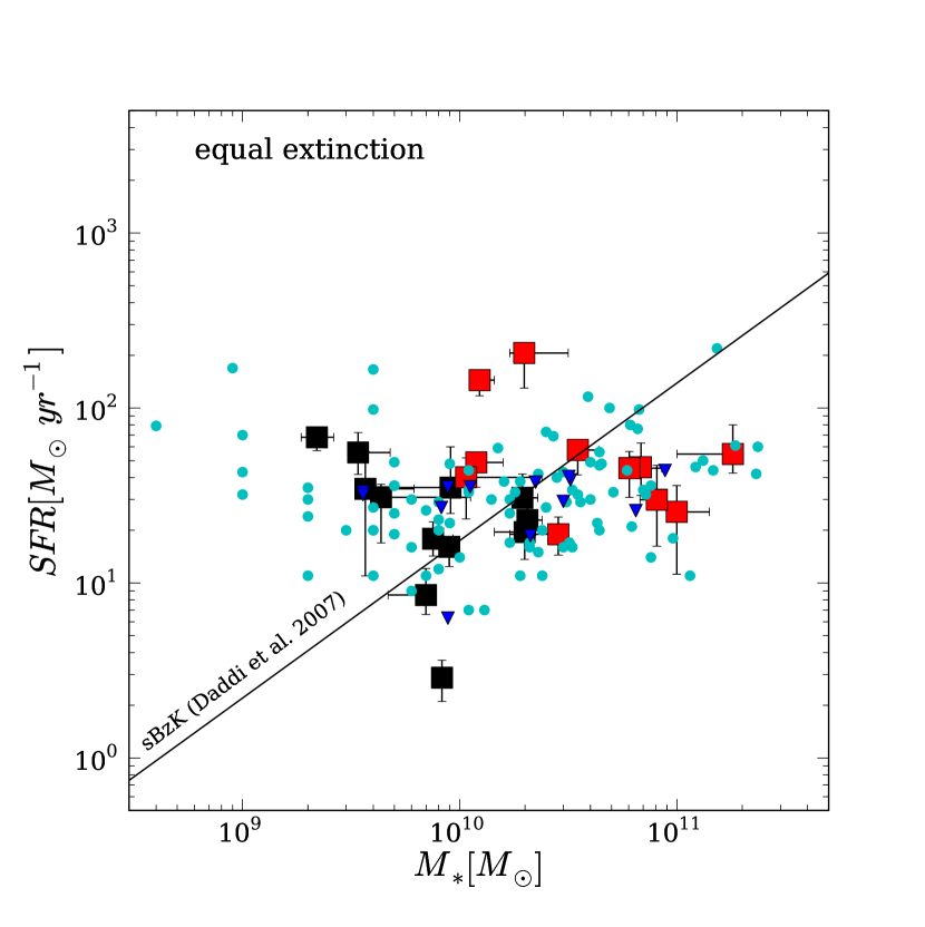
Figure 14.— Same as Figures 10, but plotted with the results from literature. The black solid line shows the correlation between SFR and stellar mass of sBzK galaxies (Daddi et al., 2007a). The results of Erb et al. (2006b) and Hayashi et al. (2009) are shown by cyan circles and blue triangles, respectively. White dots denote MIPS-excess galaxies.

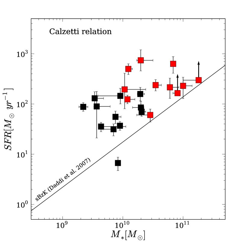
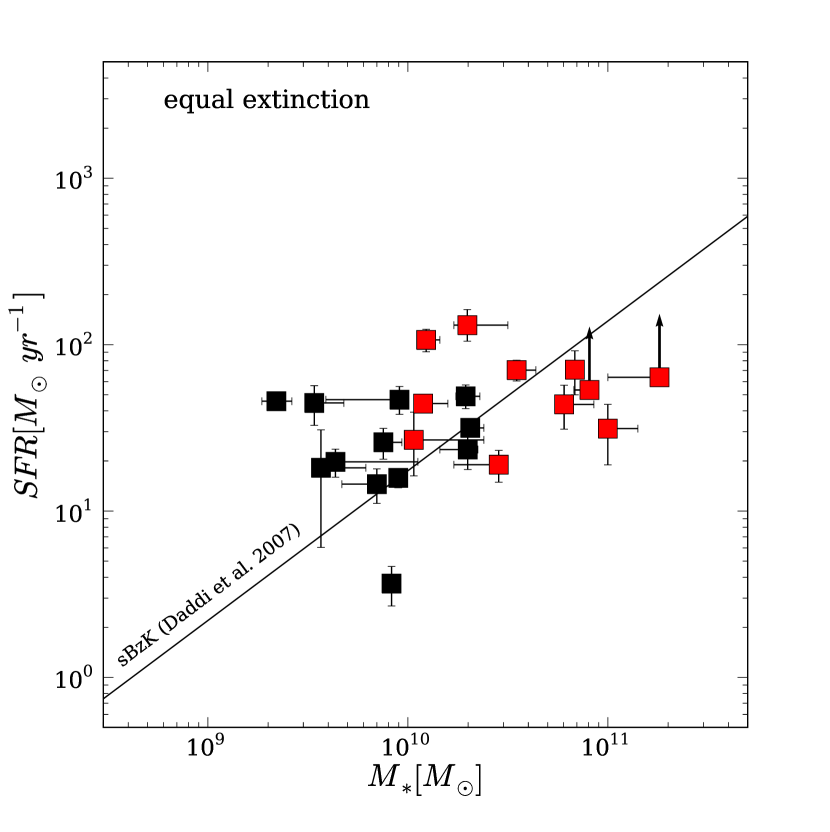
Figure 15.— Same as Figures 10, but the amout of extinction is estimated from $B-z$ color, as Daddi et al. (2007a).

Our result shows no correlation between stellar mass and SFR. However, Daddi et al. (2007a) demonstrated that BzK-selected star-forming galaxies have a tight correlation within 0.2 dex using SFR derived from UV and mid-IR. We compare our result for SFR and stellar mass with the Daddi et al. (2007a) relation (Figure 14). For the Calzetti (2001) relation, significant fractions of sBzK galaxies (4/18 and 4/19 for sBzK-MIPS and sBzK-non-MIPS, respectively) deviate from the correlation. Massive galaxies ($\gtrsim 10^{10}\,{\rm M}_{\odot}$) in our sample are distributed around the relation given by Daddi et al. (2007a), while some of the less massive galaxies ($\lesssim 10^{10}\,{\rm M}_{\odot}$) have much higher SFR than that expected from the correlation. Even for the equal-extinction case, which makes the SFRs of the higher SFR galaxies lower, there is still no correlation between stellar mass and SFR like that of Daddi et al. (2007a).

One of the reasons for the discrepancy could be the different extinction estimates used in Daddi et al. (2007a), who assumed a linear correlation between $B-z$ color and $E(B-V)$ derived from their SED fitting result (Daddi et al., 2004) to estimate extinction-corrected UV luminosities. In fact, if we apply the $E(B-V)$ values estimated from the $B-z$ color, the extinction corrected SFR(H$\alpha$) becomes smaller than the $E(B-V)$ values estimated from our stellar population analysis (Figure 15). Especially when the equal-extinction case is applied, the extinction corrected SFR(H$\alpha$)s are similar to the Daddi et al. (2007a) relation. Although our $E(B-V)$ values correlate with $B-z$ color, the correlation has larger scatter than that of Daddi et al. (2004) (Figure 16). The high-SSFR galaxies have larger $E(B-V)$ values than the galaxies with similar $B-z$ color.

The Daddi et al. (2007a) relation is also supported by Pannella et al. (2009), who shows the averaged properties of extinction from the radio-to-UV luminosity ratio using a large numbers ($\sim 12000$) of sBzK galaxies. They also find a strong correlation between the stellar mass and the amount of extinction, and thus the correlation accentuates the Daddi et al. (2007a) relation. In Figure 17, the amount of extinction of our galaxies is shown as a function of the stellar mass. Our results show a larger scatter than the errors of the correlation by Pannella et al. (2009). Although the extinction values of the low-SSFR galaxies correlate with the stellar masses, consistent with that of Pannella et al. (2009), the high-SSFR galaxies have higher extinctions than the low-SSFR galaxies with similar stellar masses. Because our emission line galaxies would be biased towards H$\alpha$ bright systems, galaxies that deviate from the average relation shown by Pannella et al. (2009) can be found, which probably results in the larger scatter.

Daddi et al. (2007a) also shows the same correlation using a SFR indicator unrelated to extinction. They estimated the SFR from the sum of the extinction uncorrected UV and mid-IR luminosities. On the other hand, Caputi et al. (2006a) reported that there exist significant fraction of lower mass ($\sim 10^{10}\,M_{\odot}$) galaxies with high SSFRs ($>10^{-8}\,{\rm yr}^{-1}$) at $z\sim 2$ using SFR inferred from the 24 $\mu$m flux. Daddi et al. (2007a) argues that the correlation is not accurately recovered with SFRs inferred only from mid-IR, due to a substantial presence of MIPS-excess galaxies, which are excluded from their sample. A MIPS-excess galaxy could harbor a heavily obscured AGN (Daddi et al., 2007b). However, our results on the SFR inferred from H$\alpha$ do not recover the correlation even if MIPS-excess galaxies are excluded from the sample. We calculate the MIPS excesses of our sample following Daddi et al. (2007a), and found that only a fraction of the high-SSFR galaxies show MIPS-excess. In Figure 14, MIPS-excess galaxies are denoted by white dots, which found to be more typically low-SSFR galaxies rather than high-SSFR galaxies.

Previous studies on the relation between SFR and stellar mass using the SFR derived from the H$\alpha$ luminosity show a similar trend to ours. The SFRs and stellar masses of BM/BX galaxies (Erb et al., 2006b) and sBzK galaxies (Hayashi et al., 2009) are also plotted on Figure 14. We convert the SFR and stellar mass of these studies to those calibrated with a Chabrier (2003) IMF. In the literature, they applied different extinction corrections to estimate the H$\alpha$ luminosities from that used to estimate the stellar extinction. The equal-extinction case is applied to the BM/BX galaxies, while the Calzetti (2001) relation to the sBzK galaxies. For comparison, we applied the same extinction correction to the samples in the literature as that for the present sample in each panel. There are no correlations between SFR and stellar mass of the samples in the both panels. However, some high-SSFR galaxies with SSFR$>10^{-8}\,{\rm yr}^{-1}$ appear when the Calzetti (2001) relation is applied.

In the studies for BM/BX and sBzK galaxies, validity of the extinction correction is confirmed with the consistency between SFR(H$\alpha$) and SFR(UV) (Erb et al., 2006b; Hayashi et al., 2009). We also confirmed the consistency between them in the previous section. The extinction corrected SFR(H$\alpha$) values assuming the equal-extinction case are consistent only for lower SFR galaxies (SFR$\lesssim 100\,{\rm M}_{\odot}\,{\rm yr}^{-1}$). SFRs calculated assuming the Calzetti (2001) relation are broadly consistent, but the SFR(H$\alpha$)s are systematically larger than the SFR(UV)s by 0.3 dex. These are almost consistent with the previous SFR(H$\alpha$) works. Although Erb et al. (2006b) applied only the equal-extinction case, galaxies with SFR(UV) $>100\,{\rm M}_{\odot}\,{\rm yr}^{-1}$ are rare in their sample. On the other hand, Hayashi et al. (2009), who used the Calzetti (2001) relation, also showed that their SFR(H$\alpha$) values are systematically larger than SFR(UV) by a factor of 3.

Recently, the relation between Balmer decrement and stellar continuum attenuation has been investigated for galaxies at low-to-medium redshift. Cowie & Barger (2008) studied spectroscopically confirmed $K$-selected sample at $0.05<z<0.475$. Their extinctions from the Balmer decrement and the continuum extinctions are equal on average. On the other hand, Moustakas & Kennicutt (2006) studied nearby galaxies, including starburst galaxies such as infrared-luminous galaxies. Comparison between their extinctions shows large scatter, but the average stellar-to-nebular extinction ratio is consistent with the Calzetti (2001) relation. The dust properties of the samples in these two studies are quite different. For example, the median reddening of Moustakas & Kennicutt (2006) sample is $E(B-V)\sim 0.24$, while about half of the galaxies of Cowie & Barger (2008) have $E(B-V)<0.01$. The values of reddening of the high-z samples discussed above and our samples are similar to that of Moustakas & Kennicutt (2006), but vary with the sample selection. The median values of reddening are $E(B-V)\sim 0.15,\,0.38$ for BM/BX galaxies by Erb et al. (2006b) and sBzK galaxies by Hayashi et al. (2009), respectively. This can imply that the Calzetti (2001) relation gives better estimation of the value of reddening for ionized gas in the active star-forming galaxies at high redshift.

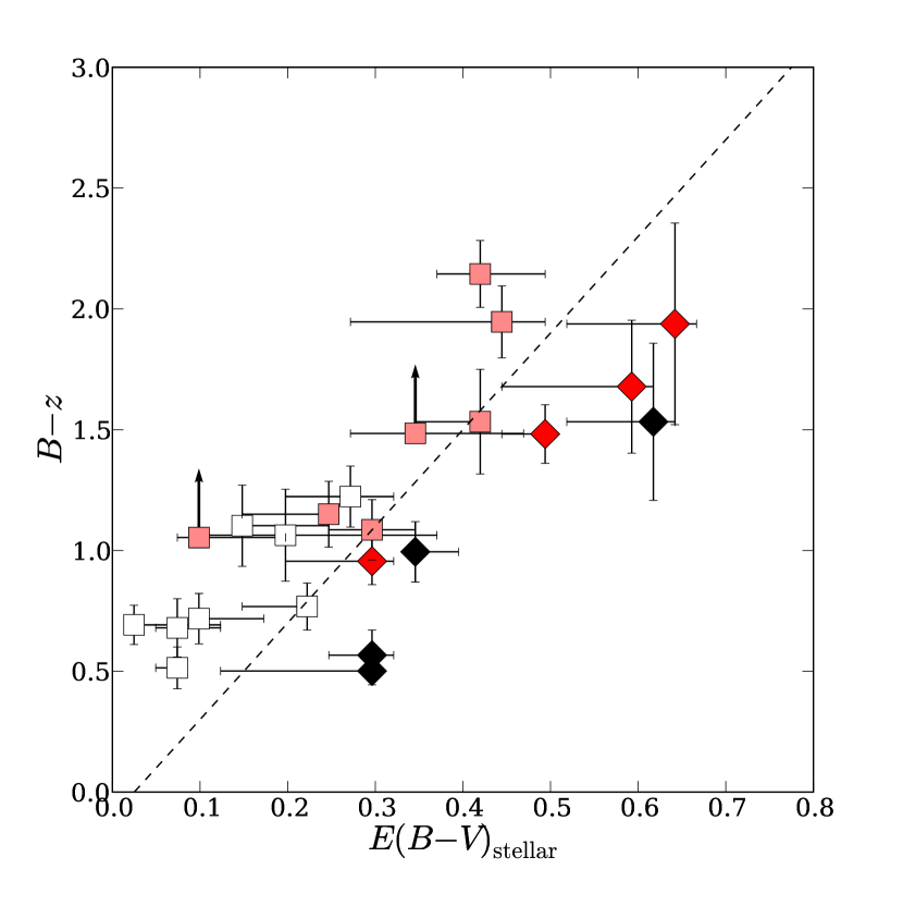
Figure 16.— Comparison of $E(B-V)$ with $B-z$ color for the present sample. Symbols are same as in Figure 12. The Dashed line shows the linear correlation between $B-z$ color and $E(B-V)$ by Daddi et al. (2004).

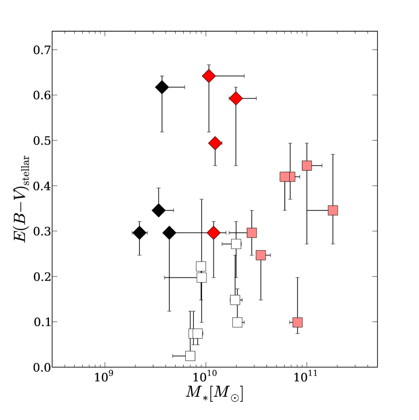
Figure 17.— Comparison of stellar mass with $E(B-V)$ for the present sample. Symbols are same as in Figure 12.

5.2. Metallicity

The gas-phase metallicity reflects the past star-formation history of a galaxy since the heavy elements are produced by nuclear fusion in stars and fed back into gas. Therefore, it is expected that the gas-phase metallicity of galaxies in the high-z universe is lower than that in the local Universe. The metallicities were found to be lower in high-z galaxies than those in local galaxies (e.g., Shapley et al., 2004; Savaglio et al., 2005; Erb et al., 2006a; Maiolino et al., 2008; Hayashi et al., 2009; Pérez-Montero et al., 2009; Lamareille et al., 2009). We measured the gas-phase metallicity of our samples to investigate their star-formation histories.

The gas-phase metallicity is estimated from the [N ii]$\lambda$6583-H$\alpha$ line ratio (N2 index), defined by

$$N2\equiv\log{\{[\mathrm{N_{II}}]\lambda 6583/\mathrm{H\alpha}\}},$$ (9)

which correlates with oxygen abundance (Storchi-Bergmann et al., 1994). The relation between the N2 index and gas-phase oxygen abundance is given by

$$12+\log{(\mathrm{O/H})}=8.90+0.57\times N2$$ (10)

(Pettini & Pagel, 2004). [N ii] and H$\alpha$ are so close to each other in wavelength that the ratio is not affected by reddening. Therefore, the N2 index has been used to estimate the oxygen abundances of distant galaxies (e.g., Shapley et al., 2004; Erb et al., 2006a; Hayashi et al., 2009). We note that the N2 index saturates at $\sim 1\,{\rm Z}_{\odot}$ ($12+\log(\rm O/H)=8.66;$ Asplund et al., 2004).

In order to gain a sufficiently high S/N to reliably measure the line flux ratio, we stacked the [N ii]-H$\alpha$ emission lines. We divided the present sample into three groups based on stellar masses at $9\times 10^{9}\,{\rm M}_{\odot}$ and $2.5\times 10^{10}\,{\rm M}_{\odot}$. In addition, we also divide the sample into two groups based on a SSFR of $10^{-8}\,{\rm yr}^{-1}$. The stacking, measurement of flux, and estimates of error are performed in the same manner as described in §3.3. The results are plotted in Figure 18 as a function of the median stellar mass of each group. For comparison, $\sim 39500$ local objects from SDSS DR4, local Lyman Break Analog (LBA) galaxies (Overzier et al., 2010), BM/BX galaxies (Erb et al., 2006a), and sBzK galaxies (Hayashi et al., 2009) are also plotted with the same calibration.

The mass-metallicity properties of our high-SSFR galaxies are possibly different from that of rest-UV selected galaxies. The mass-metallicity relation of the two largest mass bins is consistent with that of BM/BX galaxies described by Erb et al. (2006a), while the smallest mass bin has higher metallicity than the similar mass bins of Erb et al. (2006a); our sample is closer to the local galaxies. The discrepancy in the smallest mass bin could be due to the galaxies with high SSFR. The high-SSFR group has higher metallicity, close to that of the local galaxies with similar stellar mass. As shown in Figure 10, high-SSFR galaxies dominate our sample in the smallest mass bin, while most of the galaxies in Erb et al. (2006a) have SSFR smaller than $10^{-8}\,{\rm yr}^{-1}$.

The $K$-band selected samples would provide many galaxies with high SSFR and metallicity. The existence of higher metallicity galaxies in $K$-selected sample is also supported by the observations of sBzK galaxies by Hayashi et al. (2009), as shown in Figure 18. On the other hand, the local LBAs, which are local analogs of high-z UV-selected galaxies, tend to have a lower mass-metallicity relation. This would suggest that the sample by Erb et al. (2006a) is biased toward lower metallicities due to the rest-UV selection. The results indicate that in order to reveal the unbiased cosmic evolution of mass-metallicity relation, we need to evaluate metallicities of a larger sample of $K$-band selected (i.e., mass-selected) galaxies.

It is surprising that the high-SSFR galaxies have already acquired metallicities as high as local galaxies at $z\sim 2$. The age of the stellar population of the high-SSFR galaxies is young, so that the metal enrichment must have occurred in a short timescale. The N2 index is known to be sensitive to a hard ionizing radiation field from an AGN or strong shock excitation and ionization parameter (Kewley & Dopita, 2002). In fact, our stacked [O iii]$\lambda$5007/H$\beta$ and [N ii]$\lambda$6583/H$\alpha$ line ratios show evidence for a harder ionizing spectrum. If the metallicity is really high, the result is in conflict with the observations of local galaxies. These galaxies can not keep their stellar masses and metallicities after the observed epoch, because the studies for local galaxies demonstrate that galaxies in a similar mass range formed a significant fraction of their stars in the low redshift universe (Heavens et al., 2004), suggesting that these local galaxies must have increased their metallicity recently. It is possible that such high-SSFR galaxies evolved into larger stellar mass galaxies with low star-forming efficiency in the local universe, depleting the gas and/or merging with higher mass galaxies.

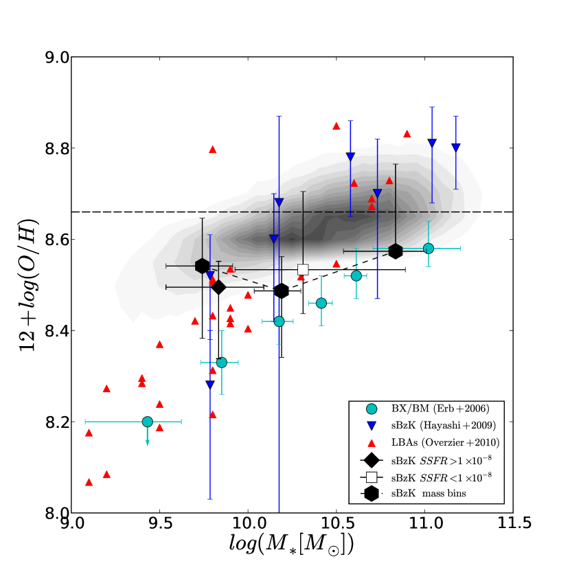
Figure 18.— Oxygen abundance derived from the N2 index for the stacked [N ii]-H$\alpha$ spectra, which are grouped by (1) stellar mass at $9\times 10^{9}\,M_{\odot}$ and $2.5\times 10^{10}\,M_{\odot}$ (black hexagons) and (2) SSFR at $10^{-8}\,{\rm yr}^{-1}$ (black diamond and open square), as a function of the median stellar mass of each group. Horizontal error bars indicate the 64% quantiles of stellar masses in the respective bins, while vertical bars indicate the error of the N2 index measurements derived from bootstrap sampling. The results of the stacked spectra of BM/BX galaxies by Erb et al. (2006a) are plotted with cyan circles. The sBzK galaxies by Hayashi et al. (2009) and the local Lyman Break Analog (LBA) galaxies by Overzier et al. (2010) are plotted with blue downward triangles and red upward triangles, respectively. Gray contours show the plots of $\sim 395000$ objects from SDSS DR4 with the same calibration of oxygen abundance. The horizontal dashed line shows solar metallicity ($12+\log(\rm O/H)=8.66;$ Asplund et al., 2004), where the N2 index calibration saturates.

5.3. Contribution to the Cosmic SFR Density

We estimate the contribution of the observed galaxies to the cosmic SFR density at $z\sim 2$ with the SFR(H$\alpha$)s, dividing the sample into two groups with SSFR $>10^{-8}\,{\rm yr}^{-1}$ and $<10^{-8}\,{\rm yr}^{-1}$ for the extinction corrected SFRs with the Calzetti (2001) relation. Since we observed only a limited number of sBzK galaxies, we need to assume that the SFR and redshift distributions of the other galaxies are the same as the observed galaxies; this is not unreasonable since we randomly selected the present sample from the sBzK-MIPS and sBzK-non-MIPS population. First, we further divide the sample based on the MIPS detection in the public catalog. Second, we calculated the total SFR in a certain group; we multiply the total SFR in the group by the ratio of the number of the entire galaxies in the group to that of the number of galaxies observed. In the calculation of total SFR, we assumed that the SFR of the galaxies without H$\alpha$ detection is negligible; we set those SFRs to zero. Then the total SFRs of galaxies with and without MIPS detection are summed. Third, we divide the total SFR by the expected detection rate of H$\alpha$ emission line (87.7%; see §4.1) to recover the H$\alpha$ emission lines not detected due to strong sky emission lines or atmospheric absorption bands. Finally, we divide the total SFRs by comoving volume of the survey region for $1.4<z<2.5$.

The resultant total cosmic SFR densities of the sBzK galaxies are $0.136^{+0.020}_{-0.028}$, $0.029^{+0.002}_{-0.002}$  ${\rm M}_{\odot}\,{\rm yr}^{-1}\,{\rm Mpc}^{-3}$ for extinction correction calculated using the Calzetti (2001) relation and the equal-extinction case, respectively. As we see in the previous discussions, the relation between extinction estimated from the stellar continuum and the emission lines probably depend on the intrinsic luminosities, and thus the SFRs. To examine this effect, when we apply extinction correction with the Calzetti (2001) relation for the sBzK-MIPS galaxies and equal extinction for the sBzK-non-MIPS galaxies (differential correction), the result is $0.089^{+0.008}_{-0.021}$. In any case of the extinction correction, high-SSFR galaxies have a large contribution to the SFR density. Although these galaxies account for only $\sim 20\,\%$ of all of the galaxies, they contribute to $\sim 75\,\%$ of the SFR density for the extinction correction with the Calzetti (2001) relation and the differential extinction. Even for the equal-extinction case, they contribute to no less than $\sim 50\,\%$ of the SFR density.

We compare our SFR density at $z\sim 2$ with previous works (e.g., Hopkins, 2004; Hopkins & Beacom, 2006 and the references therein; Wang et al., 2006; Caputi et al., 2007). If we use the same calibration of IMF as that of these studies, the SFR densities are 0.203, 0.044, 0.134 ${\rm M}_{\odot}\,{\rm yr}^{-1}\,{\rm Mpc}^{-3}$ for the Calzetti (2001) relation, the equal-extinction case, and the differential correction, respectively. The values compiled by Hopkins (2004) and Hopkins & Beacom (2006) are 0.05-0.38 ${\rm M}_{\odot}\,{\rm yr}^{-1}\,{\rm Mpc}^{-3}$, which are consistent with both of those with the Calzetti (2001) relation and differential extinction. Recent studies on the SFR density at $z\sim 2$ using IR luminosities (850 $\mu$m; Wang et al., 2006; 24 $\mu$m; Caputi et al., 2007) show slightly lower SFR densities (0.08-0.09 ${\rm M}_{\odot}\,{\rm yr}^{-1}\,{\rm Mpc}^{-3}$), which are still consistent with the differential extinction correction. This would also suggest that the relation between the dust properties of the stellar continuum and the emission lines are different depending on the intrinsic SFR. The SFR density using the equal-extinction case is lower than that of any study. The lower SFR density implies that applying the equal-extinction case to all galaxies underestimates SFR(H$\alpha$).

6. Summary and Conclusions

We performed near-infrared spectroscopic observations for 37 $BzK$ color selected star-forming galaxies with MOIRCS on the Subaru Telescope. The sample galaxies are picked from the deep $K_{s}$-selected catalog of MODS. We select 18 of our sample from the publicly available 24 $\mu$m source catalog of MIPS on board the $Spitzer$ Space Telescope. In order to avoid contamination by AGNs, we exclude the BzKs detected in the Chandra Deep Field-North 2 Ms Point-Source Catalogs. All of the sample galaxies have strong 1.6 $\mu$m bumps in their SEDs, so that their optical emission is thought to be dominated by the stellar continuum. The H$\alpha$ emission lines are detected from 23 galaxies, of which the median redshift is $z=2.12$. In the diagnostic diagram with [O iii]$\lambda$5007/H$\beta$ and [N ii]$\lambda$6583/H$\alpha$, the line ratios of the stacked spectra are above that found for local star-forming galaxies but closer to the expectations from star-formation activity rather than AGN activity.

We derived the SFRs from the extinction-corrected H$\alpha$ luminosities. The extinction correction for the H$\alpha$ luminosity is estimated from the SED fitting of multi-band photometric data with stellar population models of exponentially declining SFR and the Calzetti et al. (2000) extinction curve. To estimate the extinction correction for the ionized gas, we assumed the Calzetti (2001) relation ($E(B-V)_{\rm stellar}=0.44\times E(B-V)_{\rm gas}$) as well as the equal-extinction case $E(B-V)_{\rm stellar}=E(B-V)_{\rm gas}$, and compared the extinction corrected SFRs. Although the Balmer decrement of the stacked emission lines is consistent with the Calzetti (2001) relation, a fraction of the H$\beta$ detected galaxies are consistent with the equal-extinction case. We further investigated these galaxies by comparing the extinction corrected H$\alpha$ luminosities with other SFR indicators. The comparison with the UV and MIPS 24 $\mu$m flux shows that the SFRs of lower SFR galaxies ($\lesssim 100\,{\rm M}_{\odot}\,{\rm yr}^{-1}$) are in good agreement for the equal-extinction case, while those of the higher SFR galaxies agree for the Calzetti (2001) relation. This implies that the relation between the dust properties of the stellar continuum and emission lines are different depending on the intrinsic SFR (differential extinction correction). If the Calzetti relation is assumed, a fraction of the high-SFR galaxies should be detected in radio, (sub-)mm, and X-ray catalogs, but none of them except one AzTEC source are detected. We could not explain the reason for this discrepancy consistently. However, most of the discrepancy could be explained by the short timescale of star-formation activity, because the younger ages of the stellar population are derived from our SED analysis. We note that other mechanisms (e.g., top-heavy IMF, lower dust temperature, etc.) could also explain a part of the discrepancy.

We compared the extinction-corrected H$\alpha$ luminosities with the stellar masses obtained from the SED fitting. When we apply the Calzetti (2001) relation, the comparison shows no correlation between SFR and stellar mass. A fraction of the galaxies with stellar mass smaller than $\sim 10^{10}\,{\rm M}_{\odot}$ show SFRs higher than $\sim 100\,{\rm M}_{\odot}\,{\rm yr}^{-1}$. The SSFRs of these galaxies are higher than $\sim 10^{-8}\,{\rm yr}^{-1}$. Even if equal extinction is applied, their SSFRs are still high (${\rm SSFR}>3.5\times 10^{-9}\,{\rm yr}^{-1}$). This is inconsistent with the correlation demonstrated by Daddi et al. (2007a). Our value of extinction correction shows large scatter against $B-z$ color and stellar mass, with which Daddi et al. (2004) and Pannella et al. (2009) show strong correlations. From the best-fit parameters of the SED fitting for these high-SSFR galaxies, we found that the average age of the stellar population is younger than 100 Myr, which are consistent with SFR age (${\rm SSFR}^{-1}$) with the Calzetti (2001) relation. We also calculate the contribution of the present H$\alpha$ emission to the cosmic SFR density at $z\sim 2$. Our results are consistent with previous works, if we apply the Calzetti (2001) relation or differential extinction correction. The high-SSFR galaxies significantly contribute ($50-75\%$) to the cosmic SFR density.

The metallicity of the high-SSFR galaxies, which is estimated from the N2 index, is larger than that expected from the mass-metallicity relation of UV-selected galaxies at $z\sim 2$ by Erb et al. (2006a). Although metallicities estimated from the N2 index is known to have significant uncertainties due to the harder ionizing radiation field and ionization parameter, the high metallicity comparable to galaxies in the same mass range is inconsistent with the known star-formation history of such galaxies in the local universe, which formed a significant fraction of their stars in the low redshift universe. The high-SSFR galaxies, therefore, possibly evolve into larger stellar mass galaxies with low star-forming efficiency, depleting the gas.

References

- Adelman-McCarthy et al. (2008) Adelman-McCarthy, J. K., et al. 2008, ApJS, 175, 297
- Alexander et al. (2002) Alexander, D. M., Aussel, H., Bauer, F. E., Brandt, W. N., Hornschemeier, A. E., Vignali, C., Garmire, G. P., & Schneider, D. P. 2002, ApJ, 568, L85
- Alexander et al. (2003) Alexander, D. M., et al. 2003, AJ, 126, 539
- Asplund et al. (2004) Asplund, M., Grevesse, N., Sauval, A. J., Allende Prieto, C., & Kiselman, D. 2004, A&A, 417, 751
- Baldwin et al. (1981) Baldwin, J. A., Phillips, M. M., & Terlevich, R. 1981, PASP, 93, 5
- Barger et al. (2008) Barger, A. J., Cowie, L. L., & Wang, W.-H. 2008, ApJ, 689, 687
- Biggs & Ivison (2006) Biggs, A. D., & Ivison, R. J. 2006, MNRAS, 371, 963
- Bolzonella et al. (2000) Bolzonella, M., Miralles, J.-M., & Pelló, R. 2000, A&A, 363, 476
- Bruzual & Charlot (2003) Bruzual, G., & Charlot, S. 2003, MNRAS, 344, 1000
- Calzetti (2001) Calzetti, D. 2001, PASP, 113, 1449
- Calzetti et al. (2000) Calzetti, D., Armus, L., Bohlin, R. C., Kinney, A. L., Koornneef, J., & Storchi-Bergmann, T. 2000, ApJ, 533, 682
- Capak et al. (2004) Capak, P., et al. 2004, AJ, 127, 180
- Caputi et al. (2006a) Caputi, K. I., et al. 2006a, ApJ, 637, 727
- Caputi et al. (2006b) Caputi, K. I., Dole, H., Lagache, G., McLure, R. J., Dunlop, J. S., Puget, J.-L., Le Floc’h, E., & Pérez-González, P. G. 2006b, A&A, 454, 143
- Caputi et al. (2007) Caputi, K. I., et al. 2007, ApJ, 660, 97
- Castelli & Kurucz (2004) Castelli, F., & Kurucz, R. L. 2004, arXiv:astro-ph/0405087
- Chabrier (2003) Chabrier, G. 2003, PASP, 115, 763
- Chapin et al. (2009) Chapin, E. L., et al. 2009, MNRAS, 398, 1793
- Chapman et al. (2005) Chapman, S. C., Blain, A. W., Smail, I., & Ivison, R. J. 2005, ApJ, 622, 772
- Chary & Elbaz (2001) Chary, R., & Elbaz, D. 2001, ApJ, 556, 562
- Cohen (2001) Cohen, J. G. 2001, AJ, 121, 2895
- Cohen et al. (2000) Cohen, J. G., Hogg, D. W., Blandford, R., Cowie, L. L., Hu, E., Songaila, A., Shopbell, P., & Richberg, K. 2000, ApJ, 538, 29
- Condon (1992) Condon, J. J. 1992, ARA&A, 30, 575
- Cowie & Barger (2008) Cowie, L. L., & Barger, A. J. 2008, ApJ, 686, 72
- Cowie et al. (2004) Cowie, L. L., Barger, A. J., Hu, E. M., Capak, P., & Songaila, A. 2004, AJ, 127, 3137
- Daddi et al. (2004) Daddi, E., Cimatti, A., Renzini, A., Fontana, A., Mignoli, M., Pozzetti, L., Tozzi, P., & Zamorani, G. 2004, ApJ, 617, 746
- Daddi et al. (2007a) Daddi, E., et al. 2007a, ApJ, 670, 156
- Daddi et al. (2007b) Daddi, E., et al. 2007b, ApJ, 670, 173
- Dahlen et al. (2007) Dahlen, T., Mobasher, B., Dickinson, M., Ferguson, H. C., Giavalisco, M., Kretchmer, C., & Ravindranath, S. 2007, ApJ, 654, 172
- Davé (2008) Davé, R. 2008, MNRAS, 385, 147
- Dawson et al. (2001) Dawson, S., Stern, D., Bunker, A. J., Spinrad, H., & Dey, A. 2001, AJ, 122, 598
- Denicoló et al. (2002) Denicoló, G., Terlevich, R., & Terlevich, E. 2002, MNRAS, 330, 69
- Erb et al. (2006a) Erb, D. K., Shapley, A. E., Pettini, M., Steidel, C. C., Reddy, N. A., & Adelberger, K. L. 2006a, ApJ, 644, 813
- Erb et al. (2003) Erb, D. K., Shapley, A. E., Steidel, C. C., Pettini, M., Adelberger, K. L., Hunt, M. P., Moorwood, A. F. M., & Cuby, J.-G. 2003, ApJ, 591, 101
- Erb et al. (2006b) Erb, D. K., Steidel, C. C., Shapley, A. E., Pettini, M., Reddy, N. A., & Adelberger, K. L. 2006b, ApJ, 647, 128
- Förster Schreiber et al. (2009) Förster Schreiber, N. M., et al. 2009, ApJ, 706, 1364
- Giavalisco et al. (2004) Giavalisco, M., et al. 2004, ApJ, 600, L93
- Grazian et al. (2007) Grazian, A., et al. 2007, A&A, 465, 393
- Greve et al. (2008) Greve, T. R., Pope, A., Scott, D., Ivison, R. J., Borys, C., Conselice, C. J., & Bertoldi, F. 2008, MNRAS, 389, 1489
- Grimm et al. (2003) Grimm, H.-J., Gilfanov, M., & Sunyaev, R. 2003, MNRAS, 339, 793
- Hayashi et al. (2009) Hayashi, M., et al. 2009, ApJ, 691, 140
- Heavens et al. (2004) Heavens, A., Panter, B., Jimenez, R., & Dunlop, J. 2004, Nature, 428, 625
- Holland et al. (1999) Holland, W. S., et al. 1999, MNRAS, 303, 659
- Hopkins (2004) Hopkins, A. M. 2004, ApJ, 615, 209
- Hopkins & Beacom (2006) Hopkins, A. M., & Beacom, J. F. 2006, ApJ, 651, 142
- Iye et al. (2004) Iye, M., et al. 2004, PASJ, 56, 381
- Kajisawa et al. (2009) Kajisawa, M., et al. 2009, ApJ, 702, 1393
- Kauffmann et al. (2003) Kauffmann, G., et al. 2003, MNRAS, 346, 1055
- Kennicutt (1998) Kennicutt, R. C., Jr. 1998, ARA&A, 36, 189
- Kewley et al. (2001) Kewley, L. J., Dopita, M. A., Sutherland, R. S., Heisler, C. A., & Trevena, J. 2001, ApJ, 556, 121
- Kewley & Dopita (2002) Kewley, L. J., & Dopita, M. A. 2002, ApJS, 142, 35
- Kreysa et al. (1998) Kreysa, E., et al. 1998, Proc. SPIE, 3357, 319
- Kriek et al. (2006) Kriek, M., et al. 2006, ApJ, 645, 44
- Kriek et al. (2007) Kriek, M., et al. 2007, ApJ, 669, 776
- Kriss (1994) Kriss, G. 1994, Astronomical Data Analysis Software and Systems, 3, 437
- Lamareille et al. (2009) Lamareille, F., et al. 2009, A&A, 495, 53
- Maiolino et al. (2008) Maiolino, R., et al. 2008, A&A, 488, 463
- Maraston (2005) Maraston, C. 2005, MNRAS, 362, 799
- Moustakas & Kennicutt (2006) Moustakas, J., & Kennicutt, R. C., Jr. 2006, ApJS, 164, 81
- Osterbrock (1989) Osterbrock, D. E. 1989, Research supported by the University of California, John Simon Guggenheim Memorial Foundation, University of Minnesota, et al. Mill Valley, CA, University Science Books, 1989, 422 p.,
- Overzier et al. (2010) Overzier, R. A., Heckman, T. M., Schiminovich, D., Basu-Zych, A., Gonçalves, T., Martin, D. C., & Rich, R. M. 2010, ApJ, 710, 979
- Pannella et al. (2009) Pannella, M., et al. 2009, ApJ, 698, L116
- Papovich et al. (2007) Papovich, C., et al. 2007, ApJ, 668, 45
- Pérez-González et al. (2005) Pérez-González, P. G., et al. 2005, ApJ, 630, 82
- Pérez-González et al. (2008) Pérez-González, P. G., et al. 2008, ApJ, 675, 234
- Pérez-Montero et al. (2009) Pérez-Montero, E., et al. 2009, A&A, 495, 73
- Peeters et al. (2004) Peeters, E., Spoon, H. W. W., & Tielens, A. G. G. M. 2004, ApJ, 613, 986
- Perera et al. (2008) Perera, T. A., et al. 2008, MNRAS, 391, 1227
- Pettini & Pagel (2004) Pettini, M., & Pagel, B. E. J. 2004, MNRAS, 348, L59
- Pope et al. (2005) Pope, A., Borys, C., Scott, D., Conselice, C., Dickinson, M., & Mobasher, B. 2005, MNRAS, 358, 149
- Pope et al. (2006) Pope, A., et al. 2006, MNRAS, 370, 1185
- Raimann et al. (2000) Raimann, D., Storchi-Bergmann, T., Bica, E., Melnick, J., & Schmitt, H. 2000, MNRAS, 316, 559
- Ranalli et al. (2003) Ranalli, P., Comastri, A., & Setti, G. 2003, A&A, 399, 39
- Reddy et al. (2006a) Reddy, N. A., Steidel, C. C., Fadda, D., Yan, L., Pettini, M., Shapley, A. E., Erb, D. K., & Adelberger, K. L. 2006a, ApJ, 644, 792
- Reddy et al. (2006b) Reddy, N. A., Steidel, C. C., Erb, D. K., Shapley, A. E., & Pettini, M. 2006b, ApJ, 653, 1004
- Rousselot et al. (2000) Rousselot, P., Lidman, C., Cuby, J.-G., Moreels, G., & Monnet, G. 2000, A&A, 354, 1134
- Salpeter (1955) Salpeter, E. E. 1955, ApJ, 121, 161
- Savaglio et al. (2005) Savaglio, S., et al. 2005, ApJ, 635, 260
- Sawicki (2002) Sawicki, M. 2002, AJ, 124, 3050
- Shapley et al. (2004) Shapley, A. E., Erb, D. K., Pettini, M., Steidel, C. C., & Adelberger, K. L. 2004, ApJ, 612, 108
- Skrutskie et al. (2006) Skrutskie, M. F., et al. 2006, AJ, 131, 1163
- Smartt et al. (2009) Smartt, S. J., Eldridge, J. J., Crockett, R. M., & Maund, J. R. 2009, MNRAS, 395, 1409
- Stetson (1992) Stetson, P. B. 1992, Astronomical Data Analysis Software and Systems I, 25, 297
- Storchi-Bergmann et al. (1994) Storchi-Bergmann, T., Calzetti, D., & Kinney, A. L. 1994, ApJ, 429, 572
- Suzuki et al. (2008) Suzuki, R., et al. 2008, PASJ, 60, 1347
- Swinbank et al. (2006) Swinbank, A. M., Chapman, S. C., Smail, I., Lindner, C., Borys, C., Blain, A. W., Ivison, R. J., & Lewis, G. F. 2006, MNRAS, 371, 465
- Swinbank et al. (2005) Swinbank, A. M., et al. 2005, MNRAS, 359, 401
- Tokoku (2007) Tokoku C. 2007, PhD thesis, Tohoku University
- Treu et al. (2005) Treu, T., Ellis, R. S., Liao, T. X., & van Dokkum, P. G. 2005, ApJ, 622, L5
- Veilleux & Osterbrock (1987) Veilleux, S., & Osterbrock, D. E. 1987, ApJS, 63, 295
- Wang et al. (2006) Wang, W.-H., Cowie, L. L., & Barger, A. J. 2006, ApJ, 647, 74
- Wilson et al. (2008) Wilson, G. W., et al. 2008, MNRAS, 386, 807
- Wirth et al. (2004) Wirth, G. D., et al. 2004, AJ, 127, 3121
- Yun et al. (2001) Yun, M. S., Reddy, N. A., & Condon, J. J. 2001, ApJ, 554, 803